A Memristor-Based Colpitts Oscillator Circuit

Abstract

This paper investigates a simple memristor emulator consisting of a diode bridge and a capacitor. It exhibits pinched hysteresis loops, and what is more striking is the higher frequency, as it operates up to greater than 5 MHz. Based on the proposed memristor, a higher-frequency Colpitts circuit was established. According to the mathematical model of the system, the system only possesses one unstable equilibrium point. Period doubling bifurcation, reverse periodic doubling bifurcation, different types of periodic and chaotic orbits, transient chaos, coexisting bifurcations and offset boosting are depicted. More interestingly, it has coexisting multiple attractors with different topologies, such as a chaotic attractor accompanied with periodic orbits, period-1 orbits with bicuspid structure and periodic-2 orbits with tridentate structure. Moreover, a hardware circuit using discrete components was fabricated and experimental measurements were consistent with the MATLAB numerical results, further confirming the real feasibility of the proposed circuit.

1. Introduction

A memristor is a two-terminal device that offers a constitutive relation of flux and charge [1]. Since the successful implementation of a memristor in TiO₂ in HP Lab in 2008 [2], its promising application in logic gates [3,4], non-volatile memory [5,6], neuromorphic computing and neurons [7,8,9,10,11,12], signal processing [13,14] and nonlinear systems [15,16,17] has attracted extensive attention. Despite commercial chips having been fabricated [18], to date, the availability of memristors as mainstream electronic components remains limited because of their fabrication complexity and high cost. In order to study the dynamics of nonlinear circuits and systems containing memristors, various kinds of memristor emulators have been reported to simulate the basic characteristics of memristors.

So far we know, memristor emulators generally use kinds of electronic components such as MOSFET [19,20,21], diode bridge [22,23,24,25,26,27,28,29,30,31,32], various analog building blocks such as operational amplifiers and multipliers [33,34], differential difference current conveyors (DDCCs) [35], second generation current conveyors (CCIIs) [36], current conveyor transconductance amplifier (CCTAs) [37], voltage difference transconductance amplifiers (VDTAs) [38], differential voltage current conveyor (DVCCs) [39] and so on.

Corinto F. put forward a memristor emulator combined with a passive diode bridge and second-order RLC filter in 2012 [22]. Subsequently, improved memristive symmetric diode bridge emulators [23,24,25,26,27,28,29] and asymmetric diode bridges [30,31,32] were reported, and they show symmetrical or asymmetrical pinched hysteresis loops in the voltage–current domain. Abundant chaotic circuit based on memristive diode bridge emulators have been proposed, and can display some complex and interesting nonlinear phenomena such as coexisting attractors [27,29,30,31,32], bursting [28,30] and hyperchaos [32], just to name a few.

Memristors for high-frequency applications are also an area of research. In 2014, a DDCC-based ground memristor that operates up to 1 MHz frequency was designed [35]. In 2017, Ranjan proposed a simpler memristor simulator mainly consisting of one CCII and one multiplier, where DC voltages and adjustable resistors were used to ensure zero crossing of the pinched hysteresis loop, and its highest frequency could reach 860 kHz [36]. In the same year, Ranjan used a current transmission transconductance amplifier (CCTA) to realize the transformation of grounding, floating, incremental model or decrement models quickly without changing the circuit structure; however, the operating frequencies of the memristor emulator circuit on printed circuit board were in the range of few hundreds of kHz only because of limitations on the bandwidth and slew rate of BJT based ICs [37]. In 2018, a grounded memristor emulator circuit consisting of seven MOS transistors and one grounded capacitor was presented, and the maximum allowable frequency reached 50 MHz [19]. In 2019, only three MOS tubes and a capacitor were used to realize a floating memristor with a maximum frequency of 13 MHz [20]. In 2021, Vista proposed a floating memristor based on single VDTA that has the maximum allowable frequency (50 MHz) [38]. In 2022, Anamika used VDTA and OTA to realize a dual-mode grounded memristor emulator with 1 MHz operating frequency [39]. A floating memristor emulator (the maximum frequency was 50 MHz) based on four MOSFETs only was developed [21]. The above literature addresses memristor emulators that operate up to higher frequencies.

A summary of the existing works on memristor emulators with higher frequency are illustrated in

Table 1. Comparative analysis of the proposed work on memristor emulators with higher frequencies.

Ref.	Essential Components	Power Supply	Floating/ Grounded	Operating Frequency
[19]	7 MOSFETs	±0.9 V DC voltages	Grounded	50 MHz
[20]	3 MOSFETs	10 μA	Floating	13 MHz
[21]	4 MOSFETs	No	Floating	50 MHz
[35]	DDCC	±1.5 V DC	Grounded	1 MHz
[36]	1 CCII, 1 multiplier	±10 V DC	Grounded	860 kHz
[37]	CCTA	±1.5 V DC	Floating/ grounded	hundreds of kHz
[38]	VDTA	±0.9 V DC	Floating	50 MHz
[39]	VDTA, OTA	±0.9 V DC, ±1.2 V DC	Grounded	1 MHz
Proposed work	Diode bridge	No	Floating	5 MHz

. They mainly center on MOSFET [19,20,21] or analog building blocks [35,36,37,38,39]. Except for [21], the memristive emulators all need power supply. A memristive diode bridge emulator containing only passive devices is known with simple circuit structure, without ground limitation. The existing works on diode bridge memristor emulator circuits [22,23,24,25,26,27,28,29,30,31,32] have not covered the higher frequency characteristics. So far as we know, it is necessary to be concerned about the higher frequency characteristics of diode bridge memristive emulators.

This paper proposes a floating memristor emulator configuration based on diode bridges, and it comprises one diode bridge and one capacitor. The numerical and circuit simulation results suggest that the proposed memristor emulator works at more than 5 MHz operating frequency. By introducing the proposed memristor into a Colpitts chaotic oscillator circuit, the circuit can generate coexisting multiple attractors.

The remaining sections of this paper are organized as follows. In Section 2, a floating memristor emulator based on diode bridges is addressed, and has a pinched hysteresis loop. In Section 3, a memristive-based Colpitts circuit and its mathematical model, equilibrium and stability are depicted. In Section 4, numerical simulations of the proposed circuit are performed by using basins of attraction, phase portraits, bifurcation diagrams and Lyapunov exponents and so on. The system can produce coexisting attractors. In Section 5, hardware experiments on a breadboard are performed, and the results are according with numerical simulations. Lastly, the conclusions are summarized in Section 6.

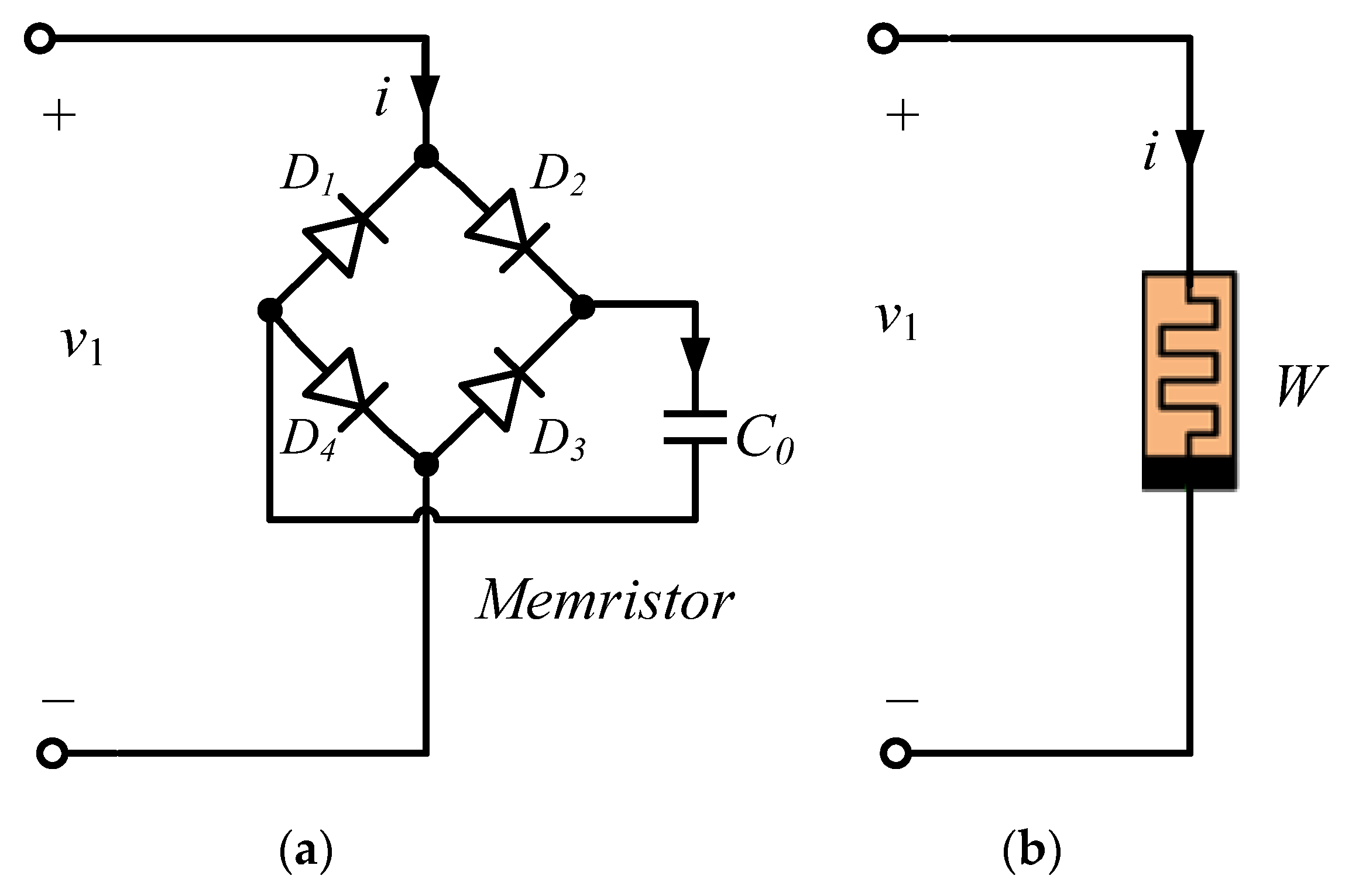
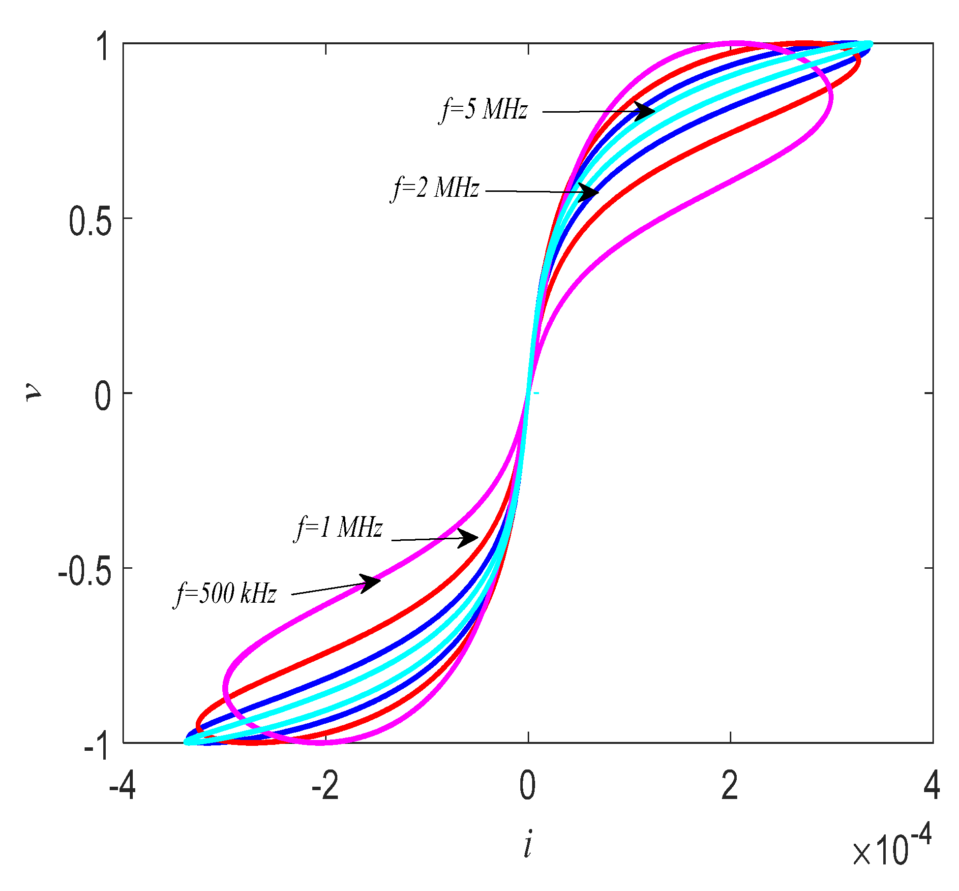
2. Generalized Memristor Emulator

Based on a first-order memristive diode bridge [22], this paper proposes a generalized memristor emulator consisting of a diode bridge with a capacitor, depicted in Figure 1. The memristor model can be expressed as:

$$\begin{array}{l}\frac{\mathrm{d}{v}_0}{\mathrm{d}t}=F(v_0,v_1)=2I_{s_0}{[\mathrm{e}}^{-\rho v_0}\cosh (\rho v_1)-1]/C_0\\ i=g(v_0,v_1)v_1=2I_{s_0}{\mathrm{e}}^{-\rho v_0}\sinh (\rho v_1)\end{array}$$

(1)

where I and v₁ are current and voltage of the memristor W, respectively, and v₀ is the voltage of the capacitor C₀, and ρ = 1/(2nV_T). Consider that the memristive emulator consists of the capacitor (C₀ = 100 pF) and the diode bridge U1B4B42, and the parameters are set as follows: reverse saturation current I_S0 = 6.543 × 10⁻⁵ A, emission coefficient n = 4.386, thermal voltage V_T = 25 mV and v = sin(2πft).

Based on (1) and the above parameters, a numerical simulation using MATLAB 2016b is shown in Figure 2. It can be observed that the area of the pinched hysteresis loop decreases monotonically as the frequency of the input voltage increases (the frequency f is 500 kHz, 1 MHz, 2 MHz and 5 MHz, respectively).

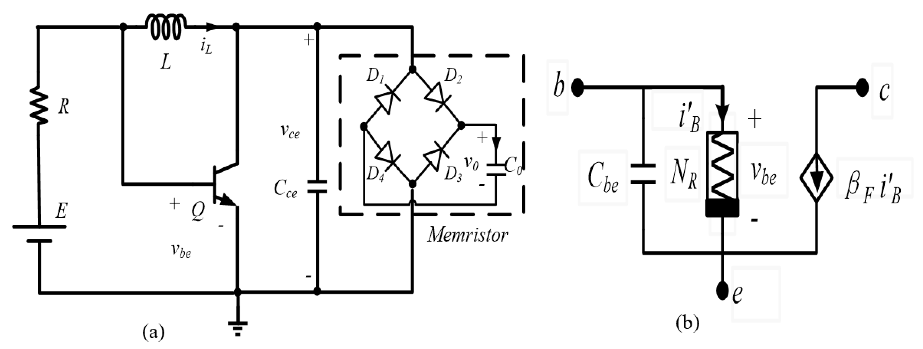
3. Memristive-Based Colpitts Circuit

The proposed memristor emulator is used in the Colpitts oscillator circuit as an application, shown in Figure 3. The small-signal high frequency model in Figure 3b of the bipolar junction transistor (BJT) in the Colpitts oscillator is used, which consists of a voltage-controlled non-linear resistor NR and a linear current-controlled current source while taking into account the parasitic capacitance C_be, where Is = 6.734 × 10⁻¹⁵ A, β_F = 416.4 and C_be = 147 pF [40].

$$i_{\mathrm{B}}{}^{\prime }=f(v_{be})=I_s{[\mathrm{e}}^{\frac{v_{be}}{V_T}}-1]/{\beta }_F$$

(2)

The memristor-based Colpitts circuit can be depicted by

$$\left\{\begin{array}{l}\frac{\mathrm{d}{v}_{ce}}{\mathrm{d}t}=\frac{i_L}{C_{ce}}-\frac{{\beta }_{F}f(v_{be})}{C_{ce}}-\frac{2I_{s_0}{\mathrm{e}}^{-\rho v_0}\sinh (\rho v_{ce})}{C_{ce}}\\ \frac{\mathrm{d}{v}_{be}}{\mathrm{d}t}=\frac{(E-v_{be})}{R{C}_{be}}-\frac{i_L}{C_{be}}-\frac{f(v_{be})}{C_{be}}\\ \frac{\mathrm{d}{i}_L}{\mathrm{d}t}=\frac{v_{be}}{L}-\frac{v_{ce}}{L}\\ \frac{\mathrm{d}{v}_0}{\mathrm{d}t}=2I_{s_0}\frac{{(\mathrm{e}}^{-\rho v_0}\cosh (\rho v_{ce})-1)}{C_0}\end{array}\right.$$

(3)

Combined with (2), (3) can be described as:

$$\left\{\begin{array}{l}\frac{\mathrm{d}{v}_{ce}}{\mathrm{d}t}=\frac{i_L}{C_{ce}}-\frac{I_s(e^{\frac{v_{be}}{V_T}}-1)}{C_{ce}}-\frac{2I_{s_0}{\mathrm{e}}^{-\rho v_0}\sinh (\rho v_{ce})}{C_{ce}}\\ \frac{\mathrm{d}{v}_{be}}{\mathrm{d}t}=\frac{(E-v_{be})}{R{C}_{be}}-\frac{i_L}{C_{be}}-\frac{I_s(e^{\frac{v_{be}}{V_T}}-1)}{C_{be}{\beta }_F}\\ \frac{\mathrm{d}{i}_L}{\mathrm{d}t}=\frac{v_{be}}{L}-\frac{v_{ce}}{L}\\ \frac{\mathrm{d}{v}_0}{\mathrm{d}t}=2I_{s_0}\frac{{(\mathrm{e}}^{-\rho v_0}\cosh (\rho v_{ce})-1)}{C_0}\end{array}\right.$$

(4)

When the left side of (4) is equal to 0, one obtains

$$\left\{\begin{array}{l}{i}_L=I_s(e^{\frac{v_{be}}{V_T}}-1)+2I_{s_0}{\mathrm{e}}^{-\rho v_0}\sinh (\rho v_{ce})\\ i_L=\frac{(E-v_{be})}{R}-\frac{I_s(e^{\frac{v_{be}}{V_T}}-1)}{{\beta }_F}\\ v_{be}=v_{ce}\\ {\mathrm{e}}^{-\rho v_0}\cosh (\rho v_{ce})=1\end{array}\right.$$

(5)

The equilibrium point can be obtained through the graphic analytic method. Based on (5), two functions describing the relationship between v_be and i_L can be depicted as:

$$\begin{array}{l}{i}_L=f_1(v_{ce})=\frac{E-v_{ce}}{R}-I_s(e^{\frac{v_{ce}}{V_T}}-1)\\ i_L=f_2(v_{ce})=2I_{s_0}\tanh (\rho v_{ce})+\frac{I_s(e^{\frac{v_{ce}}{V_T}}-1)}{{\beta }_F}\end{array}$$

(6)

when the circuit parameters are set in

Table 2. Typical circuit parameters of the memristor-based Colpitts circuit.

Parameters	Significations	Values
Cce	Capacitance	2.2 nF
L	Inductance	4.7 μH
C0	Capacitance	100 pF
E	DC voltage source	5.89 V

and the parameters of BJT are as above mentioned. Adjusting the value of the resistor (R ∈ [200, 2000]), the intersection points of v_ce and i_L curves give the solver of (6). The values of ${\widehat{v}}_{ce}$ represent the locations of the equilibrium points on the v_ce-axis, as shown in Figure 4. It can be observed that there is only one intersection point of v_ce and i_L curves with R changing. Therefore, ${\widehat{v}}_{ce}$ ∈ [0.6658, 0.7242] when R is adjusting in the range [200, 2000]. Therefore, the equilibrium point P is calculated as

$$\left({\widehat{v}}_{ce},{\widehat{v}}_{be},{\widehat{i}}_L,{\widehat{v}}_0\right)=({\widehat{v}}_{ce},{\widehat{v}}_{ce},\frac{E-{\widehat{v}}_{ce}}{R} -I_s(e^{\frac{v_{ce}}{V_T}}-1) ,-\frac{1}{\rho }\ln \frac{1}{\cosh (\rho {\widehat{v}}_{ce})})$$

(7)

For the equilibrium point P, the Jacobian matrix is yielded

$$J=\left[\begin{array}{cccc}-\frac{j_1}{C_{ce}}& -\frac{j_3}{C_{ce}}& \frac{1}{C_{ce}}& \frac{j_2}{C_{ce}}\\ 0& -\frac{1}{R{C}_{be}}-\frac{j_3}{C_{be}{\beta }_F}& -\frac{1}{C_{be}}& 0\\ -1/L& 1/L& 0& 0\\ \frac{j_2}{C_0}& 0& 0& -\frac{j_1}{C_0}\end{array}\right]$$

(8)

where $j_1=2\rho I_{s_0}{\mathrm{e}}^{-\rho v_0}\cosh (\rho v_{ce})$, $j_2=2\rho I_{s_0}{\mathrm{e}}^{-\rho v_0}\sinh (\rho v_{ce})$, $j_3=I_s{e}^{\frac{v_{be}}{V_T}}/V_T$. The dissipativity of the proposed memristive Colpitts circuit shown in Figure 3a can be derived from

$$\begin{array}{l}\nabla =\frac{\dot{\partial }{v}_{ce}}{\partial v_{ce}}+\frac{\dot{\partial }{v}_{be}}{\partial v_{be}}+\frac{\dot{\partial }{i}_L}{\partial i_L}+\frac{\dot{\partial }{v}_0}{\partial v_0}\\ =-\frac{j_1}{C_{ce}}-\frac{1}{R{C}_{be}}-\frac{j_3}{C_{be}{b}_F}-\frac{j_1}{C_0}\\ =-(\frac{j_1}{C_{ce}}+\frac{1}{R{C}_{be}}+\frac{j_3}{C_{be}{b}_F}+\frac{j_1}{C_0})\end{array}$$

(9)

The negative exponential function, exponential function, hyperbolic cosine function and system parameters are always positive; therefore, ∇ < 0, and the system (3) is dissipation.

The corresponding characteristic equation is expressed as

$$\det (\lambda I-J)=0$$

(10)

Table 3. Equilibrium point and eigenvalues under different values of R.

R/Ω	Equilibrium Point P	Eigenvalues
200	(0.7242, 0.7242, 0.0002, 0.5725)	${\lambda }_1=-10.159\times {10}^7\hspace{1em}{\lambda }_{2,3}=(2.528 \pm 7.780i)\times {10}^7\hspace{1em}{\lambda }_4=-0.596\times {10}^7$
500	(0.7012, 0.7012, 0.0104, 0.5496)	${\lambda }_{1,2}= (2.1464 \pm 6.1750i )\times {10}^7\hspace{1em}{\lambda }_3=-6.3494\times {10}^7\hspace{1em}{\lambda }_4=-0.5959\times {10}^7$
800	(0.6893, 0.6893, 0.0001, 0.5377)	${\lambda }_{1,2}=(1.8463\pm 5.5196i )\times {10}^7 {\lambda }_3=-4.9868\times {10}^7 {\lambda }_4=-0.5953\times {10}^7$
1200	(0.6790, 0.6790, 0.0001, 0.5274)	${\lambda }_{1,2}= (1.5642 \pm 5.0511 i )\times {10}^7 {\lambda }_3=-3.9993\times {10}^7 {\lambda }_4=-0.5945\times {10}^7$
2000	(0.6658, 0.6658, 0.0001, 0.5143)	${\lambda }_{1,2}=(1.2025 \pm 4.5890i )\times {10}^7 {\lambda }_3=-2.9383\times {10}^7 {\lambda }_4=-0.5926\times {10}^7$

summarizes the equilibrium point P and the eigenvalues under different values of R.

Obviously, there are two negative real roots and two complex conjugate roots with positive real part at P, indicating that P has two unstable saddle-foci with index 2, leading to the occurrence of chaos.

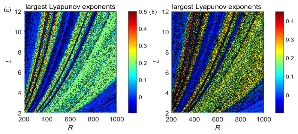
4. Complex Dynamical Behaviors

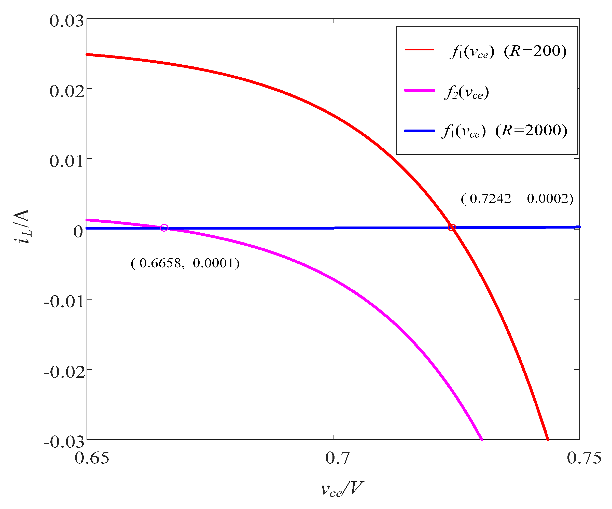
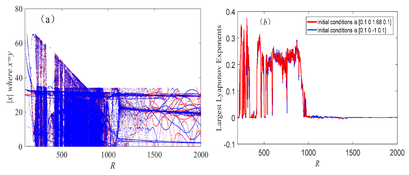
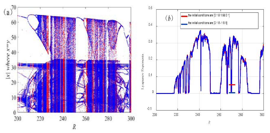
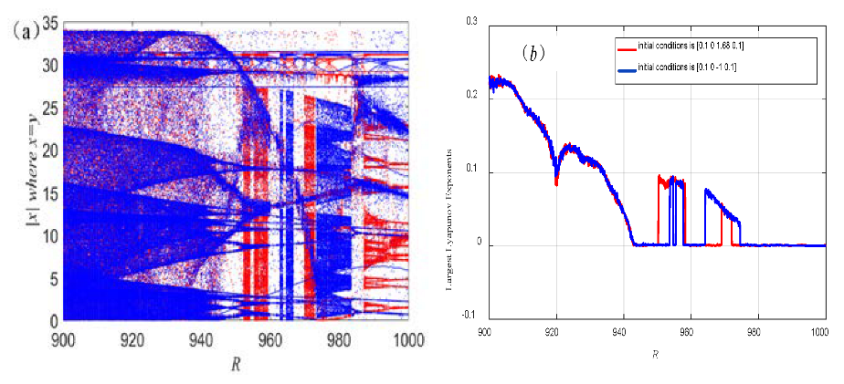
4.1. Phase Portraits with Respect to Variables R

In order to demonstrate the complex dynamical behaviors of system model (4), we choose parameter values as follows: Is = 6.734 × 10⁻¹⁵ A, β_F = 416.4, C_be = 147 pF, C₀ = 100 pF, I_S0 = 6.543 × 10⁻⁵ A, n = 4.386, V_T = 25 mV, E = 5.89, C_ce = 2.2 nF, and L = 4.7 μH. The Runge–Kutta algorithm (ode23) is utilized, and the initial conditions are [0.1, 0, −1, 0.1]. The phase portraits are depicted in Figure 5; it can be observed that there exist various types of chaotic and periodic orbits with the change in its parameter R, and they reflect the complexity of system model (4). Further extensions to dynamical behavior analyze the basins of attraction in the next section.

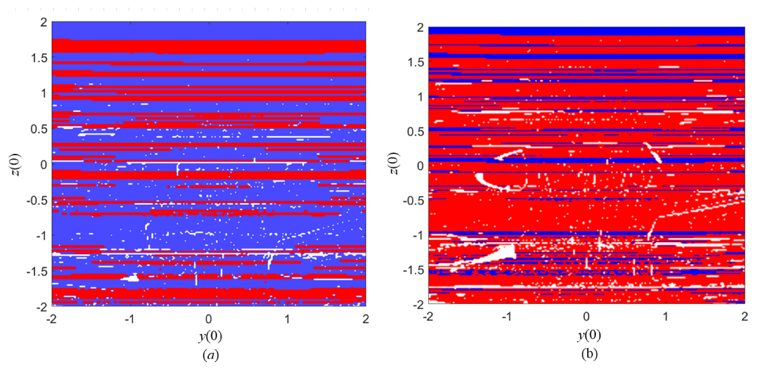
4.2. Basins of Attraction

More information about coexisting attractors can be acquired by investigating basins of attraction of different attracting sets. Based on the method in [30], we calculate the local basin of attraction of system model (4).

Keeping the parameters fixed as shown in Section 4.1 and adjusting R, the attraction basins in the y(0)–z(0) initial plane are plotted in Figure 6. The adjustable initial conditions y₀ and z₀ are all scanned in the region of [–2, 2]. Figure 6 uses the different color (red and blue) to intuitively mean two kinds of coexisting attractors in the system model (4), while white zones denote unbounded motion.

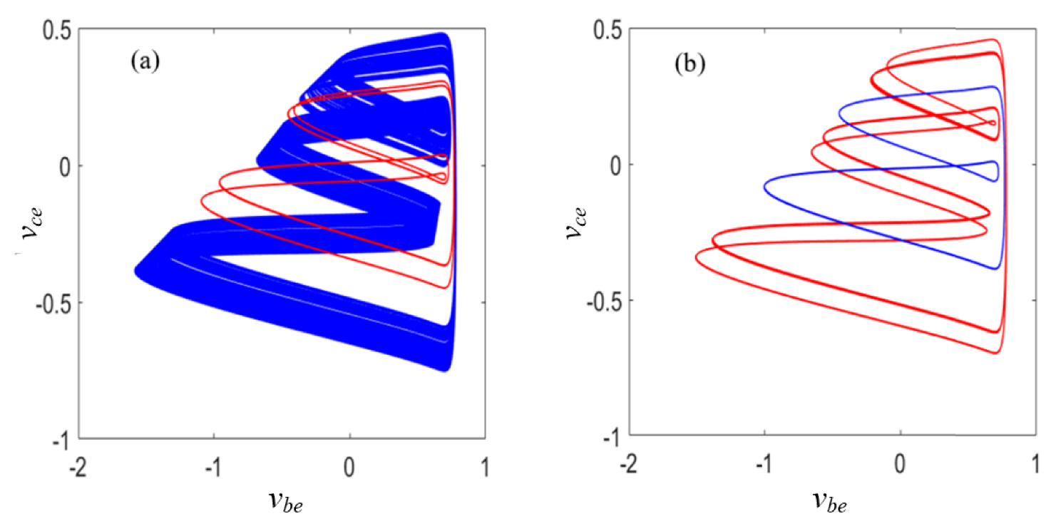
4.3. Coexisting Multiple Attractors

The coexisting multiple attractors reveal a rich diversity of stable states in nonlinear systems [25]. Under certain parameters, different initial conditions may lead to different trajectories of the system. Based on the above basin of attraction, we choose some initial conditions to draw phase portraits of system model (4).

According to the analysis of basins of attraction in Section 4.1, we choose two initial conditions (0.1, 0, −1, 0.1) and (0.1, 0, 1.68, 0.1). The phase portraits in the v_be–v_ce plane for different initial conditions are illustrated in Figure 7. There exists a chaotic attractor with tridentate structure and periodic-2 orbits with bicuspid structure (R = 966), as shown in Figure 7a. There exist period-1 orbits with bicuspid structure and periodic-2 orbits with tridentate structure (R = 1000), as shown in Figure 7b.

To explore the nonlinear dynamics caused by the memristor, we compute the bifurcation diagram and the largest Lyapunov exponent as R increases from 200 to 2000; bifurcation diagrams and the corresponding largest Lyapunov exponent are shown in Figure 8. Obviously, the bifurcation diagram and the largest Lyapunov exponent are well-consistent with each other. Two different moving trajectories are presented in Figure 8 when the initial conditions are [0.1, 0, 1.68, 0.1] (Red) and [0.1, 0, −1, 0.1] (Blue). With respect to the increase in the system parameter R (R ∈ [200, 952]), the trajectory of the red motion and the blue motion are overlapped except for a few discrete points indicating unbounded motion. In order to observe the local details, Figure 9 is the enlargement of Figure 8 (R ∈ [200, 300]). By observing the trajectory of the motion in Figure 9, it can be observed that the system is period-1 orbits at R = 200, period-2 orbits at R = 209 and period-4 orbits at R = 216, then enters the chaotic state at R = 218 through the period-doubling bifurcation. It is worth mentioning that in Figure 9a, some evident period windows exist within the chaotic region, which is caused by chaos crisis and ended by tangential bifurcation [11], such as R ∈ [221.3, 221.8], R ∈ [222, 222.3], R ∈ [227.4, 228.6], R ∈ [267.3, 267.8], R ∈ [271.3, 271.8] and R = 277.2. Then the state degrades from chaos to period-2 (R = 288) and transforms into period-1 orbits (R = 191.6) from the reverse period-doubling bifurcation. When v > 952, the system exists in coexisting bifurcations as shown in Figure 10a. Figure 10 is the enlargement of Figure 8 (R ∈ [900, 1000]).

A two-parameter Lyapunov exponent is drawn using the control parameters R (200 ≤ R ≤ 1000) and L (2 ≤ L ≤ 12), and the other parameters are unchanged in Section 4.1. Sample results under the initial conditions [0.1 0 −1 0.1] and [0.1 0 1.68 0.1] are described in Figure 11a,b, respectively. Each color represents different values of the largest Lyapunov exponents (refer to the colorbar on the right for details), while white zones denote that the largest Lyapunov exponent is NaN (not a number). At the corresponding value of R and L, the system model (4) under the different conditions has different largest Lyapunov exponents, and it furtherly indicates that the proposed circuit can exhibit rich dynamical behaviors.

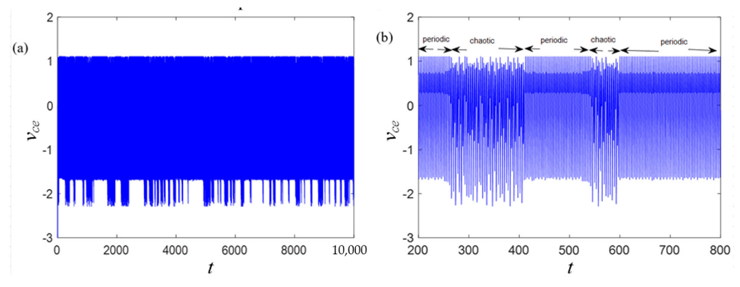
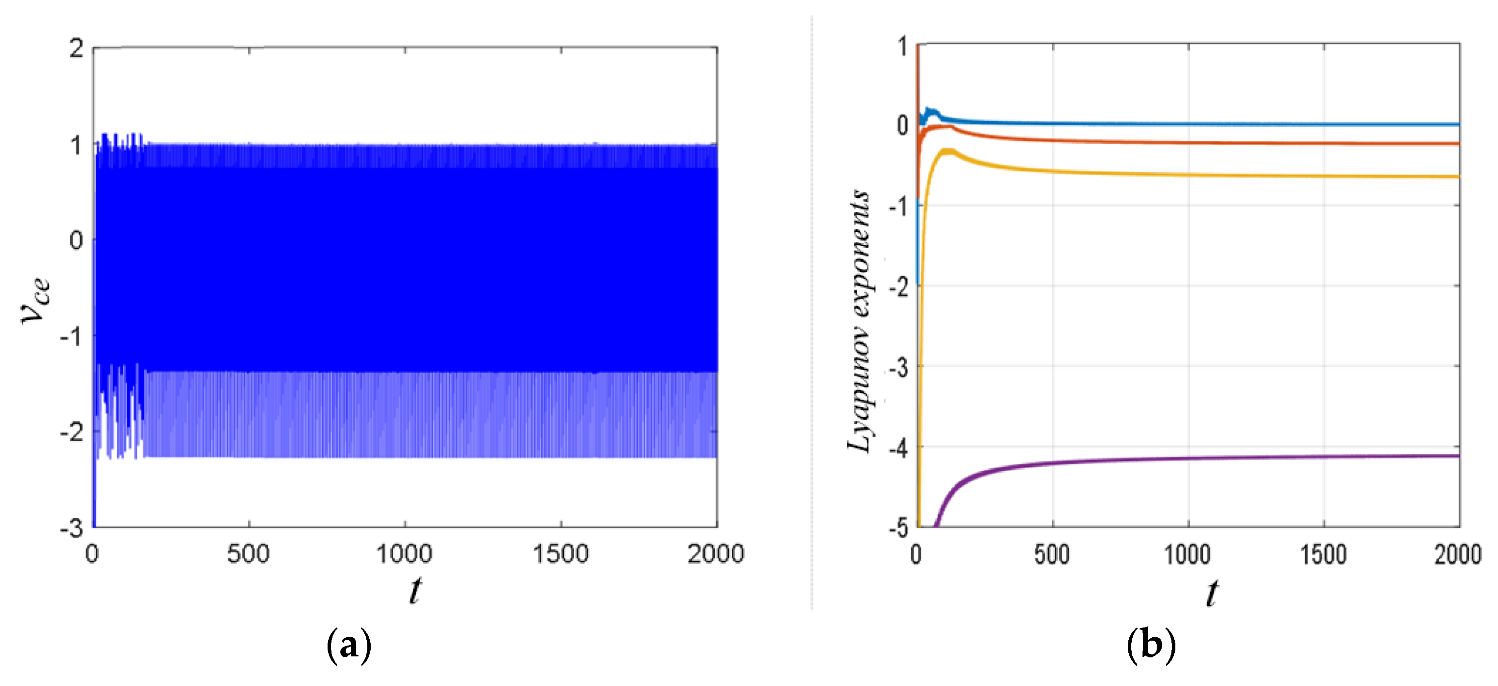
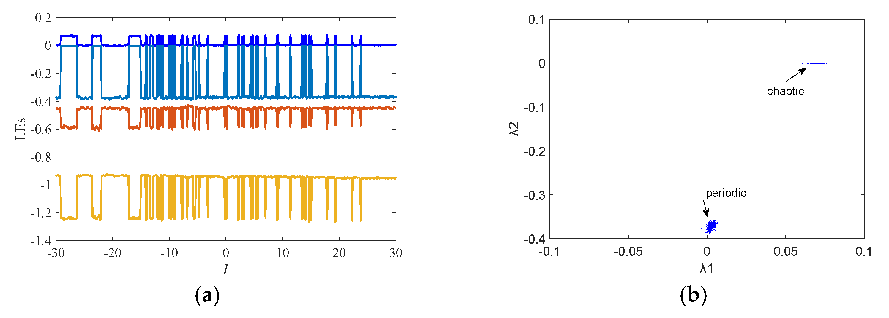
4.4. Intermittent Chaos and Transient Chaos

The irregular alternation of periodic and chaotic is known as intermittency, which is caused by an interior crisis. The time-domain waveform of state variable v_ce is shown in Figure 12. Figure 12b is the enlargement of Figure 12a; it can be seen that it alternates between chaotic orbits and periodic orbits.

Transient chaos describes the chaotic behaviors of the system on a finite time scale, and ultimately evolves into regular behaviors such as fixed point or periodic orbit. The time-domain waveform of state variable v_ce is chaotic in t ∈ [0, 120], and periodic in t ∈ [120, 2000], as shown in Figure 13a. According to [41], the time Lyapunov exponent spectrums are shown in Figure 13b.

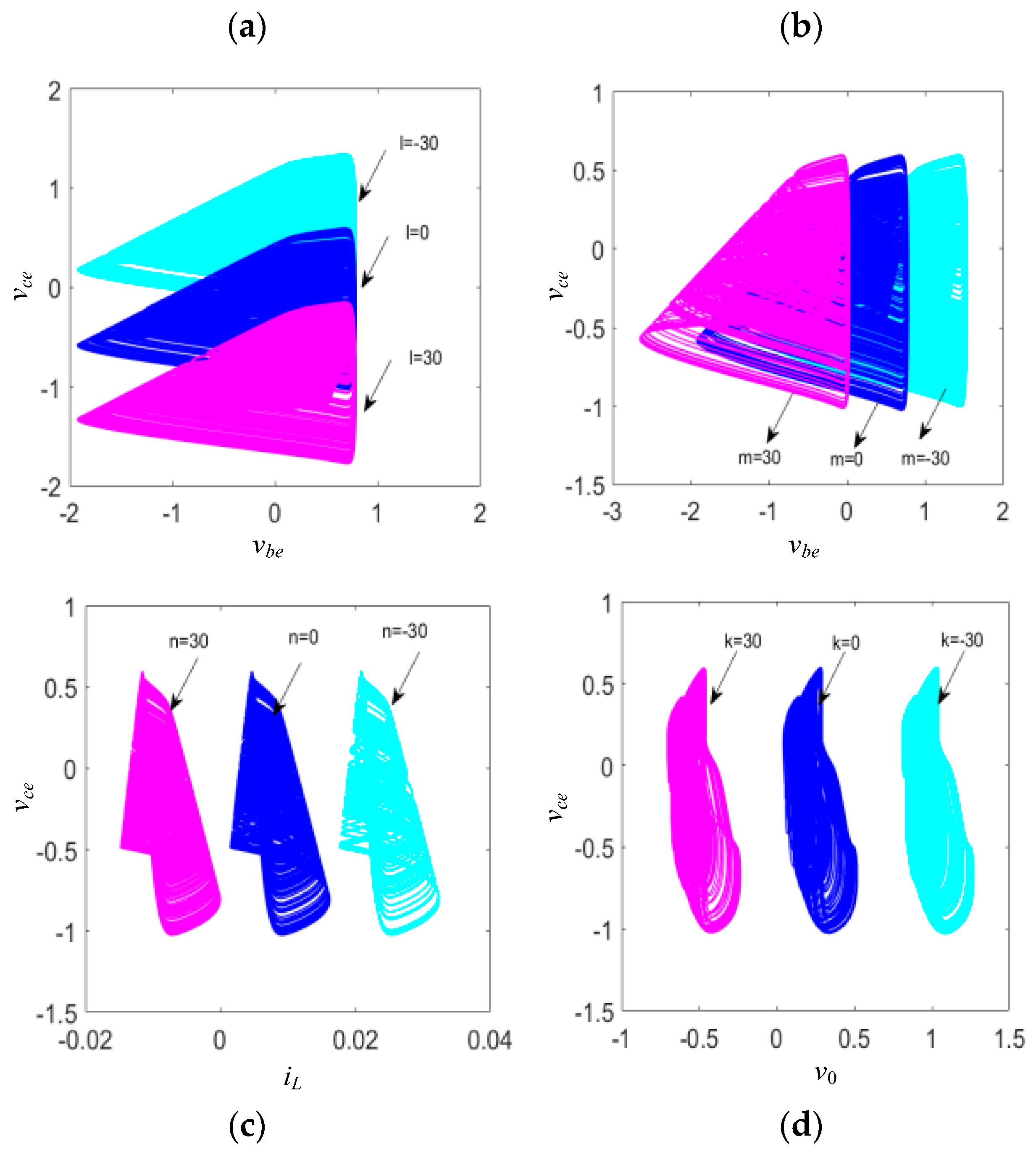
4.5. Offset Boosting

It is universally acknowledged that some chaotic systems exist with an interesting offset boosting property that may be used for amplitude control [42].

The parameters are expressed as follows:

$$\begin{array}{l}{v}_{ce}=x{V}_T, v_{be}=y{V}_T, i_L=z{V}_T/q,v_0=u{V}_T,t=\tau \sqrt{L{C}_{ce}},q=\sqrt{L/C_{ce}},\\ a=q{I}_s/V_T,\alpha =2q{I}_{s_0}/V_T,b=C_{ce}/C_{be},c=q/R,d=C_{ce}/C_0,e=E/V_T\end{array}$$

(11)

Therefore, the dimensionless equations can be described as follows:

$$\left\{\begin{array}{l}\dot{x}=z-a(e^y-1)-\alpha {\mathrm{e}}^{-u/2n}\sinh (x/2n)\\ \dot{y}=b(c(e-y)-z-a(e^y-1)/{\beta }_F)\\ \dot{z}=y-x\\ \dot{u}=\alpha d{(\mathrm{e}}^{-u/2n}\cosh (x/2n)-1)\end{array}\right.$$

(12)

By introducing four extra controlled constants l, m, n and k to variables x, y, z and u, respectively, the system (12) can be expressed by

$$\left\{\begin{array}{l}\dot{x}=(z+n)-a(e^{(y+m)}-1)-\alpha {\mathrm{e}}^{-(u+k)/2n}\sinh ((x+l)/2n)\\ \dot{y}=b(c(e-(y+m))-(z+n)-a{I}_s(e^{(y+m)}-1)/{\beta }_F)\\ \dot{z}=(y+m)-(x+l)\\ \dot{u}=\alpha d{(\mathrm{e}}^{-(u+k)/2n}\cosh ((x+l)/2n)-1)\end{array}\right.$$

(13)

where l, m, n and k are the real numbers. The other parameter values are the same as in Section 4.1 and R = 800; the values of a, b, c, d and e can be calculated using (11).

To better clarify the offset boosting behavior, different l, m, n and k are chose to plot the phase portraits. Offset boosting behaviors with varying control parameter l, m, n and k are can be captured in Figure 14 when the initial conditions are (0.1, 0, −1, 0.1). It is found that the attractors are respectively boosted towards the x, y, z and u direction.

In order to analyze the multistability, the novel non-invasive method of offset [43] was exploited. The parameter values are the same as in Section 4.1 and R = 966. Let offset boosting be applied to variable x, as shown below:

$$\left\{\begin{array}{l}\dot{x}=z-a(e^y-1)-2\alpha {\mathrm{e}}^{-u/2n}\sinh ((x+l)/2n)\\ \dot{y}=b(c(e-y)-z-a{I}_s(e^y-1)/{\beta }_F)\\ \dot{z}=y-(x+l)\\ \dot{u}=2\alpha d{(\mathrm{e}}^{-u/2n}\cosh ((x+l)/2n)-1)\end{array}\right.$$

(14)

When the initial conditions are [0.1, 0, −1, 0.1] and [0.1, 0, 1.68, 0.1], the dynamical behaviors of System (14) versus offset booster l (l ∈ [−30, 30]) are plotted in Figure 15 and Figure 16. The results are a further proof of the coexistence of two different properties of dynamics.

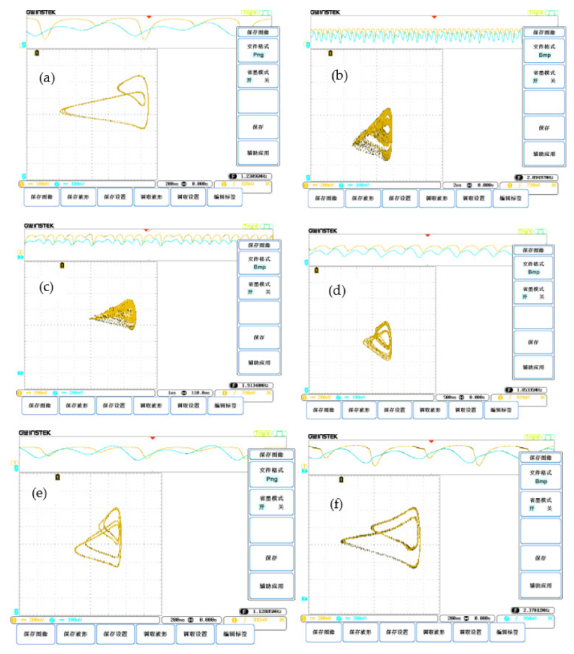
5. Hardware Experiments

In order to further research the proposed memristive system shown in Figure 3, hardware experiments on a breadboard containing a potentiometer, inductance, capacitor, diode bridge U1B4B42, bipolar junction transistor 2N222 and DC voltage source were conducted to verify dynamical behaviors of the proposed oscillator. In the experimental circuit, the element parameters are measured and shown as Table 2. R is a variable resistance. The experimental circuit in operation is captured in Figure 17. The FFT function of the oscilloscope is exploited to analyze the power spectrum. The power spectrums are depicted in Figure 18, and it can be observed that the frequencies are in the range of MegaHertz. The experimental results are photographed using GDS2102a, as shown in Figure 19. The oscilloscope traces from the proposed memristive Colpitts circuit in Figure 19 are similar to Figure 6. Based on frequencies displayed on the oscilloscope interface, it is evidenced that the proposed memristive Colpitts oscillator operates in high frequency.

6. Conclusions

This paper reports a memristive emulator with higher frequency that is composed of a diode bridge and a capacitor. The mathematical modeling and MATLAB simulations are presented in detail. Then a memristor-based Colpitts oscillator is constructed, and simulations and experiment circuit results show the system has complex dynamic behaviors. This study further verifies the realizability of the proposed memristor model and its potential application value in the field of secure communication.

References

1. Chua, L. Memristor-The missing circuit element. IEEE Trans. Circuit Theory 1971, 18, 507–519. [Google Scholar] [CrossRef]
2. Strukov, D.B.; Snider, G.S.; Stewart, D.R.; Williams, R.S. The missing memristor found. Nature 2008, 453, 80–83. [Google Scholar] [CrossRef]
3. Khalid, M.; Singh, J. Memristor based unbalanced ternary logic gates. Anal. Integr. Circuits Signal Process. 2016, 87, 399–406. [Google Scholar] [CrossRef]
4. Wang, X.; Zhou, P.; Eshraghian, J.; Lin, C.; Iu, H.; Chang, T. High-Density Memristor-CMOS Ternary Logic Family. IEEE Trans. Circuits Syst. I Regul. Pap. 2021, 68, 264–274. [Google Scholar] [CrossRef]
5. Liu, P.; You, Z.; Wu Ji Liu, B.; Han, Y.; Chakrabarty, K. Fault Modeling and Efficient Testing of Memristor-Based Memory. IEEE Trans. Circuits Syst. I Regul. Pap. 2021, 11, 4444–4455. [Google Scholar] [CrossRef]
6. Parshina, L.; Novodvorsky, O.; Khramova, O.; Gusev, D.; Polyakov, A.; Mikhalevsky, V.; Cherebilo, E. Laser synthesis of non-volatile memristor structures based on tantalum oxide thin films. Chaos Solitons Fractals 2021, 142, 110460. [Google Scholar] [CrossRef]
7. Bharathi, M.; Wang, Z.; Guo, B.; Balraj, B.; Li, Q.; Shuai, J.; Guo, D. Memristors: Understanding, utilization and upgradation for neuromorphic computing. Nano 2020, 15, 15. [Google Scholar] [CrossRef]
8. Li, Y.; Ang, K.W. Hardware Implementation of Neuromorphic Computing Using Large-Scale Memristor Crossbar Arrays. Adv. Intell. Syst. 2021, 3, 2000137. [Google Scholar] [CrossRef]
9. Li, Z.; Zhou, H.; Wang, M.; Ma, M. Coexisting firing patterns and phase synchronization in locally active memristor coupled neurons with HR and FN models. Nonlinear Dyn. 2021, 104, 1455–1473. [Google Scholar] [CrossRef]
10. Lin, H.; Wang, C.; Xu, C.; Zhang, X.; Iu, H.H.C. A Memristive Synapse Control Method to Generate diversified multistructure chaotic attractor. IEEE Trans. Comput. Aided Des. Integr. Circuits Syst. 2022, 1. [Google Scholar] [CrossRef]
11. Wan, Q.; Yan, Z.; Li, F.; Chen, S.; Liu, J. Complex dynamics in a Hopfield neural network under electromagnetic induction and electromagnetic radiation. Chaos 2022, 32, 073107. [Google Scholar] [CrossRef]
12. Lin, H.; Wang, C.; Cui, L.; Sun, Y.; Xu, C.; Yu, F. Brain-like initial-boosted hyperchaos and application in biomedical image encryption. IEEE Trans. Ind. Inform. 2022, 18, 8839–8850. [Google Scholar] [CrossRef]
13. Ran, H.; Wen, S.; Li, Q.; Yang, Y.; Shi, K.; Feng, Y.; Zhou, P.; Huang, T. Memristor-Based Edge Computing of Blaze Block for Image Recognition. IEEE Trans. Neural Netw. Learn. Syst. 2020, 33, 2121–2131. [Google Scholar] [CrossRef] [PubMed]
14. Zhao, H.; Liu, Z.; Tang, J.; Gao, B.; Zhang, Y.; Qian, H.; Wu, H. Memristor-Based Signal Processing for Edge Computing. Tsinghua Sci. Technol. 2022, 27, 455–471. [Google Scholar] [CrossRef]
15. Li, C.; Li, H.; Xie, W.; Du, J. A S-type bistable locally active memristor model and its analog implementation in an oscillator circuit. Nonlinear Dyn. 2021, 1, 1041–1058. [Google Scholar] [CrossRef]
16. Xie, W.; Wang, C.; Lin, H. A fractional-order multistable locally active memristor and its chaotic system with transient transition, state jump. Nonlinear Dyn. 2021, 104, 4523–4541. [Google Scholar] [CrossRef]
17. Ma, M.; Yang, Y.; Qiu, Z.; Peng, Y.; Sun, Y.; Li, Z.; Wang, M. A locally active discrete memristor model and its application in a hyperchaotic map. Nonlinear Dyn. 2022, 107, 2935–2949. [Google Scholar] [CrossRef]
18. Knowm Inc. Products. Available online: https://knowm.com/collections/all/ (accessed on 26 May 2020).
19. Yesil, A. A New Grounded Memristor Emulator Based on MOSFET-C. AEU-Int. J. Electron. Commun. 2018, 91, 143–149. [Google Scholar] [CrossRef]
20. Vista, J.; Ranjan, A. A Simple Floating MOS-Memristor for High-Frequency Applications. IEEE Trans. Very Large Scale Integr. Syst. 2019, 27, 1186–1195. [Google Scholar] [CrossRef]
21. Ghosh, M.; Singh, A.; Borah, S.S.; Vista, J.; Ranjan, A.; Kumar, S. MOSFET-Based Memristor for High-Frequency Signal Processing. IEEE Trans. Electron. Devices 2022, 69, 2248–2255. [Google Scholar] [CrossRef]
22. Corinto, F.; Ascoli, A. Memristive diode bridge with LCR filter. Electron. Lett. 2012, 48, 824–825. [Google Scholar] [CrossRef]
23. Bao, B.C.; Yu, J.J.; Hu, F.W. Generalized memristor consisting of diode bridge with first order parallel RC filter. Int. J. Bifurc. Chaos 2014, 24, 1350143. [Google Scholar] [CrossRef]
24. Wu, H.G.; Bao, B.C.; Liu, Z.; Xu, Q.; Jiang, P. Chaotic and periodic bursting phenomena in a memristive Wien-bridge oscillator. Nonlinear Dyn. 2015, 83, 893–903. [Google Scholar] [CrossRef]
25. Bao, B.C.; Xu, L.; Wu, Z.M.; Chen, M.; Wu, H.G. Coexistence of multiple bifurcation modes in memristive diode-bridge based canonical Chua’s circuit. Int. J. Electron. 2018, 105, 1159–1169. [Google Scholar] [CrossRef]
26. Kengne, J.; Leutcho, G.D.; Telem, A. Reversals of period doubling, coexisting multiple attractors, and offset boosting in a novel memristive diode bridge-based hyperjerk circuit. Analog. Integr. Circuits Signal Process. 2019, 101, 379–399. [Google Scholar] [CrossRef]
27. Chithra, A.; Fozin, T.F.; Srinivasan, K.; Kengne, E.R.M.; Kouanou, A.T.; Mohamed, I.R. Complex Dynamics in a Memristive Diode Bridge-Based MLC Circuit: Coexisting Attractors and Double-Transient Chaos. Int. J. Bifurc. Chaos 2021, 31, 2150049. [Google Scholar] [CrossRef]
28. Wang, N.; Zhang, G.; Bao, H. Bursting oscillations and coexisting attractors in a simple memristor-capacitor-based chaotic circuit. Nonlinear Dyn. 2019, 97, 1477–1494. [Google Scholar] [CrossRef]
29. Li, F.; Tai, C.; Bao, H.; Luo, J.; Bao, B. Hyperchaos, quasi-period and coexisting behaviors in second-order-memristor-based jerk circuit. Eur. Phys. J. Spec. Top. 2020, 229, 1045–1058. [Google Scholar] [CrossRef]
30. Kengne, L.K.; Pone, J.; Hilaire, F. On the dynamics of chaotic circuits based on memristive diode-bridge with variable symmetry: A case study. Chaos Solitons Fractals 2021, 145, 110795. [Google Scholar] [CrossRef]
31. Wu, H.; Zhou, J.; Chen, M.; Xu, Q.; Bao, B. DC-offset induced asymmetry in memristive diode-bridge-based Shinriki oscillator. Chaos Solitons Fractals 2022, 154, 111624. [Google Scholar] [CrossRef]
32. Ramadoss, J.; Kengne, J.; Telem AN, K.; Rajagopal, K. Broken symmetry and dynamics of a memristive diodes bridge-based Shinriki oscillator. Phys. A Stat. Mech. Its Appl. 2022, 588, 126562. [Google Scholar] [CrossRef]
33. Sánchez-López, C. RuizBharathwaj Muthuswamy. Implementing Memristor Based Chaotic Circuits. Int. J. Bifurc. Chaos 2010, 20, 1002651. [Google Scholar]
34. Kim, H.; Sah, M.P.; Yang, C.; Cho, S.; Chua, L.O. Memristor Emulator for Memristor Circuit Applications. IEEE Trans. Circuits Syst. I Regul. Pap. 2012, 59, 2422–2431. [Google Scholar]
35. Yesil, A.; Babacan, Y.; Kacar, F. A new DDCC based memristor emulator circuit and its applications. Microelectron. J. 2014, 45, 282–287. [Google Scholar] [CrossRef]
36. Sánchez-López, C.; Aguila-Cuapio, L.E. A 860 kHz grounded memristor emulator circuit. AEUE-Int. J. Electron. Commun. 2017, 73, 23–33. [Google Scholar] [CrossRef]
37. Ranjan, R.K.; Rani, N.; Pal, R.; Paul, S.K.; Kanyal, G. Single CCTA based high frequency floating and grounded type of incremental/decremental memristor emulator and its application. Microelectron. J. 2017, 60, 119–128. [Google Scholar] [CrossRef]
38. Vista, J.; Ranjan, A. Flux Controlled Floating Memristor Employing VDTA: Incremental or Decremental Operation. IEEE Trans. Comput.-Aided Des. Integr. Circuits Syst. 2021, 40, 364–372. [Google Scholar] [CrossRef]
39. Raj, A.; Singh, S.; Kumar, P. Dual mode, high frequency and power efficient grounded memristor based on OTA and DVCC. Analog. Integr. Circuits Signal Process. 2022, 110, 81–89. [Google Scholar] [CrossRef]
40. Tekam, B.; Kengne, J.; Kenmoe, G.D. High frequency Colpitts’ oscillator: A simple configuration for chaos generation. Chaos Solitons Fractals 2019, 126, 351–360. [Google Scholar] [CrossRef]
41. Sabarathinam, S.; Thamilmaran, K. Transient chaos in a globally coupled system of nearly conservative Hamiltonian Duffing oscillators. Chaos Solitons Fractals 2015, 73, 129–140. [Google Scholar] [CrossRef]
42. Li, C.; Gu, Z.; Liu, Z.; Jafari, S.; Kapitaniak, T. Constructing chaotic repellors. Chaos Solitons Fractals 2021, 42, 110544. [Google Scholar] [CrossRef]
43. Li, C.; Xiong, W.; Chen, G. Diagnosing multistability by offset boosting. Nonlinear Dyn. 2017, 90, 1335–1341. [Google Scholar] [CrossRef]
Figure 1. Generalized memristor (a) diode bridge with parallel C; (b) symbol of memristor.
Mathematics 10 04820 g001
Figure 2. Pinched hysteresis loop of the generalized memristor driven by input voltages with different frequency (in MATLAB).
Mathematics 10 04820 g002
Figure 3. Memristor-based Colpitts circuit. (a) Memristor-based Colpitts circuit; (b) the BJT model used for the analysis.
Mathematics 10 04820 g003
Figure 4. vce and iL curves and their intersection points.
Mathematics 10 04820 g004
Figure 5. Phase portraits of the proposed system with respect to variables R: (a) R = 200; (b) R = 230; (c) R = 830; (d) R = 935; (e) R = 960; (f) R = 1000.
Mathematics 10 04820 g005
Figure 6. Basins of attraction in the y(0)–z(0) initial plane with [0.1, y(0), z(0), 0.1]: (a) R = 1000 (b) R = 966.
Mathematics 10 04820 g006
Figure 7. Phase portraits in the vbe–vce plane for different initial conditions: (a) R = 966; (b) R = 1000.
Mathematics 10 04820 g007
Figure 8. Dynamic behaviors of the proposed system with respect to variables R: (a) bifurcation diagram, (b) largest Lyapunov exponent.
Mathematics 10 04820 g008
Figure 9. The enlargement of Figure 8 (R ∈ [200, 300]): (a) bifurcation diagram, (b) largest Lyapunov exponent.
Mathematics 10 04820 g009
Figure 10. The enlargement of Figure 8 (R ∈ [900, 1000]): (a) bifurcation diagram, (b) largest Lyapunov exponent.
Mathematics 10 04820 g010
Figure 11. Diagram of maximal Lyapunov exponents with different initial condition: (a) [0.1 0 −1 0.1] (b) [0.1 0 1.68 0.1].
Mathematics 10 04820 g011
Figure 12. Time-domain waveform of vce when R = 228.6 and the initial conditions are [0.1, 0, −1, 0.1]: (a) t ∈ [0, 10,000], (b) t ∈ [200, 800].
Mathematics 10 04820 g012
Figure 13. Dynamical behaviors when R = 231 and the initial conditions are [0.1, 0, −1, 0.1] (a) time-domain waveform of vce, (b) Lyapunov exponent spectrums versus t.
Mathematics 10 04820 g013
Figure 14. Offset boosting of chaotic attractors for varying the control parameter. (a) l = 0 and l = ±30, (b) m = 0 and m = ±30, (c) n = 0 and n = ±30 and (d) k = 0 and k = ±30.
Mathematics 10 04820 g014
Figure 15. Dynamical behaviors of System (14) on the initial condition (0.1, 0, −1, 0.1) versus offset booster l (l ∈ [−30, 30]): (a) Lyapunov exponent spectrums, (b) distribution of Lyapunov exponents.
Mathematics 10 04820 g015
Figure 16. Dynamical behaviors of System (14) on the initial condition (0.1, 0, 1.68, 0.1) versus offset booster l (l ∈ [−30, 30]): (a) Lyapunov exponent spectrums, (b) distribution of Lyapunov exponents.
Mathematics 10 04820 g016
Figure 17. The photo of experimental circuit in operation.
Mathematics 10 04820 g017
Figure 18. The power spectrum of chaotic attractors captured by Figure 17. The Chinese characters on the right of the figure means (from top to down): save image, file format Bmp, Ink-saving mode (open, off), save, and assistant function; The Chinese characters on the bottom of the figure means (from left to right): save image, save waveform, save setting, modulate waveform, and edit tag.
Mathematics 10 04820 g018
Figure 19. Phase portraits in the vbevce plane observed from oscilloscope. For each subfigure, the Chinese characters on the right of the figure means (from top to down): save image, file format Bmp, Ink-saving mode (open, off), save, and assistant function; The Chinese characters on the bottom of the figure means (from left to right): save image, save waveform, save setting, modulate waveform, and edit tag.
Mathematics 10 04820 g019