Article

Adaptive Distributed Parallel Training Method for a Deep Learning Model Based on Dynamic Critical Paths of DAG

1
School of Computing Science, Hangzhou Danzi University, Hangzhou 310018, China
2
Key Laboratory for Modeling and Simulation of Complex Systems, Ministry of Education, Hangzhou 310018, China
3
Data Security Governance Zhejiang Engineering Research Center, Hangzhou 310018, China
*
Authors to whom correspondence should be addressed.
Mathematics 2022, 10(24), 4788; https://doi.org/10.3390/math10244788
Submission received: 21 November 2022 / Revised: 10 December 2022 / Accepted: 13 December 2022 / Published: 16 December 2022

Abstract

:
AI provides a new method for massive simulated data calculations in molecular dynamics, materials, and other scientific computing fields. However, the complex structures and large-scale parameters of neural network models make them difficult to develop and train. The automatic parallel technology based on graph algorithms is one of the most promising methods to solve this problem, despite the low efficiency in the design, implementation, and execution of distributed parallel policies for large-scale neural network models. In this paper, we propose an adaptive distributed parallel training method based on the dynamic generation of critical DAG (directed acyclic graph) paths, called FD-DPS, to solve this efficiency problem. Firstly, the proposed model splits operators with the dimension of the tensor, which can expand the space available for model parallelism. Secondly, a dynamic critical path generation method is employed to determine node priority changes in the DAG of the neural network models. Finally, the model implements the optimal scheduling of critical paths based on the priority of the nodes, thereby improving the performance of parallel strategies. Our experiments show that FD-DPS can achieve 12.76% and 11.78% faster training on PnasNet_mobile and ResNet_200 models, respectively, compared with the MP-DPS and Fast methods.

1. Introduction

AI technology is gradually being applied to scientific computing scenarios that need to deal with massive amounts of data, such as molecular dynamics, materials, petroleum, gene sequencing, and whole-brain computing simulations. AI technology provides a new method for scientific computing. For example, it has high accuracy in calculating inter-atomic interaction forces using first-principles density functional theory (DFT), but it can only handle a water system with 1000 atoms [1,2]. Lu et al. [3] proposed the DeepMD-kit model, which can handle a water system with up to 1 billion atoms using AI. In biology, Jumper et al. [4] proposed AlphaFold to predict protein structures. Their model obtained an accuracy of 98% whereas the traditional co-evolutionary algorithm (co-evolution) [5] obtains a prediction accuracy of only 83%. It can, therefore, be seen that deep learning methods can effectively process massive amounts of data in molecular dynamics, protein simulation, and other scientific computing scenarios.
However, the complex structure and large-scale parameters of deep learning models present serious challenges. The number of parameters in a deep learning model can reach hundreds of millions or even trillions; for example, Alphfold [4] has 2100 million parameters, ESMFold [6] has 15 billion parameters, and GPT-3 [7] has 175 billion parameters. With limited resources, a single device cannot handle models of this size. Distributed parallel technology using multiple devices has become a popular method for training large-scale deep learning models. It divides the large-scale model into multiple submodels and then assigns these submodels to multiple devices for parallel execution. This process is called Model Parallelism. At present, the design and implementation of model parallelism mainly rely on expert experience. For example, Wu et al. [8] and Sutskever et al. [9] proposed a model parallelism method that splits a model into partitions horizontally and vertically across layers and then processes each partition on different devices. Sun et al. [10] utilized an explore–exploit framework to divide the DNNs dynamically. Ballard et al. [11] adopted a tensor segmentation method to implement intra-node parallelism. For these methods, we need to redesign the implementation of the model parallelism method when the model architecture or device environment changes. In addition, these methods need a lot of field experience and time.
In order to improve the efficiency of model parallelism, including the efficiency of design, implementation, and execution of deep learning models, many researchers have proposed auto-parallel methods, which can automatically search and tune the distributed parallel strategies and provide end-to-end adaptive distributed training solutions for deep learning models. There are two main types of auto-parallel methods: one is the auto-parallel method based on machine learning, such as Placeto [12], HeterPS [13], RIFLING [14], etc., and the other is the auto-parallel methods based on graph algorithms, such as TensorOpt [15], Alpa [16], Unity [17], and so on. Auto-parallel methods based on machine learning rely on iteratively searching for learning and feedback, which requires high time and resource costs. Conversely, auto-parallel methods based on graph algorithms rely on the graph search algorithm to find the optimal strategy, which requires less time and resources than the auto-parallel method based on machine learning, although it requires more information about the model structure and device topology.
This paper focuses on the problem of the low efficiency of auto-parallel methods based on graph algorithms caused by complex model structures and device topologies. The existing methods, such as OptCNN [18], Tofu [19], FastT [20], and MP-DPS [21], ignore the effect of dynamic environment changes on the parallel execution of the model in their search for distributed parallel strategies for deep learning models. It is therefore difficult to obtain an optimal distributed parallel strategy with these methods. To address this problem, we propose a method based on a DAG dynamic critical path called FD-DPS that can dynamically search for the distributed parallel strategy according to the changes in the environment. Our contributions are as follows:
  • We analyze the factors, such as communication, memory, and computation, which can affect the parallel execution efficiency of the deep learning model and construct a multi-dimensional performance cost model with iterative and linear regression algorithms to describe the parallel execution performance of the model at a fine granularity.
  • We propose a dynamic critical path generation method to determine node priority changes in the DAG of the neural network models, which can capture the effects of dynamic environments on the model’s performance.
  • We propose a critical path optimization scheduling method based on node priority in the DAG to dynamically search for an optimal distributed parallel strategy for a deep learning model.
The rest of this paper is structured as follows: In Section 2, we present the related work of our research. In Section 3, we define the problem to be solved in this paper. Then, we propose a critical path optimization scheduling method based on node priority in DAG in Section 4. Finally, we evaluate our approach and provide conclusions in Section 5 and Section 6, respectively.

2. Related Work

The application of AI has become an inevitable trend in science, and deep learning models in particular are widely used to process large-scale data in atmospheric science, high-energy physics, biological science, etc. [22]. Moreover, distributed parallel methods are popularly used to speed up the training of deep learning models as the sizes of datasets are incessantly increasing and model complexity is continuously rising.

2.1. AI for Science

Artificial intelligence has been heavily applied in various scientific computing scenarios. For example, in atmospheric science, Collins et al. [23] designed the thunderstorm neural network model, TANN, which was capable of forecasting the likelihood of thunderstorms in a region several hours in advance, and the accuracy of this model is significantly better than traditional prediction methods. In the field of physics, Negoita et al. [24] proposed a feed-forward artificial neural network (ANN) method as an extrapolation tool to obtain the ground-state energy and the ground-state point-proton root-mean-square (RMS) radius along with their extrapolation uncertainties, which is very useful for estimating the converged result at very large Nmax through demonstration applications in 6Li. In the field of astronomy, Armstrong et al. [25] used machine learning methods to validate 50 new Keplerian planets, and Chan et al. [26] proposed Deep-CEE, a deep learning model that was directly applied to wide-field color imaging to search for galaxy clusters without photometric catalogs. In the field of molecular dynamics, Lu et al. [3] presented the GPU version of DeePMD-kit, which, upon training a deep neural network model using ab initio data, can drive extremely large-scale molecular dynamics (MD) simulations with ab initio accuracy. The unprecedented ability to perform MD simulation with ab initio accuracy creates new possibilities for studying many important issues in materials and molecules. In the field of bioinformatics, Jumper et al. [4] proposed the transformer-based AlphaFold model for predicting protein structures, which achieved great improvements in prediction accuracy. Although AI has been widely used, its computational efficiency is still a problem that needs to be solved in the face of large amounts of data.
We present the AI models typically used in science in Table 1.

2.2. Distributed Parallel Method for Deep Learning Model

There are two main types of distributed parallel methods for deep learning models: distributed parallel methods based on expert experience and automatically distributed parallel methods based on machine learning or graph algorithms.
Distributed parallel methods based on expert experience. Initially, the parallel approach to deep learning models was based on expert experience. Wu et al. [8] and Sutskever et al. [9] constructed the LSTM, Attention, and SoftMax separately to achieve a distributed parallel training strategy for a more complex model. Sun et al. [10] proposed a random partition based on the backbone network exploration. Ballard et al. [11] introduced matrix segmentation, which implemented matrix multiplication inside the operator with fine-grained parallelism and improved the parallel efficiency of the model. These methods are based on expert experience and require developers to be very familiar with AI, distributed and parallel computing, system architecture, and so on. Therefore, designing an optimal distributed parallel strategy for deep learning models is very difficult as it requires mastery of the knowledge presented above.
Automatically distributed parallel methods. Automatic parallelism automatically searches for and tunes distributed parallel strategies and provides end-to-end adaptive distributed training solutions for deep learning. Reinforcement learning is an excellent method to minimize the computing graph’s execution time by automatically searching the distributed parallel strategy for networks. Hao et al. [27] proposed AutoSync, which employs machine learning (ML) to predict the execution time of training and is used to guide the search for the automatically distributed parallel strategy. However, it only worked for data parallelism. Google [28] proposed the automatic parallel framework REINFORCE, which applies the actual execution time as a penalty factor on LSTM models to update the automatically distributed parallel strategy. However, it is expensive in terms of computing resources and search time. Placeto, proposed by Addanki et al. [12], improved on REINFORCE by capturing the computational graph structure and inter-node dependencies of a model and generalizing the distributed parallel strategy for the models with a similar structure without retraining. Simultaneously, the above methods are all based on the iterative search of learning, and they require a large amount of time to complete their search for the optimal distributed parallel strategy.
In order to minimize the time costs of reinforcement learning, the graph-based automatic parallel method has become another research hotspot. Dynamic programming and graph search algorithms can automatically and efficiently search for the optimal parallel strategy with high execution performance. Jia et al. proposed FlexFlow [29] and OptCNN [18], which both establish a high-dimensional search space in a given cluster environment and build a performance evaluation model to guide the search for an optimal parallel strategy in dynamic programming. Tofu [19] adopts recursive segmentation and graph coarsening based on OptCNN, which reduces the search time for the distributed parallel strategy and improves the scalability of the models. The above methods are limited by their use of coarse-grained hierarchical division. In order to improve the efficiency, Yi et al. [20] proposed a DAG scheduling-based algorithm called FastT, which adopted fine-grained static operator priority and the critical path to place and schedule operators. MP-DPS [21] proposed a deep learning adaptive distributed parallel method based on node merging and path prediction, which could significantly reduce the search time and has better scalability. However, these methods ignored the dynamic resources during training and could not be applied in dynamic RNNs. In addition, Alpa [16] applied integer linear programming to intra-operator parallelism and dynamic programming to inter-operator parallelism.
The summary of the above methods is shown in Table 2.
However, the above methods have the following problems:
  • The performance evaluation does not take into account the structural characteristics of large deep learning models. As a result, different parallel dimensions (such as parameters, samples, operators, etc.) will influence each other in terms of performance optimization when submodels are combined and executed in parallel.
  • The search for the distributed strategy of DNNs is an NP-hard problem. Because the search space increases exponentially with the increase in the number of layers or operators in the network, the performance of searching and executing the distributed parallel strategy for large-scale complex deep neural networks is low.
Based on the above problems, this paper focuses on the auto-parallel method with intra-operator parallelism and dynamic critical paths to search for a distributed parallel strategy.

3. Problem Definition

The deep learning model is composed of multiple operators, such as pooling, convolution, etc. As different operators can be executed independently on different devices, the number of distributed parallel policies for deep learning models grows exponentially with the increase in the number of operators or layers. It was proven that finding an optimal distributed parallel policy in a deep learning model is an NP-hard problem in [30]. In this paper, we reduce this problem to a problem of finding the optimal path in a DAG based on [31].
Firstly, we use the computational graph to represent the network model, including operator types, the dependence of operators, the structure of models, etc. We use the device cluster’s topology to represent the device cluster, including device types, the link between devices, computing resources, and so on. The definitions are as follows:
Definition 1
(Computational Graph). Define the computational graph of the deep learning model as G ( O , E ) , where O represents an operator set, and node o i O represents an operator (e.g., matrix multiplication, convolution). E is the set of directed edges between nodes, which represents the data dependency between operators. e ( i , j ) = ( o i , o j ) E constrains the execution order of operators o i and o j , which means the operator o i is executed before the operator o j .
Definition 2
(Device Cluster Topology). According to the information of the device cluster, we define the device cluster topology as D ( V , E ) , where node v i V represents the i-th device (e.g., CPU, GPU) in the device cluster and edge e i j = ( v i , v j ) E represents the link between device v i and device v j (the connection type can be NVLink, PCI-E, or others).
Then, we define a multi-dimensional cost model to evaluate the performance of different operators on different devices, including memory, computation, and communication. Computation, communication, and memory are key performance factors of the distributed parallel execution of the deep learning model:
  • Computation: The difference in operators (e.g., convolution and dot product) and the heterogeneity of devices will lead to different execution times when different operators execute on different devices. As a result, the real execution time of operators on each device is an important role in device selection.
  • Communication: If the communication time consumed by parameter synchronization between operators is too large, the communication cost brought by distributed parallelism will reduce the parallel performance. Therefore, it is necessary to reduce communication costs as much as possible.
  • Memory: Large-scale memory access will affect the device response time. Therefore, it is necessary to balance the model parameters of each device to reduce the device memory cost and speed up the device response time.
According to the above analysis, we fully consider the balance of computation, communication, and memory in the distributed parallel method and construct a multi-dimensional cost model based on these factors. The existing distributed parallel methods always consider one or two of these performance indicators, but they cannot evaluate the distributed execution performance of the deep learning models at a fine granularity. The definitions of computation cost, communication cost, and memory cost are as follows [21].
Definition 3
(Computation Cost). Define the end execution time minus the start execution time of the operator o i on the device v as the computational cost E ( i , v ) . The computation cost model is as follows:
E i , v = C ( o i , v e n d o i , v s t a r t )
where o i , v s t a r t and o i , v e n d represent the start time and end time of operator o i on device v, C denotes iterative averaging.
Definition 4
(Communication Cost). Define the communication time between operators o i and o j as communication cost C i , j . The communication cost model is as follows:
C i , j = f ( A ( T ) b i , j ) + θ B
where f represents the linear iterative relationship and A ( T ) represents the tensor for communication between o i and o j . b i , j represent the communication bandwidth between devices. θ B denotes the regular linear regression term.
Definition 5
(Memory Cost). Define the memory occupied by the operator parameters on the device v to the total memory of the device v as memory cost M v . The memory cost model is as follows:
M v = A ( T ) m v
where A ( T ) represents the sum of the parameter tensor in device v, and m v denotes the total memory of device v.
Based on Definitions 3–5, the multi-dimensional cost model can be defined as Definition 6.
Definition 6
(Multi-dimensional Cost Model). The performance of the distributed parallel strategy is characterized by three dimensions (computational cost, communication cost, and memory cost). Using these dimensions, we can build a multi-dimensional performance cost model E c o s t , which can automatically search for optimal distributed parallel strategies:
E c o s t = i G ( E i , v + C i , j ) s . t . M v < C , v V
where C represents a given constraint (e.g., controlling the device’s memory footprint by setting the device’s memory peak). A smaller value of E c o s t represents a better-distributed parallel strategy performance.
Finally, we can construct a graph search space in Definition 7 for a given deep learning model and a device cluster according to the computational graph, the device cluster topology, and the multi-dimensional cost model.
Definition 7
(Graph Search Space). Define T ( O , E , V , W ) as a graph search space, where node o i O represents an operator o i (e.g., convolution or dot product) with attributes, such as the computing time. The node v k V represents a device v k (e.g., CPU or GPU), and each device node contains attributes, such as the device’s total memory capacity P k and memory cost. Edge e i j = ( o i , o j ) E represents the dependency between operators o i and o j . w ( o i k , o j l ) W represents the communication time between the operator o i and the operator o j , where o i is executed on v k and o j is executed on v l .
The method of constructing the graph search space T ( O , E , V , W ) is as follows:
  • Construct the operator vertex set O . For every operator o i O in G ( O , E ) , we collect the historical execution time of an operator o i on a given device to predict the execution time of the operator o i on the same type of device and assign the execution time as a property to the operator o i , and we mark the operator with the property as o i O .
  • Construct the device vertex set V . For every device node v V in D ( V , E ) , we take the memory usage M v as the dynamic attribute of the device node v, and we mark the operator with the dynamic attribute as v V .
  • Construct edge set E . Based on the edge set E in G ( O , E ) and the device vertex set V , for the edge e i , j = ( o i , o j ) E , we take the communication time w ( o i k , o j l ) W as its weight. The edge with communication cost is marked as e i , j = ( o i , o j ) E .
Based on the graph search space T ( O , E , V , W ) , an assignment of an operator to a device is called a schedule, which is denoted by a map S : O V , where O is the operator set and V is the device set. Accordingly, if the predecessor and successor of the current operator have been scheduled, the communication cost between them can be determined, which is also represented by a map Q : E C , where E is the edge set and C is the cost corresponding to the edges. The distributed parallel strategy search problem of the deep learning model can be transformed into an optimization problem as follows [21]:
π ( S , Q ) : = arg min π ( S , Q ) ( E c o s t ( π ( S , Q ) ) ; T ) s . t . C
where C represents a given constraint (e.g., controlling the device’s memory footprint by setting the device’s memory peak) and π ( S , Q ) represents the optimal distributed parallel strategy. As Formula (5) shows, given a graph search space T ( O , E , V , W ) , we need to find a distributed parallel strategy π ( S , Q ) with the smallest E c o s t . When the execution time of the deep learning model is the shortest (i.e., E c o s t has the smallest value), the distributed parallel strategy π ( S , Q ) is optimal.

4. FD-DPS Method

To solve the problem in Section 3, this section proposes an adaptive distributed parallel training method based on the dynamic generation of critical DAG paths, called FD-DPS (Figure 1). Firstly, FD-DPS implements intra-operator parallelism with a tensor dimension to build a graph search space with fine granularity according to operator attributes (Figure 1a). Secondly, it finds critical nodes and generates dynamic critical paths to determine node priority changes in the DAG of neural network models, which can capture the effect of the dynamic environment on model execution performance (Figure 1b). Finally, it implements the optimal scheduling of dynamic critical paths based on node priority to dynamically search for an optimal distributed parallel strategy for deep learning models (Figure 1c). The specific implementation method is as follows.

4.1. Intra-Operator Parallelism with Tensor Dimension

With the increase in complexity and scale of a model, the parallelization of the operators in the model can improve the efficiency of the model’s training. Jeon et al. [32] exploited the potential parallelism of a single operator, which implements the intra-operator parallelism by splitting the dimensions of matrices. Intra-operator parallelism based on tensor dimensions is a finer-grained parallel method, which can determine different parallelizable dimensions according to the operator attributes. Operator segmentation is idempotent, so it will not cause the loss of model accuracy.
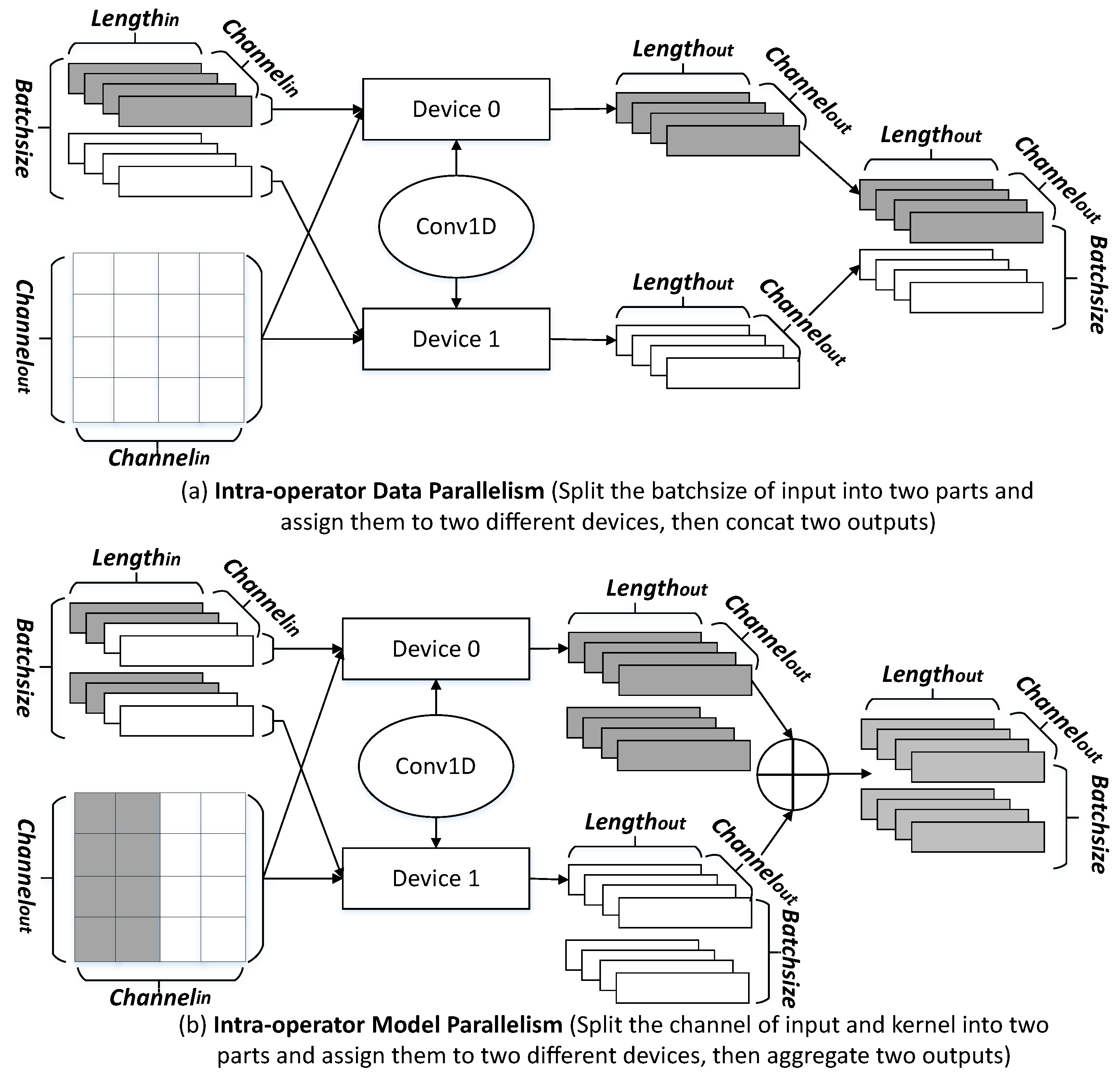
Computationally intensive operators will affect the end-to-end execution performance of the model because of their high computational costs. In this section, for the computationally intensive operators in DNNs, we adopt intra-operator parallelism based on tensor dimensions. Firstly, the specified axis of the input of computationally intensive operators is partitioned. Then, these partitions are assigned to different devices to compute disjoint subsets of the original operator’s output tensors. According to the different partition specifications of tensor dimensions, operator parallelism can be classified as data parallelism or model parallelism.
Taking Conv1D as an example, Figure 2a shows the data parallelism for the convolution operator. The input is assigned to two devices by splitting the axis of the batch size. Each device executes Conv1D using the entire convolution kernel tensor and one of the sub-matrices to calculate the output tensor of the corresponding batch. The result of the original operator is collected from the outputs on the two devices. Figure 2b shows the model parallelism for the convolution operator. The input and convolution kernel are assigned to two devices by splitting the axis of the channel. Each device executes Conv1D using part of the convolution kernel tensor and one of the sub-matrices to calculate the output tensor of the corresponding channel. The result of the original operator is also gathered from the outputs on the two devices.

4.2. Generation of Dynamic Critical Path

Intra-operator parallelism makes the graph search space more complex than inter-operator parallelism. Simultaneously, as operators are dynamically scheduled to be executed on different devices, the available devices of the cluster will change dynamically. In a DAG, the critical path is the path with the most expensive cost from the entry node to the exit node, which determines the maximum end-to-end execution time of the computational graph. The dynamic environment will lead to changes in the critical path of the computational graph, which affects the end-to-end execution time of the computational graph. For the DAG graph, this paper adaptively generates critical paths based on the dynamic scenarios and guides the placement of nodes in the device.
To implement the above method, we introduce the concepts of the earliest start time (EST), latest start time (LST), critical node (CN), critical path (CP), and node priority (NP) based on [20]. Their definitions are as follows:
Definition 8
(Earliest Start Time). The earliest start time (EST) of node o i on device v k is the earliest time when o i can start the execution in the entire computational graph. It can be defined as Formula (6):
E S T ( o i , v k ) = max o j p r e d ( o i ) { E S T ( o j , v l ) + E T ( o j , v l ) + w ( o i k , o j l ) }
where E T ( o j , v l ) represents the execution time of node o j on device v l and w ( o i k , o j l ) represents the communication cost between o i on v k and o j on v l . The EST of the entry node E S T ( o e n t r y , v 1 ) = 0 . According to Formula (6), the EST can be calculated by traversing the computational graph in a breadth-first search method starting from o e n t r y .
Definition 9
(Latest Start Time). The latest start time (LST) of node o i on device v k is the latest time when o i can start execution without delaying the execution of the entire computational graph. It can be defined as Formula (7):
L S T ( o i , v k ) = min o j s u c c ( o i ) { L S T ( o j , v l ) E T ( o j , v l ) w ( o i k , o j l ) }
where the latest start time of the exit node L S T ( o e x i t , v e ) is the total time for the execution of the critical path. Similar to the calculation of the EST, the LST can also be calculated by traversing the inverse computational graph in a breadth-first search method.
Definition 10
(Critical Node). The node on the critical path is the critical node. In the DAG, if the EST and LST of node o i on device v k satisfy E S T ( o i , v k ) = L S T ( o i , v k ) , node o i is a critical node:
C N ( o i ) = t r u e , i f E S T ( o i , v k ) = L S T ( o i , v k ) f a l s e , o t h e r w i s e
Definition 11
(Critical Path). Define the path from the entry node o e n t r y to the exit node o e x i t in the DAG that satisfies the maximum cost (the computational cost and the communication cost) as the critical path (CP).
Definition 12
(Node Priority). Node priority refers to the importance of a node during scheduling. The smaller the difference between the EST and LST of a node is, the greater the impact is on the end-to-end execution time of the critical path and the greater the priority of the node is. The node priority of o i is expressed by Formula (9):
S c o r e ( o i ) = 1 / ( L S T ( o i , v k ) E S T ( o i , v k ) + e p s )
where S c o r e ( o i ) represents the node priority of o i , e p s represents a non-zero constant value, it prevents an exception from occurring when L S T ( o i , v k ) E S T ( o i , v k ) = 0 .
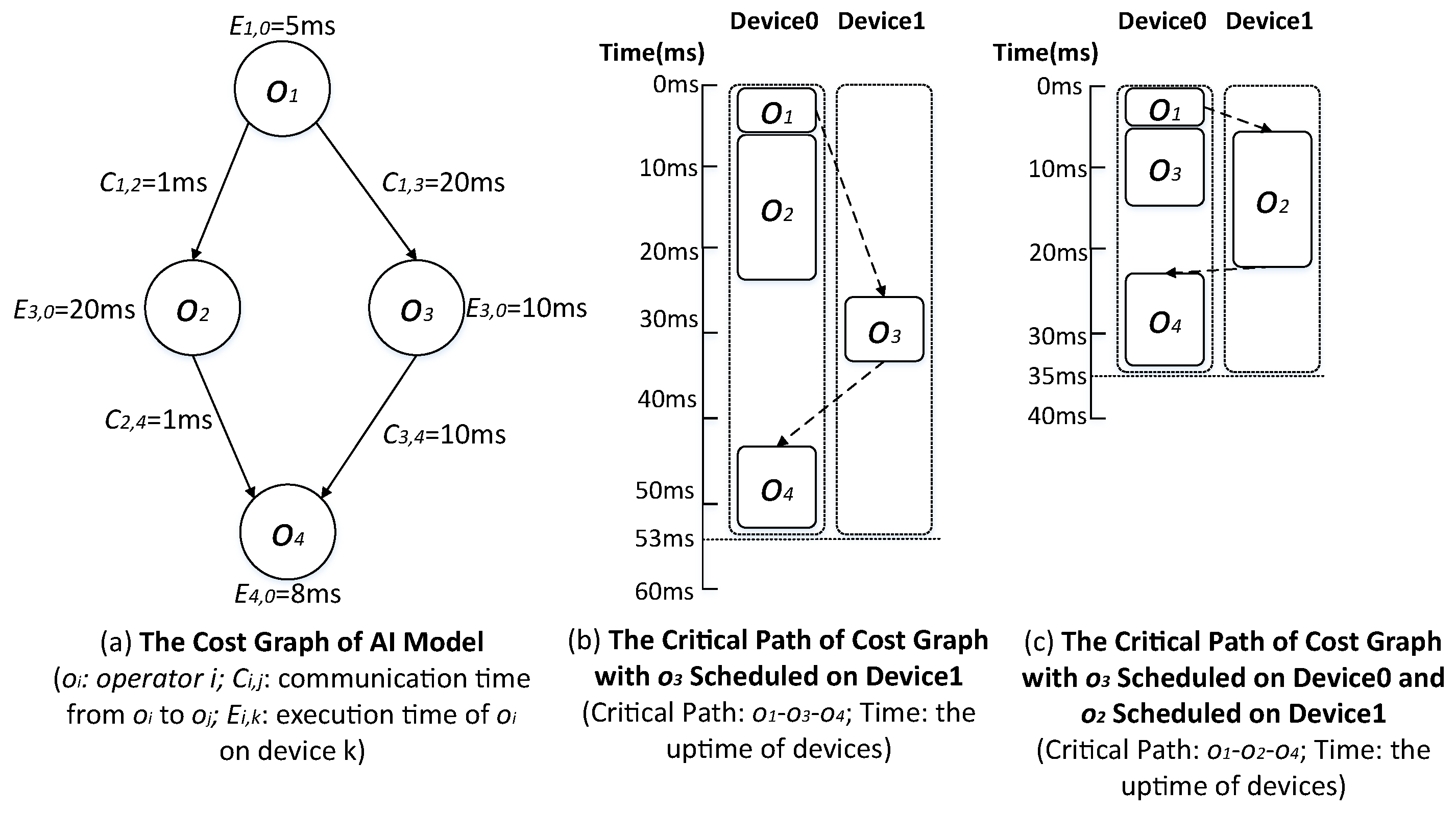
According to the above definition, the critical path determines the longest end-to-end execution time of the computational graph. Actually, in the progress of the schedule, the available resources of the device cluster change dynamically. This leads to changes in the execution performance of nodes on different devices. Moreover, this also leads to dynamic changes in the critical nodes and critical paths. For example, as shown in Figure 3a, o 2 and o 3 have no dependencies during execution, so they can be executed in parallel. As shown in Figure 3b, if o 2 is scheduled on Device0 for execution and o 3 is scheduled on Device1 for execution, the critical path of the DAG is o 1 - o 3 - o 4 and the critical path length is 53. As shown in Figure 3c, if o 3 is scheduled on Device0 for execution and o 2 is scheduled on Device1 for execution, the critical path of the DAG becomes o 1 - o 2 - o 4 and the critical path length becomes 35. Obviously, the strategy in Figure 3c is more optimal. Since operators are scheduled on different devices, the critical path of the computational graph will change. Therefore, the main goal of the dynamic critical path generation is to find the optimal scheduling strategy.
As shown in Figure 3, different operator scheduling strategies affect the selection of devices in the scheduling process, which will lead to changes in critical nodes and critical paths. In this paper, we call the critical path that changes with the dynamic scenarios the dynamic critical path (DCP).
The above analysis shows that the critical path length of the computational graph is an important indicator for the scheduling of the operators. It represents the end-to-end execution time of the computational graph. Therefore, we define the dynamic critical path length (DCPL) as follows:
D C P L = max o i O , v k V { E S T ( o i , v k ) + E T ( o i , v k ) }
where E S T ( o i , v k ) represents the EST of node o i on device v k and E T ( o i , v k ) represents the execution time of node o i on device v k .
Since DCPL is the maximum value of the earliest finish time (e.g., E S T ( o i , v k ) + E T ( o i , v k ) ) of all paths, it can be used to determine the upper limit of the node start time. Therefore, in the dynamic priority scheduling process, the EST and LST can be generated through DCPL dynamically if a schedulable node is not assigned.
To determine the dynamic critical nodes (DCN) on the dynamic critical path (DCP), we assume that the DCP ranges from the entry node o e n t r y to the exit node o e x i t . The specific method is as follows:
  • For all nodes in the computational graph, calculate the corresponding EST and LST.
  • According to Formula (8), determine the critical nodes. If node o i satisfies E S T ( o i , v k ) = L S T ( o i , v k ) , it can be marked as a critical node.
  • According to the identified critical nodes and the node dependencies in the computational graph, use the breadth-first search method to generate the DCP.

4.3. Optimal Scheduling Based on Operator Priority

According to Section 4.2, the DCP determines the longest end-to-end execution time of the entire computational graph in dynamic scenarios. In this section, we propose a critical path optimal scheduling method based on node priority, which can optimize the end-to-end longest execution time of the computational graph.
The key to this method is to schedule nodes with high priority, which ensures that nodes with a small time-optimizable execution range are finished at the earliest time. The critical nodes satisfy E S T = L S T and S c o r e = 1 / e p s , which have the highest priority. Therefore, the marked critical nodes can be scheduled preferentially to reduce the cost of computing the node priority.
The specific method to implement the optimal scheduling of critical paths according to the node priority is as follows:
(1). Find the marked critical nodes from the schedulable nodes based on the priority scheduling of critical nodes.
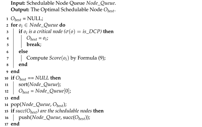
If all the parent nodes of a node o i have been scheduled to the device, but o i has not been scheduled and o i is a schedulable node, the selection of the optimal schedulable node is as follows: First of all, the marked critical nodes among the schedulable nodes will be scheduled preferentially. Then, if there is no marked critical node in the schedulable nodes, calculate the node priority of all nodes using Formula (9). Sort the schedulable nodes by node priority from largest to smallest. The first node (which has the highest priority) from the sequence is the optimal schedulable node. The specific details are shown in Algorithm 1:
Algorithm 1: The algorithm for finding the optimal schedulable node (Sort_Node ( N o d e _ Q u e u e ) )
Mathematics 10 04788 i001
(2). Find the matching device for the optimal schedulable node.
For the optimal schedulable node, we adopt the following method to find the matching device.
Firstly, according to the node (operator) resource requirements (e.g., communication, computation, and memory) and the idle resources of the device, we select the device set that satisfies the resource requirements for the nodes (operators).
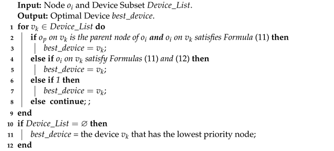
Then, assuming that the total number of nodes in the graph search space is n, we select devices that satisfy resource requirements for schedulable node o i ( i = 1 , 2 , , n ); where the devices need to satisfy the execution time requirement of node o i , the scheduling process cannot affect the execution of scheduled nodes on these devices. For a device v k that satisfies the resource requirements of node o i , suppose that o j ( j = 1 , 2 , , n 1 ) and o m ( m = 1 , 2 , , n 1 ) are the scheduled nodes on this device. If o i will be scheduled to device v k , the execution order of o j , o i , and o m on device v k is o j o i o m . Suppose that o p ( p = 1 , 2 , , i 1 ) represents a parent node of o i in the computational graph. Then, we adopt Formula (11) to determine whether node o i can be scheduled to device v k :
E T ( o i , v k ) min { L S T ( o i , v k ) + E T ( o i , v k ) , L S T ( o m , v k ) } max { E S T ( o i , v k ) , E S T ( o j , v k ) + E T ( o j , v k ) } i f t h e p a r e n t n o d e o p o f o i i s n o t s c h e d u l e d t o v k . E T ( o i , v k ) min { L S T ( o i , v k ) + E T ( o i , v k ) , L S T ( o m , v k ) } max { E S T ( o i , v k ) , E S T ( o j , v k ) + E T ( o j , v k ) } i f t h e p a r e n t n o d e o p o f o i i s s c h e d u l e d t o v k .
When o p is not scheduled to v k , if the execution time of o i on v k is less than the difference between the latest start time of o m on v k ( L S T ( o m , v k ) ) and the earliest finish time of o j on v k ( E S T ( o j , v k ) + E T ( o j , v k ) ), then node o i can be scheduled between o j and o m on v k . When o p is a scheduled node on v k , the communication cost between o p and o i on v k is 0 if o i is scheduled to o i . However, the EST (calculated by Formula (6)) and LST (calculated by Formula (7)) of o i on v k include the ( o i l , o p k ) between o i on v l and o p on v k . Therefore, it is necessary to recalculate the earliest start time E S T ( o i , v k ) and the latest start time L S T ( o i , v k ) of o i when o i and o p are scheduled to the same device v k , where E S T ( o i , v k ) = E S T ( o i , v k ) w ( o i l , o p k ) and L S T ( o i , v k ) = L S T ( o i , v k ) w ( o i l , o p k ) . If the execution time of o i on v k is less than the difference between the latest start time of o m on v k ( L S T ( o m , v k ) ) and the earliest finish time of o j on v k ( E S T ( o j , v k ) + E T ( o j , v k ) ), then node o i can be scheduled between o j and o m on v k . For node o i , there may be multiple devices that satisfy Formula (11). We can record all satisfied devices with a device subset.
Lastly, we find the optimal device from the selected device subset. (1) If node o i and its parent node o p can be scheduled to the same device v p , select v p preferentially as the optimal device of node o i to reduce the communication cost. (2) If node o i and its leaf node o c can be scheduled to the same device v b , select v b preferentially as the optimal device of node o i , where o c needs to be selected based on the node priority and v b needs to be selected based on the execution time of the node o c on the device. The selection of the optimal device v b and the optimal child node o c is shown in Formula (12):
o c arg max o k s u c c ( o i ) { S c o r e ( o k ) } v b arg max v k V { E T ( o c , v k ) + E T ( o i , v k ) }
where o c has the highest node priority in the leaf node set of o i . V presents the new device subset which satisfies the scheduling of o i and o c in the original device subset. v b is the device that minimizes the execution time of o i and o c ( E T ( o c , v k ) + E T ( o i , v k ) ).
(3) We select the device v k from the device subset that satisfies the earliest execution of o i as the optimal device. v k can execute o i as soon as possible. (4) When no device satisfies the above conditions, according to the node priority, select the device that executes the lowest priority node as the optimal device of node o i .
The specific details are shown in Algorithm 2.
Algorithm 2: Algorithm of finding optimal device (Find_Slot( o i , D e v i c e _ L i s t ))
Mathematics 10 04788 i002
(3). Update the graph search space according to the scheduling.
After the node scheduling is finished, update the graph search space according to the scheduling situation. The updated content mainly includes the weight of the edge, the EST and LST of the scheduled node o i , and the EST and LST of the unscheduled node. The specific update method is as follows.
Firstly, when the scheduled node o i is scheduled to the device where the parent node o p is located, the communication cost of edge from o p to o i ( w ( o i k , o p k ) ) is set to 0. Then, according to the scheduling of the scheduled node o i on the device, update the EST and LST of o i . Finally, iteratively update the EST and LST of all unscheduled nodes through Formulas (6) and (7) after the update of the graph search space.
After the graph search space update, perform a new round of node optimization scheduling, and repeat this process until the optimal parallel strategy is found.
4.4. Algorithm Implementation

The specific implementation of FD-DPS is shown in Algorithm 3:
Lines 2–6 implement the intra-operator parallelism, which split the operators with the tensor dimension according to the operator attributes. Lines 9–14 implement the generation of dynamic critical paths, which calculate the EST and LST of all nodes and determine all DCP nodes for subsequent scheduling. Lines 15–26 implement optimal scheduling. Among them, line 15 calls the finding optimal node algorithm (Sort_Node( N o d e _ Q u e u e )) to find the optimal schedulable node, and line 24 calls the finding optimal device algorithm (Find_Slot( o i , D e v i c e _ L i s t )) to find the optimal device for the optimal schedulable node.
The FD-DPS algorithm returns the optimal parallel strategy S and optimal sequence queue Q of all nodes in the DAG. The main time cost of Algorithm 3 comes from sorting the nodes according to node priority and finding the most appropriate device for the schedulable node.
Algorithm 3: FD-DPS: The Algorithm for Dynamic Critical Path Generation Based on DAG
Mathematics 10 04788 i003

5. Experiment

To verify the effectiveness and performance of FD-DPS, we conducted experiments on Vgg_16, InceptionV3, and other models, and compare the results with those from FastT and MP-DPS. Specifically, we compare them in terms of single-round iteration time, intra-operator parallelism performance, strategy search time, and dynamic search time.

5.1. Experimental Setup

(1) System Model.
We selected six widely used DNNs to evaluate the effectiveness of FD-DPS, as shown in Table 3.
These DNNs have different numbers of operators and edges in the computational graphs so that we can evaluate the scalability and performance of FD-DPS at different scales.
(2) Baseline.
We chose three deep learning training strategies as baselines.
Data Parallelism: Data parallelism is suitable for scenarios where the memory capacity of the devices cannot hold all the training data. It divides the data through certain division methods (e.g., data sample division and data dimension division) and stores the data in different devices. After that, each device uses local data to update the model in an optimized way. The experiment in this paper adopts simple data division based on TensorFlow slim [33].
FastT: Based on the data flow graph of TensorFlow, we propose a white-box algorithm to compute strategies that consume few computing resources in a short time. The white-box algorithm is used to automatically identify the optimal parallel strategies in DNNs to speed up model training. Compared with reinforcement learning, the strategy search time of FastT is relatively short. However, FastT does not consider the dynamic memory ratio during model training, so there is still room for optimization of this scheduling algorithm.
MP-DPS: MP-DPS uses computational graphs in the form of data flow graphs. It optimizes operator placement through the DAG scheduling algorithm. Firstly, MP-DPS constructs a graph search space by extracting the features of the original computational graph and device topology. Then, it reduces the search space by merging nodes with computing power awareness. Finally, it implements optimal scheduling by predicting the path cost in DAG to find the optimal parallel strategy. However, the dynamic changes of the scenarios will lead to the problem that static methods are difficult to search for the optimal distributed parallel strategy, so MP-DPS still has room for optimization in strategy search time and performance.
(3) Software and Hardware Environment:
The experimental hardware environment of this paper is a single server, including a Genuine Intel CPU and eight NVIDIA Tesla P100 GPUs. The specific software environment is shown in Table 4.

5.2. Strategy Execution Performance

In this section, we use the single-round iteration performance of the generation strategy as the measurement index and compare FD-DPS, MP-DPS, and FastT. The comparison results are shown in Table 5.
Compared with MP-DPS and FastT, FD-DPS performs better when the model size increases and the number of devices increases. When four GPUs are used, FD-DPS significantly exceeds FastT and MP-DPS. Its single-round iteration performance on ResNet_50 and PnasNet_mobile shows an 18.11% and 10.54% improvement over FastT and MP-DPS, respectively. When eight GPUs are used, FD-DPS more significantly exceeds FastT and MP-DPS, with speed increases in the single-round iteration performance of 23.83% and 12.76%, respectively, on PnasNet_mobile. This is because FD-DPS calculates the scheduling priority several times during its policy search based on global resources, whereas the FastT and MP-DPS methods do not consider dynamic resources. The FastT method uses static operator priority according to the critical path, and MP-DPS uses node merging and path prediction to search for the distributed strategy. Thus, the FD-DPS method can find a better scheduling policy than the above methods.
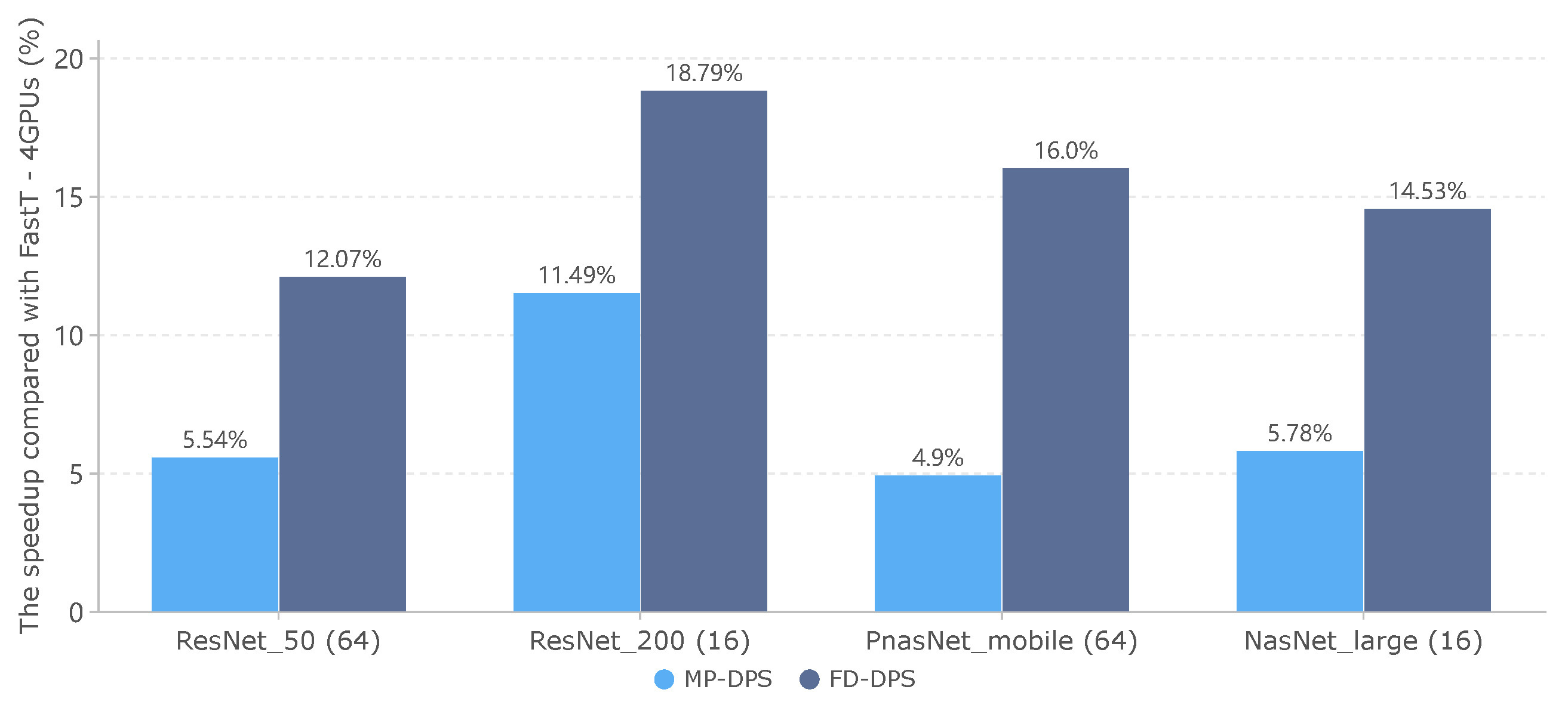
To simulate the inter-operator communication environment, we test the cross-container communication and scheduling on a single server. We deployed two dockers (each with four GPUs) on the same server and included the communication time between dockers in the overall performance cost.
As shown in Figure 4, after incorporating the communication cost between devices, FD-DPS also achieves a greater effect in the single-round iteration performance compared with MP-DPS. Specifically, on PnasNet_mobile, the single-round iteration performance of MP-DPS compared with FastT was only improved by 4.9%. However, the single-round iteration performance of FD-DPS compared with FastT was improved by 16.0%, which was 11.1% better than that of MP-DPS.

5.3. Intra-Operator Parallelism Performance

In this section, we conduct experiments to evaluate the intra-operator parallelism performance of FD-DPS, compared to D-DPS(-F) and MD-DPS.
Table 6 shows the splitting decisions, the execution time (before splitting), and parameter sizes of some representative operators in Vgg_16. Since the convolution (e.g., Conv1_1, Conv1_2, and Conv1_2bp) operator is a computationally intensive operator. Its execution time is longer than other operators, and it is easiest to be split with the tensor dimension. The fully connected (e.g., Fc6) operator that contains many parameters is a parameter-intensive operator. For the FD-DPS algorithm with operator segmentation based on the tensor dimension, the fully connected operator is not easy to split.
Therefore, when verifying the intra-operator parallelism performance of FD-DPS, it is necessary to select models with more convolution operators for comparative experiments.
As shown in Table 7, compared with the D-DPS(-F) algorithm without intra-operator parallelism, the performance of FD-DPS has been greatly improved in the use case of four GPUs. Among them, FD-DPS has the best effect on NasNat_large, achieving a speedup of 13.87% compared with D-DPS(-F). The experiment also shows that the use of intra-operator parallelism further refines the granularity of the operator, the larger search space, and more flexible strategy search. After intra-operator parallelism, FD-DPS can find the suboptimal or optimal parallel strategy.

5.4. Strategy Search Performance

To analyze the impact of dynamic scheduling on the parallel strategy search time, this section conducts comparative experiments on MP-DPS, D-DPS(-F), and FD-DPS under the eight GPUs configuration.
As shown in Figure 5, FD-DPS has a relatively longer parallel strategy search time than FastT, when the trained model is small. However, the parallel strategy search time of the FD-DPS is much less than that of FastT when the trained model is large. The experimental results show that FD-DPS is better than FastT in the performance of automatic parallel strategy searches for large-scale models. Particularly, on PnasNet_mobile, the automatic parallel strategy search time of FD-DPS is reduced by 185.8s compared with FastT. The experimental results demonstrate that FD-DPS has better scalability and robustness than FastT when dealing with large-scale models.
MP-DPS has the least search cost among the three algorithms. Particularly, on NasNet_large model, MP-DPS reduces the dynamic search time by 95.5 s (compared with D-DPS(-F)) and 117.3 s (compared with FD-DPS), respectively. Simultaneously, we can notice that D-DPS(-F) reduces the parallel strategy search time by 21.8 s compared with FD-DPS. Therefore, the improvement of single-round iteration performance is produced under the premise of increasing the search cost.
However, compared with the increase in search cost, the performance improvement of FD-DPS brings more benefits. Assuming that NasNet_large is trained on eight GPUs, MP-DPS is 117.3 s less than FD-DPS in dynamic search time. As shown in Table 5, the cost of FD-DPS under the single-round iteration is 0.619 s less than that of MP-DPS. Under the premise that the batch size is 16 and the dataset is 10,000 images, it takes 625 iterations to train CIFAR-10 to complete one epoch. Additionally, the time saved by training one epoch in distributed parallel is 386.878 s, which is enough to offset the increase in time consumption caused by parallel strategy optimization. The parallel performance gains brought by FD-DPS are greater when training large-scale DNNs for multiple rounds of iteration.
As results of Table 4 and Figure 5 show, for FD-DPS, there was a small increase in search time because using intra-operator parallelism compared with D-DPS (F) and MP-DPS. However, the single-round iteration performance of FD-DPS has been greatly improved compared with D-DPS (F) and MP-DPS.

6. Conclusions

To address the problem of the low efficiency of the static auto-parallel method based on graph algorithms caused by complex model structures and dynamic changes in the execution environment, this paper proposes an adaptive distributed parallel training method based on the dynamic generation of critical paths for DAG called FD-DPS. The proposed method reduces the problem of finding an optimal distributed parallel policy to the problem of finding an optimal path in a directed graph. It searches for the optimal path with intra-operator parallelism with tensor dimension and dynamical critical paths of DAG, which can expand the searching space and deal with the effect of a dynamic environment on model execution performance. The experimental results show that compared with FastT and MP-DPS, FD-DPS can effectively optimize the node placement and scheduling sequence. It also can reduce the iteration time of the models and optimize the training performance.
Although FD-DPS utilizes an automatically distributed parallel method to achieve inter-operator parallelism, intra-operator parallelism with a tensor dimension is based on expert experience. This will increase the workload of the designer and result in a suboptimal intra-operator parallelism strategy. Therefore, our future work will focus on the implementation of automatic intra-operator parallelism to improve the FD-DPS method. By implementing an automatically distributed parallel method for both inter-operator and intra-operator parallelism, we will update the FD-DPS method and apply it to accelerating model training.

Author Contributions

Conceptualization, J.Z. and Y.R.; methodology, Y.Z.; supervision, Y.Z.; project administration, Y.Z.; software, W.W. and Y.D.; data curation, Y.Z. and G.Y. All authors have read and agreed to the published version of the manuscript.

Funding

This research was funded by the National Natural Science Foundation of China under Grant (62072146, 61972358); the Key Research and Development Program of Zhejiang Province under Grant No.2021C03187; and the State Key Laboratory of Computer Architecture (ICT, CAS) under Grant No. CARCHB202120.

Institutional Review Board Statement

Not applicable.

Informed Consent Statement

Not applicable.

Data Availability Statement

Not applicable.

Conflicts of Interest

The authors declare no conflict of interest.

Abbreviations

The following abbreviations are used in this manuscript:
DAGdirected acyclic graph
DFTdensity functional theory
DNNdeep neural network
ANNartificial neural network
RMSroot-mean-square
LSTMlong short-term memory
MLmachine learning
ESTearliest start time
LSTlatest start time
CNcritical node
CPcritical path
NPnode priority
ETexecution time
DCPdynamic critical path
DCPLdynamic critical path length
DCNdynamic critical node
DPdata parallel

References

  1. Thompson, A.P.; Aktulga, H.M.; Berger, R.; Bolintineanu, D.S.; Brown, W.M.; Crozier, P.S.; In’t Veld, P.J.; Kohlmeyer, A.; Moore, S.G.; Nguyen, T.D.; et al. LAMMPS-a flexible simulation tool for particle-based materials modeling at the atomic, meso, and continuum scales. Comput. Phys. Commun. 2022, 271, 108171. [Google Scholar] [CrossRef]
  2. Schmidt, J.; Marques, M.R.; Botti, S.; Marques, M.A. Recent advances and applications of machine learning in solid-state materials science. NPJ Comput. Mater. 2019, 5, 1–36. [Google Scholar] [CrossRef] [Green Version]
  3. Lu, D.; Wang, H.; Chen, M.; Lin, L.; Car, R.; Weinan, E.; Jia, W.; Zhang, L. 86 PFLOPS Deep Potential Molecular Dynamics simulation of 100 million atoms with ab initio accuracy. Comput. Phys. Commun. 2021, 259, 107624. [Google Scholar] [CrossRef]
  4. Jumper, J.; Evans, R.; Pritzel, A.; Green, T.; Figurnov, M.; Ronneberger, O.; Tunyasuvunakool, K.; Bates, R.; Žídek, A.; Potapenko, A.; et al. Highly accurate protein structure prediction with AlphaFold. Nature 2021, 596, 583–589. [Google Scholar] [CrossRef] [PubMed]
  5. Burger, L.; Van Nimwegen, E. Disentangling direct from indirect co-evolution of residues in protein alignments. PLoS Comput. Biol. 2010, 6, e1000633. [Google Scholar] [CrossRef] [PubMed]
  6. Lin, Z.; Akin, H.; Rao, R.; Hie, B.; Zhu, Z.; Lu, W.; dos Santos Costa, A.; Fazel-Zarandi, M.; Sercu, T.; Candido, S.; et al. Language models of protein sequences at the scale of evolution enable accurate structure prediction. bioRxiv 2022. [Google Scholar] [CrossRef]
  7. Brown, T.; Mann, B.; Ryder, N.; Subbiah, M.; Kaplan, J.D.; Dhariwal, P.; Neelakantan, A.; Shyam, P.; Sastry, G.; Askell, A.; et al. Language models are few-shot learners. Adv. Neural Inf. Process. Syst. 2020, 33, 1877–1901. [Google Scholar]
  8. Wu, Y.; Schuster, M.; Chen, Z.; Le, Q.V.; Norouzi, M.; Macherey, W.; Krikun, M.; Cao, Y.; Gao, Q.; Macherey, K.; et al. Google’s neural machine translation system: Bridging the gap between human and machine translation. arXiv 2016, arXiv:1609.08144. [Google Scholar]
  9. Sutskever, I.; Vinyals, O.; Le, Q.V. Sequence to sequence learning with neural networks. Adv. Neural Inf. Process. Syst. 2014, 27, 3104–3112. [Google Scholar]
  10. Sun, S.; Chen, W.; Bian, J.; Liu, X.; Liu, T.Y. Slim-DP: A multi-agent system for communication-efficient distributed deep learning. In Proceedings of the 17th International Conference on Autonomous Agents and MultiAgent Systems, Stockholm, Sweden, 10–15 July 2018; pp. 721–729. [Google Scholar]
  11. Barnard, S.T.; Simon, H.D. Fast multilevel implementation of recursive spectral bisection for partitioning unstructured problems. Concurr. Pract. Exp. 1994, 6, 101–117. [Google Scholar] [CrossRef]
  12. Addanki, R.; Venkatakrishnan, S.B.; Gupta, S.; Mao, H.; Alizadeh, M. Placeto: Learning generalizable device placement algorithms for distributed machine learning. arXiv 2019, arXiv:1906.08879. [Google Scholar]
  13. Liu, J.; Wu, Z.; Yu, D.; Ma, Y.; Feng, D.; Zhang, M.; Wu, X.; Yao, X.; Dou, D. Heterps: Distributed deep learning with reinforcement learning based scheduling in heterogeneous environments. arXiv 2021, arXiv:2111.10635. [Google Scholar]
  14. Chen, Z. RIFLING: A reinforcement learning-based GPU scheduler for deep learning research and development platforms. Softw. Pract. Exp. 2022, 52, 1319–1336. [Google Scholar] [CrossRef]
  15. Cai, Z.; Yan, X.; Ma, K.; Wu, Y.; Huang, Y.; Cheng, J.; Su, T.; Yu, F. Tensoropt: Exploring the tradeoffs in distributed dnn training with auto-parallelism. IEEE Trans. Parallel Distrib. Syst. 2021, 33, 1967–1981. [Google Scholar] [CrossRef]
  16. Zheng, L.; Li, Z.; Zhang, H.; Zhuang, Y.; Chen, Z.; Huang, Y.; Wang, Y.; Xu, Y.; Zhuo, D.; Gonzalez, J.E.; et al. Alpa: Automating Inter-and Intra-Operator Parallelism for Distributed Deep Learning. arXiv 2022, arXiv:2201.12023. [Google Scholar]
  17. Unger, C.; Jia, Z.; Wu, W.; Lin, S.; Baines, M.; Narvaez, C.E.Q.; Ramakrishnaiah, V.; Prajapati, N.; McCormick, P.; Mohd-Yusof, J.; et al. Unity: Accelerating {DNN} Training Through Joint Optimization of Algebraic Transformations and Parallelization. In Proceedings of the 16th USENIX Symposium on Operating Systems Design and Implementation (OSDI 22), Carlsbad, CA, USA, 11–13 July 2022; pp. 267–284. [Google Scholar]
  18. Jia, Z.; Lin, S.; Qi, C.R.; Aiken, A. Exploring Hidden Dimensions in Parallelizing Convolutional Neural Networks. In Proceedings of the ICML, Stockholm, Sweden, 10–15 July 2018; pp. 2279–2288. [Google Scholar]
  19. Wang, M.; Huang, C.C.; Li, J. Supporting very large models using automatic dataflow graph partitioning. In Proceedings of the Fourteenth EuroSys Conference 2019, Dresden, Germany, 25–28 March 2019; pp. 1–17. [Google Scholar]
  20. Yi, X.; Luo, Z.; Meng, C.; Wang, M.; Long, G.; Wu, C.; Yang, J.; Lin, W. Fast training of deep learning models over multiple gpus. In Proceedings of the 21st International Middleware Conference, Delft, The Netherlands, 7–11 December 2020; pp. 105–118. [Google Scholar]
  21. Zeng, Y.; Ding, Y.; Ou, D.; Zhang, J.; Ren, Y.; Zhang, Y. MP-DPS: Adaptive Distributed Training for Deep Learning Based on Node Merging and Path Prediction; CCF Transactions on High Performance Computing: Beijing, China, 2022; pp. 1–13. [Google Scholar]
  22. Stevens, R.; Taylor, V.; Nichols, J.; Maccabe, A.B.; Yelick, K.; Brown, D. AI for Science: Report on the Department of Energy (DOE) Town Halls on Artificial Intelligence (AI) for Science; Technical Report; Argonne National Lab. (ANL): Argonne, IL, USA, 2020.
  23. Collins, W.; Tissot, P. An artificial neural network model to predict thunderstorms within 400 km2 South Texas domains. Meteorol. Appl. 2015, 22, 650–665. [Google Scholar] [CrossRef]
  24. Negoita, G.A.; Vary, J.P.; Luecke, G.R.; Maris, P.; Shirokov, A.M.; Shin, I.J.; Kim, Y.; Ng, E.G.; Yang, C.; Lockner, M.; et al. Deep learning: Extrapolation tool for ab initio nuclear theory. Phys. Rev. C 2019, 99, 054308. [Google Scholar] [CrossRef] [Green Version]
  25. Armstrong, D.J.; Gamper, J.; Damoulas, T. Exoplanet validation with machine learning: 50 new validated Kepler planets. Mon. Not. R. Astron. Soc. 2021, 504, 5327–5344. [Google Scholar] [CrossRef]
  26. Chan, M.C.; Stott, J.P. Deep-CEE I: Fishing for galaxy clusters with deep neural nets. Mon. Not. R. Astron. Soc. 2019, 490, 5770–5787. [Google Scholar] [CrossRef]
  27. Zhang, H.; Li, Y.; Deng, Z.; Liang, X.; Carin, L.; Xing, E. Autosync: Learning to synchronize for data-parallel distributed deep learning. Adv. Neural Inf. Process. Syst. 2020, 33, 906–917. [Google Scholar]
  28. Chen, M.; Beutel, A.; Covington, P.; Jain, S.; Belletti, F.; Chi, E.H. Top-k off-policy correction for a REINFORCE recommender system. In Proceedings of the Twelfth ACM International Conference on Web Search and Data Mining, Melbourne, VIC, Australia, 11–15 February 2019; pp. 456–464. [Google Scholar]
  29. Jia, Z.; Zaharia, M.; Aiken, A. Beyond Data and Model Parallelism for Deep Neural Networks. Proc. Mach. Learn. Syst. 2019, 1, 1–13. [Google Scholar]
  30. Abdullahi, M.; Ngadi, M.A. Hybrid symbiotic organisms search optimization algorithm for scheduling of tasks on cloud computing environment. PLoS ONE 2016, 11, e0158229. [Google Scholar]
  31. Li, F.; Xu, Z.; Li, H. A multi-agent based cooperative approach to decentralized multi-project scheduling and resource allocation. Comput. Ind. Eng. 2021, 151, 106961. [Google Scholar] [CrossRef]
  32. Jeon, B.; Cai, L.; Srivastava, P.; Jiang, J.; Ke, X.; Meng, Y.; Xie, C.; Gupta, I. Baechi: Fast device placement of machine learning graphs. In Proceedings of the 11th ACM Symposium on Cloud Computing, Virtual Event, USA, 19–21 October 2020; pp. 416–430. [Google Scholar]
  33. Silberman, N. TF-Slim: A Lightweight Library for Defining, Training and Evaluating Complex Models in TensorFlow. 2017. Available online: https://github.com/google-research/tf-slim (accessed on 15 December 2022).
Figure 1. Architecture of FD-DPS Method.
Mathematics 10 04788 g001
Figure 2. Schematic Diagram of intra-operator parallelism.
Mathematics 10 04788 g002
Figure 3. Critical Path Diagram.
Mathematics 10 04788 g003
Figure 4. Single-round iteration time speedup comparison (two dockers with eight GPUs).
Mathematics 10 04788 g004
Figure 5. The optimal strategy search time comparison of FD-DPS and baselines.
Mathematics 10 04788 g005
Table 1. Typical AI Models for Science.
ModelFieldContribution
TANN [23]Atmospheric scienceForecast the likelihood of thunder-storms in a region several hours in advance.
ANN [24]PhysicsObtain the ground-state energy and the ground-state point-proton RMS radius along with their extrapolation uncertainties.
VESPA [25]AstronomyValidate 50 Keplerian plane.
Deep-CEE [26]AstronomySearch for galaxy clusters without photometric catalog.
DeePMD-kit [3]Molecular dynamicsDrive large-scale molecular dynamics simulation with ab initio accuracy.
AlphaFold [4]BioinformaticsPredict protein structure.
Table 2. Distributed Parallel Methods.
MethodWorkContribution
Distributed parallel method based on expert experienceGNMT [8], Seq2Seq [9]Place the LSTM, Attention, and SoftMax on different devices.
Slim-DP [10]Random partition based on backbone network exploration.
RSB [11]Matrix multiplication inside the operator.
Automatically distributed parallel methodAutoSync [27]Employ machine learning to find the distributed strategy.
REINFORCE [28]Update the distributed strategy by real execution time.
Placeto [12]Placeto generalizes distributed strategy by capturing model structure with reinforcement.
FlexFlow [29]Build a performance evaluation model to guide the optimal parallel strategy search in dynamic programming.
OptCNN [18]Build a performance evaluation model to guide the optimal parallel strategy search in dynamic programming.
Tofu [19]Adopt recursive segmentation and graph coarsening based on OptCNN.
FastT [20]Adopt fine-grained operator priority and the critical path to place and schedule operators.
MP-DPS [21]Find the distributed strategy based on node merging and path prediction.
Alpa [16]Apply integer linear programming to intra-operator parallelism and dynamic programming to inter-operator parallelism.
Table 3. Deep neural network model and corresponding dataset.
SourceDNNs (Batch)Number of OperatorsNumber of EdgesDataset
TF-SlimVgg_16 (64)39325461CIFAR-10
InceptionV3 (64)12,74521,928
ResNet_50 (64)12,69224,345
ResNet_200 (16)45,47282,347
PnasNet_mobile (64)62,19291,957
NasNet_large (16)83,206148,548
Table 4. Experimental software environment.
Environment NameEnvironment Version
SystemUbuntu 16.04.4 LTS
KernelLinux 4.15.0-123-generic
GPU DriverNVIDIA-418.87.00
CUDACUDA 10.0.130
TensorFlowTensorFlow 1.14.0
PythonPython 3.7.10
Table 5. Single-round iteration time comparison of FD-DPS and baseline.
Model (batch)Single-GPU (s)Multi-GPUsDP (s)FastT (s)MP-DPS (s)Speedup 1FD-DPS (s)Speedup 2
Vgg_16 (64)0.79421.2721.1221.0661.41%1.0516.33%
41.7701.9751.9054.88%1.8128.25%
InceptionV3 (64)0.57420.7380.7120.7022.42%0.6853.79%
40.9430.9120.8725.62%0.8239.76%
ResNet_50 (64)0.39440.8950.8340.7195.01%0.68318.11%
81.9831.8741.7418.85%1.58715.31%
ResNet_200 (16)2.33140.9860.8530.8067.82%0.74312.90%
82.3212.0461.95511.87%1.72315.79%
PnasNet_mobile (64)0.82241.6691.6241.54710.54%1.38414.59%
82.6432.4592.14712.76%1.87323.83%
NasNet_large (16)OOM4OOM4.2893.8766.42%3.62715.43%
8OOM7.4256.5509.45%5.93120.12%
DP: Data Parallel. Speedup 1: Speedup of MP-DPS over FastT. Speedup 2: Speedup over FD-DPS and FastT. OOM: Out of Memory.
Table 6. Operator Split Decision in Vgg_16.
OperatorTime (ms)Memory Ratio (KB)Whether to Split
Conv1_12.1463.64no
Conv1_215.67343.82yes
Conv1_2bp36.46656.88yes
Relu1_22.9080.12no
Pool10.960.54no
Fc61.654136766.44no
Table 7. Single-round iteration time comparison of intra-operator parallelism FD-DPS and baseline with 4 GPUs.
Model (Batch)MP-DPS (s)D-DPS(-F) (s)FD-DPS (s)SpeedSplit Operator
Vgg_16 (64)1.9051.9261.8125.92%Conv2D, Conv2Dbp
InceptionV3 (64)0.8720.8430.8232.37%Conv2D, Conv2Dbp
ResNet_50 (64)0.7190.7350.6837.07%Conv2D, Conv2Dbp
ResNet_200 (16)0.8060.8250.7439.94%Conv2D, Conv2Dbp
PnasNet_mobile (64)1.5471.4891.31411.75%Conv2D, Conv2Dbp, Matmul
NasNet_large (16)3.8764.2113.62713.87%Conv2D, Conv2Dbp, Matmul
D-DPS(-F): the FD-DPS algorithm without fine-grained intra-operator parallelism.
Publisher’s Note: MDPI stays neutral with regard to jurisdictional claims in published maps and institutional affiliations.