Indexing Inefficacy of Efforts to Stop Escalation of COVID Mortality

Abstract

Background: COVID-19 efforts were often ineffective in controlling the spread of the pandemic. Thus, identifying ineffective controls during a pandemic is vital. Method: Utilizing publicly available data on COVID deaths in the counties of US states, we created an index to capture and interpret ineffectiveness in the efforts to reduce the spread of the pandemic in US counties. This index is based on the Intervened Poisson Distribution (IPD) introduced originally by Shanmugam. Motivation for the research idea occurred when we noticed the data dispersion of the COVID deaths was smaller than the average only in some counties. Under-dispersed data is common in statistical modeling. A novel approach we adapted in this article includes the estimation of an intervention parameter estimated through iterative non-linear optimization. Results: Twenty-five counties in California, Idaho, Minnesota, Mississippi, Montana, Nebraska, North Carolina, North Dakota, Texas, and Utah were found to be ineffective in controlling for fatalities based on the expected probability distribution. A review of the policies enacted in these areas would provide insight into ineffective prevention efforts, and some of these issues are documented in the current literature. Conclusions: The IPD index an innovate way to document efficacy of interventions during pandemics.

1. Introduction

As of September 2022, the SARS-CoV2 (COVID-19) pandemic remains a public health concern for the United States of America and the world in general [1]. The number of COVID-19 cases worldwide as of September 2022 was over 611 million with an associated 6.5 million casualties [2]. About 16% of the worldwide cases and fatalities occurred in the United States [2]. Public health professionals all over the world implemented measures intended to reduce death and suffering from COVID-19 [3,4,5]. The efficacy of those measures is something that is not well understood as the efforts varied from county to county, but ongoing work in this area is identifying best practices [6]. Thus, an index that evaluates intervention efficacy can be used post hoc or even during the middle of an epidemic to help facilitate best practice identification and control the spread of disease.

Developing appropriate models for evaluating efficacy of interventions by region is a necessary step to evaluate best practice. Previous studies have identified both state and county variations in response to the epidemic [7]; however, no local efficacy index exists in the literature, rather only country-level assessments which may have limited regional importance [8]. This work addresses that issue directly.

We propose a probability model as an abstraction of the reality for U.S. counties with respect to COVID deaths. Fatality rates themselves provide an indicator of the severity of the disease. However, these rates do not consider interventional controls employed that may have affected the severity and outcomes. Our models address intervention as an unobserved (latent) variable. This research article constructs an appropriate probability model and applies statistical concepts to develop an index to portray the inefficacy level of public health policy to stop or at least reduce the COVID death in some US counties. A novelty in this article is the use of the intervention parameter, estimated using nonlinear optimization implemented in R Statistical Software [9]. We apply the index to categorize a qualifying subset of counties throughout the United States. Extensions of this research are also proffered.

2. Methods

2.1. Model Specification

In an outbreak of an epidemic (appearance of illness among a large number of people), endemic (regularly occurring illness), or pandemic (contagious deadly illness), public health professionals must collect and analyze data to disseminate information necessary to control disease spread and severity. COVID-19 is such a pandemic. Once a SARS-CoV2-related death at a time epoch is reported, the data collection apparatus is activated and efforts to contain/reduce the pandemic are initiated. Let $x_{start}$be a random number of COVID deaths at a time the data collection apparatus is activated. The domain for $x_{start}$ is the set$S_{start}=\left\{1, 2, \dots , \infty \right\}$. With an inclusion of zero, the underlying model for the data would have been Poisson with an unknown, finite mortality rate, $\theta >0$. As zero is not a possibility for$x_{start}$, it is reasonable to assume that the model for $x_{start}$ is a positive Poisson probability distribution (Equation (1)).

$$\mathit{Pr}(x_{start}=i)={(e^{\theta }-1)}^{-1}{\theta }^i/i!;i=1, 2, \dots ;\theta >0$$

(1)

Often, public health professionals do not stay idle but impose preventive efforts to stop any escalation of the mortality.

Let the inefficacy of their efforts to stop an escalation of COVID mortality is a non-observable inefficacy parameter $\rho \ge 0$ such that the COVID’s mortality rate becomes $\rho \theta$. Suppose the random number $x_{after}$ refers the number of new COVID deaths since the imposition of efforts. Note that the frequency pattern of $x_{after}$ could be a regular Poisson probability distribution (Equation (2)).

$$\mathit{Pr}(x_{after}=j)=e^{-\rho \theta }{(\rho \theta )}^j/j!;j=0, 1, 2, \dots ;\theta >0;\rho \ge 0$$

(2)

When the inefficacy parameter is $\rho =0$ in this scenario, the preventive efforts ought to have been a greatest success. When the inefficacy parameter was $\rho \le 1$, the scenario would be thought to have reduced the COVID mortality. Beware that when $\rho \ge 1$ (which is an undesirable, adversarial), the COVID mortality rate might have worsened as the pandemic outpowered the efforts. However, the registry of COVID incidences records only the sum $Y=x_{start}+x_{after}$. An analyst ought to consider a convoluted probability distribution of the random number $Y$. Such a convoluted probability distribution is the intervened Poisson distribution (IPD, Equation (3)).

$$\mathit{Pr}(Y=y)=\left[e^{\rho \theta }\left(e^{\theta }-1\right){]}^{-1}\right[\left(1+\rho {)}^y-{\rho }^y\right]{\theta }^y/y!;y=1, 2, \dots ,\infty ;\theta >0;\rho \ge 0$$

(3)

Equation (3) was introduced by Shanmugam [10] and studied in Shanmugam [11]. Joyce et al. [12] designed a mixed sampling plan to judge an IPD chance mechanism. Utilizing dispersion and mean, Shanmugam [13] revelated a shrunken quantity to portray the public perception of situations which might spread AIDS or HIV. Earlier, Shanmugam [14] modeled the web changes data to recatch during a spread of internet virus using IPD. Additionally, Shanmugam [15] predicted a “successful” inefficacy of an epidemic, using IPD.

The expected number of the IPD in (3) is Equation (4), and it is intrinsically related to its dispersion, Equation (5).

$$\mu =E\left(Y\right)=\theta [1+\rho +\left(e^{\theta }-1{)}^{-1}\right]$$

(4)

$$\upsilon =Var\left(Y\right)=E\left(Y\right)-e^{\theta }{(\frac{\theta }{e^{\theta }-1})}^2$$

(5)

The dispersion reflects the volatility in the COVID deaths. If the dispersion is lesser than the expected number, the efforts ought to have been effective, no matter what is the level of the expected number of the COVID deaths in a county? Before examining it in the data, realize that the second term $e^{\theta }{(\frac{\theta }{e^{\theta }-1})}^2$ is nonnegative, and, hence, $Var\left(Y\right)\le E\left(Y\right)$ in the IPD model. This characteristic property is a litmus test to decide whether the IPD model (4) is indeed the underlying model for the chance mechanism which generated the data on COVID mortality and the existence of successful efforts. In other words, in those counties in which the mortality data-based estimate of the inefficacy parameter is less than one is indicative of successful efforts.

2.2. Index of Inefficacy

Consider two mutually exclusive dichotomous scenarios in an effort to stop escalation of COVID mortality. One scenario encompasses an effective, $0<\rho <1$efforts. The other scenario is an adversarial ineffective, $\rho >1$ efforts. Only one of these two scenarios could have ever happened in a county with respect to efforts by the health professionals dealing with COVID mortality. Combining the data dispersion, $\upsilon >0$, expected number, and $\mu >\upsilon$ of the COVID mortality, we introduce an index $\Psi =\frac{\upsilon \rho }{\mu \left(1+\rho \right)}$ to portray the inefficacy of the efforts by the health professionals. Note that$0<\mathsf{\upsilon }\le \mathsf{\mu }$ and the balancing factor, $\frac{\mathsf{\rho }}{\left(1+\mathsf{\rho }\right)}<1$.

When the efforts were ideal and the best (that is, $\rho =0$), the target index is ${\Psi }_{t\arg et}=0$whose level is data dependent as the estimates of $\upsilon$and $\mu$vary from a county to another. When the efforts were adversarial and worst (that is, $\rho >1$), the index $\Psi =\frac{\upsilon \rho }{\mu \left(1+\rho \right)}$ is negative and is indicative of how much trailing behind the target level, ${\Psi }_{t\arg et}=\frac{\upsilon }{\mu }$.

Additionally, the factor $\tau =\left(1-\frac{\upsilon }{\mu }\right)$ is indicative of how much the chance mechanism of COVID mortality has tilted away from the regular Poisson chance mechanism at zero level because the mean, $\mu ,$ and variance,$\upsilon ,$ are equal in regular Poisson mechanism. The dynamics of the tilt is visualized in the Figure 1 after denoting $\left(\frac{1}{1+\rho }\right)$ in the $x-axis$, $\frac{\upsilon }{\mu }$ in the$y-axis$, and $\left(\frac{1}{1+\rho }\right)\left(1-\frac{\upsilon }{\mu }\right)+\left(\frac{\rho }{1+\rho }\right)\left(1+\frac{\upsilon }{\mu }\right)$ in the $z-axis$.

Figure 1. The dynamics of the inefficacy confronting COVID pandemic in which $\left(\frac{1}{1+\rho }\right)$ in the $x-axis$, $\frac{\upsilon }{\mu }$ in the $y-axis$, and $\left(\frac{1}{1+\rho }\right)\left(1-\frac{\upsilon }{\mu }\right)+\left(\frac{\rho }{1+\rho }\right)\left(1+\frac{\upsilon }{\mu }\right)$ in the $z-axis$.

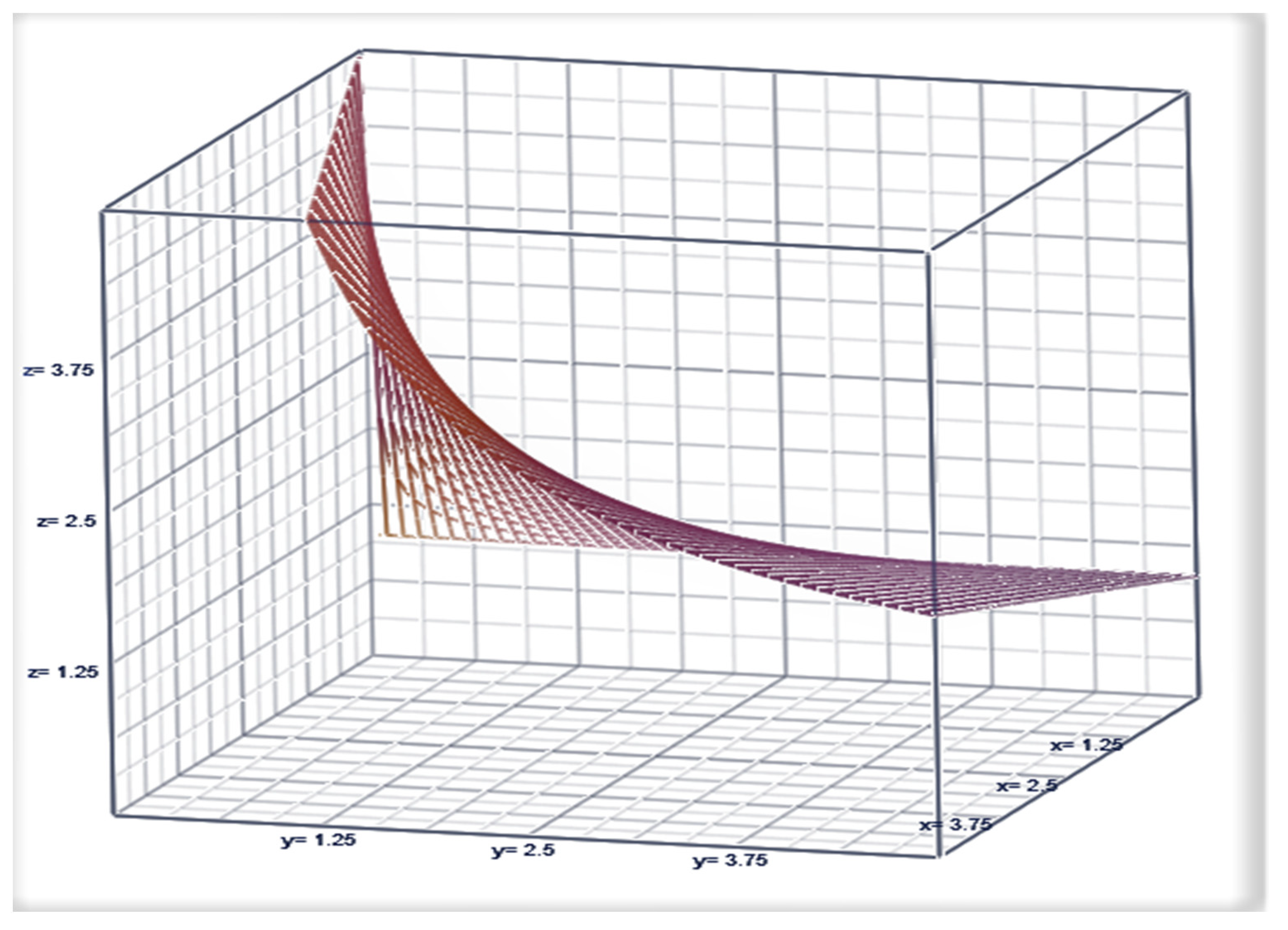
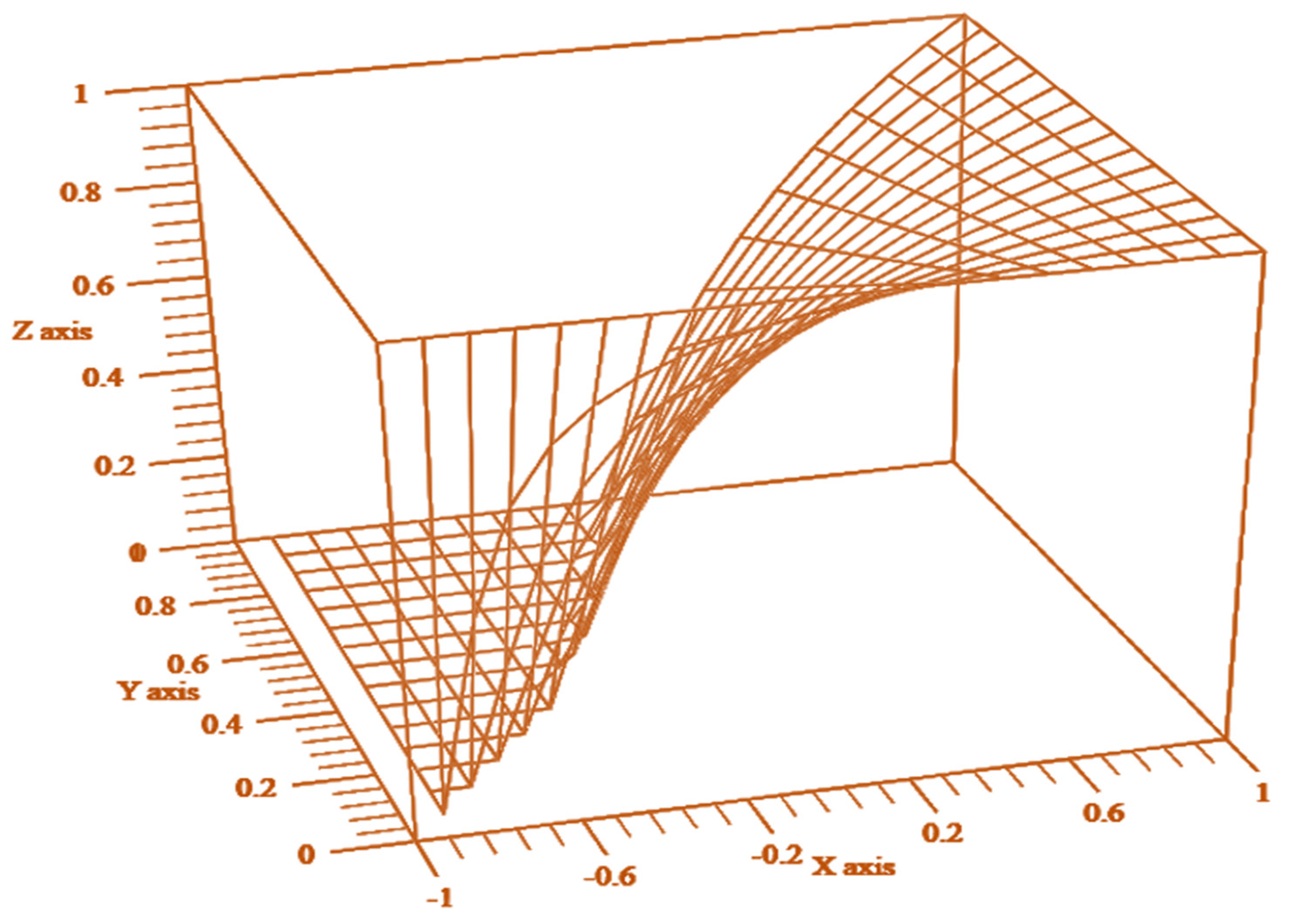
We name the factor $\Re =\left(\frac{\rho }{1+\rho }\right)\left(1+\frac{\upsilon }{\mu }\right)$ as a unique deflated risk level to die in COVID pandemic because of the efforts by the health professionals. In the deflated risk to die of COVID in a county during the pandemic, the co-proportion ${\Im }_{efforts-index}=\left(\frac{\rho }{1+\rho }\right)$ in interval [0, 1] gets the name efforts index and the other co-factor could be named pandemic index ${\Im }_{pandemic-index}=\left(1+\frac{\upsilon }{\mu }\right)$. The nonlinear configuration of the pandemic index is seen in Figure 2.

Figure 2. The nonlinear configuration of the pandemic index ${\Im }_{pandemic-index}$. The pandemic-index ${\Im }_{pandemic-index}=\left(1+\frac{\upsilon }{\mu }\right)$ is in vertical z-axis, μ and v are in the breath and x-axes respectively.

The genesis of IPD (intervened Poisson distribution) follows. With no intervention efforts, the expected number of deaths would have been just the incident rate (θ). The intervention efforts impact the expected deaths to change to ρθ. When the intervention parameter ρ is less than one, the efforts have been effective, as the expected number of deaths (after the intervention) reduced. When the intervention parameter ρ is greater than one, the variance is still less than the mean, but the scenario is indicative of inefficient efforts. Hence, we the analysis proceeds in two steps. When variance is less than one, the IPD is the underlying model for the pattern of COVID-19 deaths. When the intervention parameter is less than one, the efforts were effective. Otherwise (that is, when the intervention parameter is greater than one and the variance is lesser than the mean), the efforts were inefficient.

2.3. Estimating the Efficacy Parameter

In this section, we provided an innovative approach to estimate the IPD’s parameters using R Statistical Software [9] and the nloptr non-linear optimization package [16]. First, we cite below the major expressions to be exercised to obtain the estimates of the mortality parameter,$\theta ,$and the efficacy parameter, $\rho ,$ from the data mean, $\stackrel{-}{y,}$ and data variance, $s_y^2,$ of the COVID deaths in a county. The mean and the variance are $\mu =E\left(Y\right)=\theta [1+\rho +\left(e^{\theta }-1{)}^{-1}\right]$ and $\upsilon =Var\left(Y\right)=E\left(Y\right)-e^{\theta }{(\frac{\theta }{e^{\theta }-1})}^2$. The p-value of the data based estimate, $\widehat{\rho }$ is computed using the expression $Z_{\widehat{\rho }}=\{\frac{1}{\widehat{\rho }}{\displaystyle \sum }_{i=1}^n\frac{y_i{\widehat{\rho }}^{y_i}}{\left(1+{\widehat{\rho }}^{y_i}\right)-{\widehat{\rho }}^{y_i}}-n)\}\sqrt{\{\frac{1+\widehat{\rho }\stackrel{-}{y}}{n\widehat{\rho }\left(\stackrel{-}{y}-1\right)}\}}$, which was derived by Shanmugam [11] using the so called Neyman’s $C\left(\alpha \right)$ procedure. The p-value is the left tail probability area, $\mathit{Pr}(Z<z_{\widehat{\rho }})$ under the standard Gaussian frequency curve.

2.4. Data

Daily COVID-19 fatality data were obtained from USA Facts [17] where were compiled from the Centers for Disease Control and Prevention (CDC) [18] at the county level for all United States counties from 28 March 2020 through 26 January 2022. County-level data were selected to prevent smoothing due to aggregation, which would be associated with filtering out the ineffectiveness of the prevention efforts. This study specifically focuses on the United States, as disparate control efforts were implemented from state to state and county to county. In many more homogenous countries, controls were constant. One-hundred and thirty-seven counties with the variance less than the mean were retained to develop the inefficiency index, as this is a characteristic of the IPD. A variance greater than the mean implies efficiency in interventions. Further, when the variance is less than the mean, there is evidence that a pure Poisson process is not appropriate. In the pure Poisson process, the mean and variance should be equal, and this equality is the characteristic property. In the COVID-19 data for some counties in US, this characteristic property is not met and is thus indicative of the reality that the data deviated from the Poisson process.

3. Results

3.1. Map of Counties with Potentially Ineffective Interventions

The 137 counties retained in the study where the mean exceeds the variance are depicted in Figure 3 with shading associated with logarithm of the sum of their deaths. Many of the observations are located in the center of the country. The large majority of the counties are in the central United States. The interactive plots designed with leaflet [19] are available online [20].

Figure 3. Counties where the mean is greater than the variance.

3.2. Estimation of Parameters

To estimate both θ and ρ for each county, a positive semi-definite non-linear objective was formed that minimized the squared difference (sum of squares) between $\mu =E\left(Y\right)=\theta [1+\rho +\left(e^{\theta }-1{)}^{-1}\right]$, as specified previously, and the observed mean mortality ($\overline{X})$ for each of the counties: $Mi{n}_{\theta ,\rho }(\theta {\left[1+\rho +\left(e^{\theta }-1{)}^{-1}\right]-\overline{X}\right)}^2$. For each county, the objective function was solved using Constrained Optimization by Local Approximation (COBYLA), a derivative-free optimization algorithm developed by Powell [21] and implemented in nloptr [16]. While we might have chosen one of a number of optimization algorithms, we chose COBYLA, as it does not require gradient specification. The code is available for review online [20].

3.3. Analysis of COVID Fatalities

In the illustration, we considered COVID deaths in all counties of USA from 22 January 2020 till 9 November 2022. There were approximately 3142 counties in USA with COVID deaths in the above specified duration; however, there were another 50 observations, one per state, reflecting fatalities unallocated to a specific county. Descriptive statistics are shown in Table 1.

Table 1. Descriptive statistics.

Variable (n = 3192 Counties)	Mean	SD	Median	Sum/Rate
County Population	102,905.20	331,222.69	25,177.50	328,473,403
Sum of Fatalities	330.200	1301.39	102.00	1,054,320
Fatalities per 100,000 residents	339.32	337.10	258.71	320.98 per 100 K

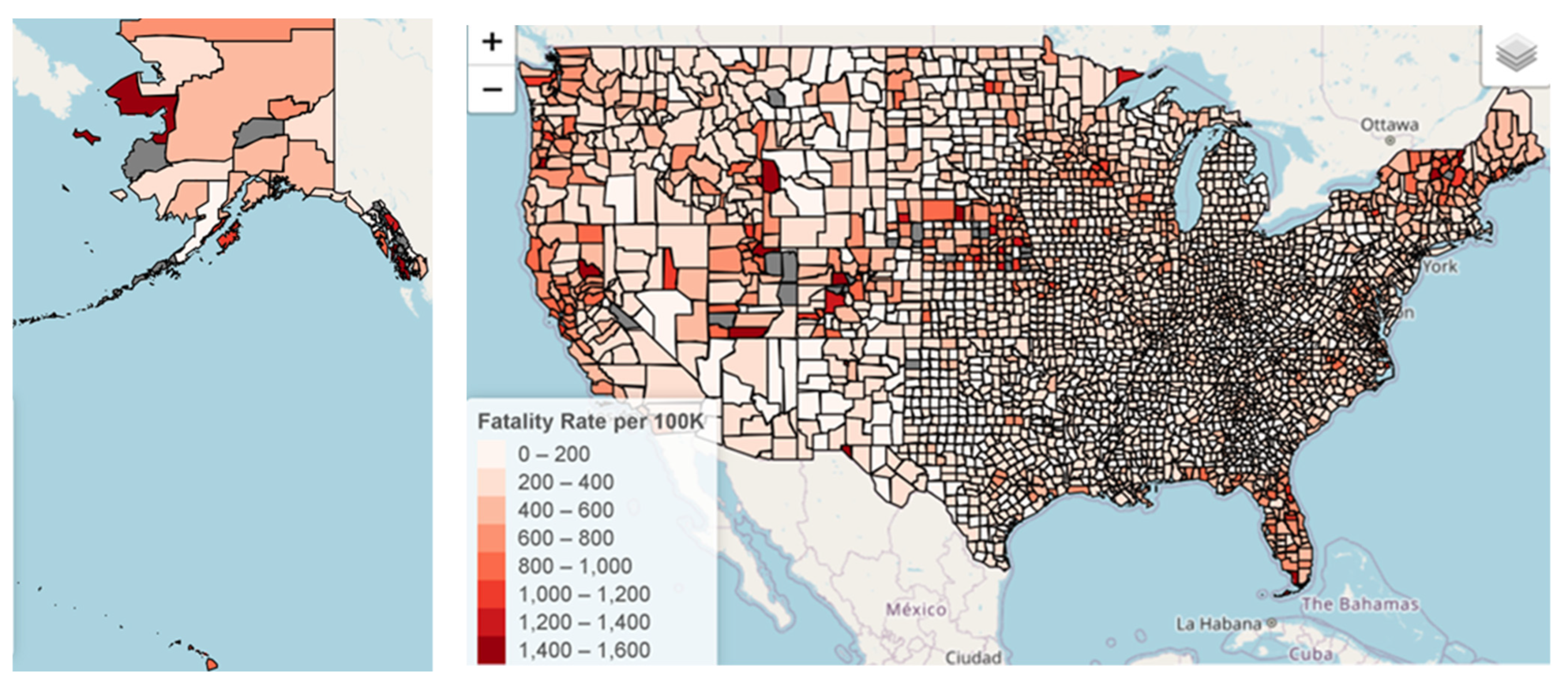
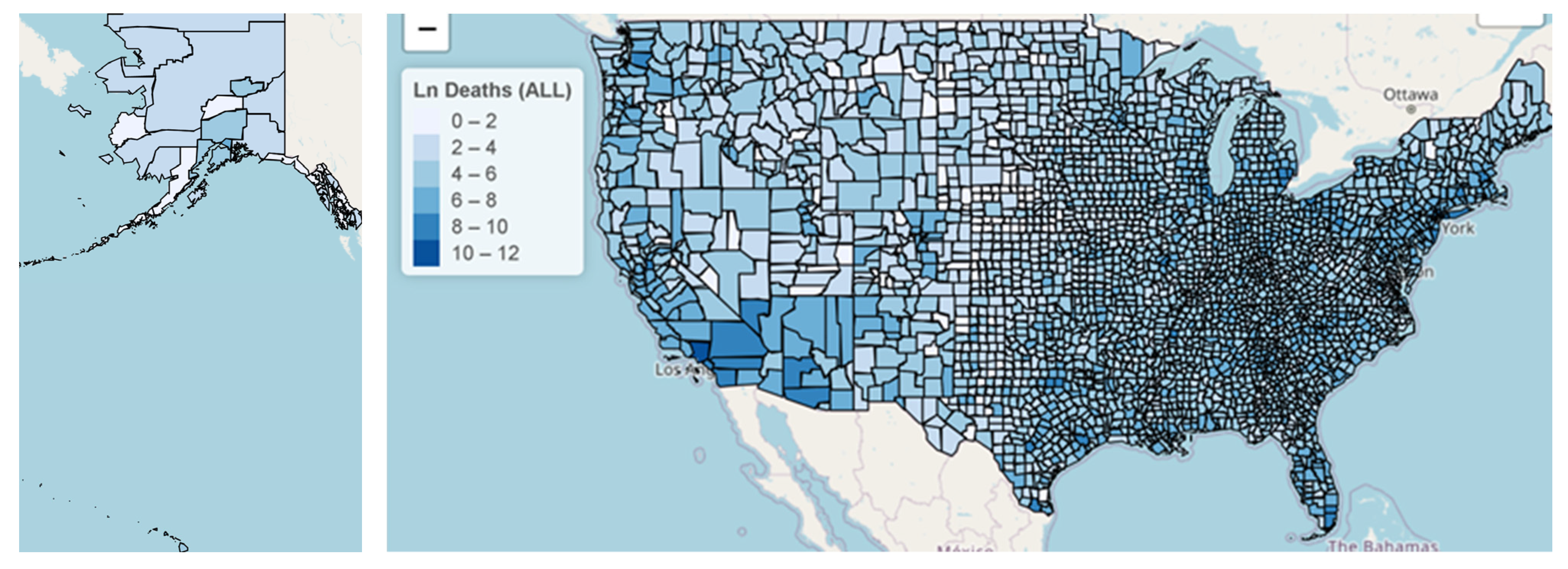
The population in this study was 328.5 million representing the United States population. The ‘average’ county was about 103 thousand (median ~25 thousand) in population and experienced 330 deaths (median of 102). The rate of fatalities per 100,000 population was about 339 on average (median of 259), and the overall fatality rate per 100,000 was 321. The fatality rates per 100,000 and logarithm of the sum of the total fatalities (+1) are depicted in Figure 4 and Figure 5.

Figure 4. COVID-19 Fatality Rate per 100,000 population (county level). NOTE: counties in gray have in excess of 1600 fatalities per 100,000.

Figure 5. COVID-19 Logarithm of the Sum of Deaths (+1).

Aggregated at the state level, fatality rates per 100,000 individuals (not adjusted for age) were highest in Mississippi (436.54), West Virginia (420.61), Alabama (419.28), and Arizona (414.97), while they were lowest in Hawaii (121.2), Vermont (122.28), Utah (157.99), and Alaska (184.68). Table 2 provides a complete enumeration of deaths, populations, and fatality rates per 100,000, while Figure 6 provides a map of the logarithm of the sum of COVID-19 Deaths (+1) for counties where the mean is greater than the variance (N = 137).

Table 2. Deaths, population, and fatality rate per 100,000 persons (sorted by fatality rate).

State	∑Deaths	Population	Rate/100 K	State	∑Deaths	Population	Rate/100 K
MS	12,992	2,976,149	436.54	MO	19,993	6,137,428	325.76
WV	7538	1,792,147	420.61	IA	10,229	3,155,070	324.21
AL	20,558	4,903,185	419.28	DE	3148	973,764	323.28
AR	12,523	3,017,804	414.97	IL	39,381	12,671,821	310.78
NM	8675	2,096,829	413.72	CT	11,034	3,565,287	309.48
TN	28,113	6,829,174	411.66	TX	89,662	28,995,881	309.22
AZ	29,852	7,278,717	410.13	MA	21,035	6,892,503	305.19
MI	39,574	9,986,857	396.26	ID	5237	1,787,065	293.05
NJ	34,940	8,882,190	393.37	ND	2232	762,062	292.89
LA	18,136	4,648,794	390.12	WI	15,516	5,822,434	266.49
KY	17,363	4,467,673	388.64	VA	22,231	8,535,519	260.45
FL	82,541	21,477,737	384.31	NC	27,264	10,488,084	259.95
GA	40,449	10,617,423	380.97	MD	15,578	6,279,560	248.07
OK	14,992	3,956,971	378.88	CA	95,990	39,512,223	242.94
NV	11,580	3,080,156	375.96	NE	4562	1,934,408	235.83
NY	73,097	19,453,561	375.75	CO	13,409	5,758,736	232.85
PA	47,994	12,801,989	374.89	MN	12,806	5,639,632	227.07
IN	24,950	6,732,219	370.61	OR	8726	4,217,737	206.89
RI	3698	1,059,361	349.08	NH	2761	1,359,711	203.06
SD	3078	884,659	347.93	ME	2711	1,344,212	201.68
SC	17,869	5,148,714	347.06	DC	1392	705,749	197.24
OH	40,249	11,689,100	344.33	WA	14,653	7,614,893	192.43
MT	3577	1,068,778	334.68	AK	1351	731,545	184.68
WY	1917	578,759	331.23	UT	5065	3,205,958	157.99
KS	9620	2,913,314	330.21	VT	763	623,989	122.28
				HI	1716	1,415,872	121.2

Figure 6. Logarithm of the Sum of COVID-19 Deaths (+1) for counties where the mean is greater than the variance (N = 137).

After finding the mean, $\stackrel{-}{y}$ and dispersion, $s_y^2$, we eliminated all those counties in which the dispersion is more than the mean. In other words, we screened and selected the counties with under dispersion, which is a requirement for the IPD model. Exactly 137 counties had under dispersion. These counties are depicted in Figure 6 and online.

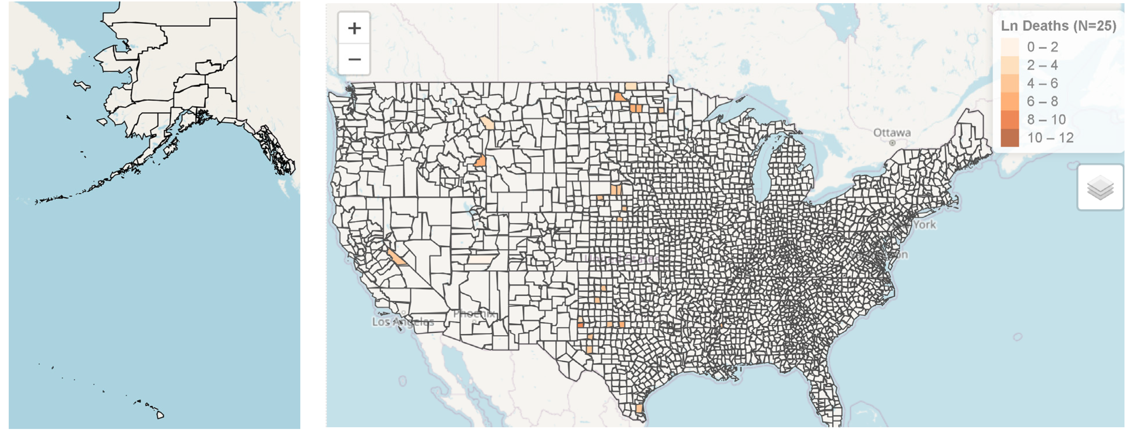
The efficacy and the mortality parameters of these counties were estimated using nonlinear optimization as described previously. Of the 137 counties which were observed to have under dispersion, only 25 were statistically significant at the α = 0.05 level. The estimates for the statistically significant counties are summarized in Table 3 and depicted in Figure 7.

Table 3. Summary of county, state, n, dispersion, mean, estimate of efficacy of efforts, p-value for COVID mortality.

County	State	${\mathit{s}}_{\mathit{y}}^2$	$\stackrel{\mathbf{-}}{\mathit{y}}$	$\widehat{\mathit{\theta }}$	$\widehat{\mathit{\rho }}$	p-Value
Mono	CA	0.00681	0.00685	0.00183	0.03846	0.023
Fremont	ID	0.02852	0.02935	0.00776	0.08412	0.032
Mahnomen	MN	0.01732	0.01761	0.00468	0.06017	0.027
Humphreys	MS	0.04588	0.04599	0.01244	0.01312	<0.001
Meagher	MT	0.00970	0.00978	0.00261	0.03624	<0.001
Brown	NE	0.00196	0.00196	0.00052	0.02345	0.037
Hooker	NE	0.00196	0.00196	0.00052	0.02345	0.037
Phelps	NE	0.00970	0.00978	0.00261	0.03624	<0.001
Rock	NE	0.00196	0.00196	0.00052	0.02345	<0.001
Sherman	NE	0.00390	0.00391	0.00104	0.04787	0.043
Camden	NC	0.00970	0.00978	0.00261	0.03624	0.001
Benson	ND	0.02202	0.02250	0.00606	0.01428	<0.001
Cavalier	ND	0.00681	0.00685	0.00183	0.03846	0.004
Griggs	ND	0.00196	0.00196	0.00052	0.02345	<0.001
Steele	ND	0.00196	0.00196	0.00052	0.02345	<0.001
Armstrong	TX	0.00970	0.00978	0.00261	0.03624	<0.001
Cochran	TX	0.02202	0.02250	0.00606	0.01428	<0.001
Kenedy	TX	0.00196	0.00196	0.00052	0.02345	<0.001
Martin	TX	0.02482	0.02544	0.00688	0.00024	<0.001
Roberts	TX	0.00196	0.00196	0.00052	0.02345	0.037
Stonewall	TX	0.00681	0.00685	0.00183	0.03846	0.023
Throckmorton	TX	0.00970	0.00978	0.00261	0.03624	0.012
Upton	TX	0.01732	0.01761	0.00468	0.06017	0.027
Yoakum	TX	0.03945	0.04110	0.01092	0.07399	<0.001
Garfield	UT	0.00970	0.00978	0.00261	0.03624	<0.001

Figure 7. Logarithm of the Sum of COVID-19 Deaths (+1) for N = 25 counties where the mean is greater than the variance and with p < 0.05.

4. Discussion

The IPD provides a probabilistic method for indexing inefficacious response efforts during pandemics. In our analysis, we discovered that 25 of the 137 counties were likely inefficient. By identifying these counties during a pandemic, efforts to identify and address the inefficiencies might be pursued. Since COVID-19 is likely not to be the last pandemic, the index generated by our analysis will be useful for future pandemics.

Some of these counties may have reasonable explanations for under dispersion. For example, Mono County, California experienced extreme particulate matter due to the wildfires in 2020, and COVID-19 deaths on these ‘wildfire days’ were higher [22]. Thus, a sustained high level of COVID-19 fatalities might be associated with environmental conditions. Kenedy, Texas was considered ‘high-risk’ for transmission of COVID-19 for various reasons, and thus might have experienced under dispersion [23]. Garfield County, Utah experienced a decline in population due to death during the pandemic [24], which might be due to pandemic prevention efforts themselves. Hooker County, Nebraska was previously identified as a high-incident outlier [25]. Neighboring Brown County may be associated with the same problematic interventions. Many of the counties in Texas had populations with high-risk comorbidities [26]. Failure to implement effective prevention measures might have exacerbated death rates. Other counties would need additional investigation to determine explanations.

5. Conclusions

COVID-19 is only a single pandemic; however, it resulted in the death of millions. The ability to identify efficacy of prevention measures using distributions, such as the IPD is critical to policymakers, as a finite number of assets are available for intervention. The human suffering and mortality rate had shaken the trust and peace of mind in everyone. Government agencies did formulate and implement preventive and treatment policies; however, the assessment of these policies might have been assisted through the use of mathematical models, such as the IPD. Policies that were assumed to be effective might have been rapidly assessed using reasonable probability distribution assumptions.

The study is based on secondary analysis, which is common when experimental designs are infeasible. Still, the classification of inefficacious versus efficacious is based on a reasonable probability model that might be affected by other factors not included in the study. Additional models would probe this limitation further. Finally, the study is limited by the validity of the data collected by the Centers for Disease Control and Prevention, although the results are likely not influenced largely by accidental input errors.

The findings in this research article identified those United States counties in which the efforts to stop the escalation of COVID-19 mortality were inefficient. In this research process, we have created an approach of indexing the inefficiency of the healthcare operations during a pandemic prior to formal modeling. This index might be used in future pandemics to identify those entities which are implementing inefficacious policies. The index can provide decision makers areas that require interventional assistance. The techniques proffered herein should prove useful for indexing efforts in future pandemics.

References

- Le, T.T.B.; Vasanthakumaran, T.; Hien, H.N.T.; Hung, I.C.; Luu, M.N.; Khan, Z.A.; An, N.T.; Tran, V.P.; Lee, W.J.; Aziz, J.M.A. SARS-CoV-2 omicron and its current known unknowns: A narrative review. Rev. Med. Virol. 2022, e2398. [Google Scholar] [CrossRef] [PubMed]
- WHO. Who Coronavirus (COVID-19) Dashboard. 2022. Available online: https://covid19.who.int/ (accessed on 2 November 2022).
- Rajan, S.; McKee, M.; Hernández-Quevedo, C.; Karanikolos, M.; Richardson, E.; Webb, E.; Cylus, J. What have european countries done to prevent the spread of COVID-19? Lessons from the COVID-19 health system response monitor. Health Policy 2022, 126, 355–361. [Google Scholar] [CrossRef] [PubMed]
- Unruh, L.; Allin, S.; Marchildon, G.; Burke, S.; Barry, S.; Siersbaek, R.; Thomas, S.; Rajan, S.; Koval, A.; Alexander, M. A comparison of 2020 health policy responses to the COVID-19 pandemic in canada, ireland, the united kingdom and the united states of america. Health Policy 2022, 126, 427–437. Available online: https://www.ncbi.nlm.nih.gov/pmc/articles/PMC9187506/pdf/main.pdf (accessed on 2 November 2022). [CrossRef] [PubMed]
- Jiao, J.; Shi, L.; Zhang, Y.; Chen, H.; Wang, X.; Yang, M.; Yang, J.; Liu, M.; Sun, G. Core policies disparity response to COVID-19 among brics countries. Int. J. Equity Health 2022, 21, 9. [Google Scholar] [CrossRef] [PubMed]
- Brauner, J.M.; Mindermann, S.; Sharma, M.; Johnston, D.; Salvatier, J.; Gavenčiak, T.; Stephenson, A.B.; Leech, G.; Altman, G.; Mikulik, V. Inferring the effectiveness of government interventions against COVID-19. Science 2021, 371, eabd9338. Available online: https://www.ncbi.nlm.nih.gov/pmc/articles/PMC7877495/pdf/371_abd9338.pdf (accessed on 2 November 2022). [CrossRef] [PubMed]
- Feinhandler, I.; Cilento, B.; Beauvais, B.; Harrop, J.; Fulton, L. Predictors of death rate during the COVID-19 pandemic. Presented Healthc. 2020, 8, 339. [Google Scholar] [CrossRef] [PubMed]
- McAleer, M. Prevention is better than the cure: Risk management of COVID-19. J. Risk Financ. Manag. 2020, 13, 46. [Google Scholar] [CrossRef]
- R Development Core Team. R: A Language and Environment for Statistical Computing; R Development Core Team: Vienna, Austria, 2018. [Google Scholar]
- Shanmugam, R. An intervened poisson distribution and its medical application. Biometrics 1985, 41, 1025–1029. Available online: http://www.jstor.org/stable/2530973 (accessed on 2 November 2022). [CrossRef] [PubMed]
- Shanmugam, R. An inferential procedure for the poisson intervention parameter. Biometrics 1992, 48, 559–565. [Google Scholar] [CrossRef] [PubMed]
- Joyce, V.J.; Merlin, G.S.; Edna, K.R.J.; Fenella, S. Designing mixed sampling plan based on ipd. J. Manag. Inf. Decis. Sci. 2021, 24, 1–6. [Google Scholar]
- Shanmugam, R. Revelation of shrunken or stretched binomial dispersion and public perception of situations which might spread aids or hiv. Int. J. Res. Med. Sci. 2014, 2, 462–467. [Google Scholar] [CrossRef][Green Version]
- Shanmugam, R. Modelling web changes data recatched during a spread of internet virus. Math. Comput. Model. 2005, 42, 1175–1190. [Google Scholar] [CrossRef]
- Shanmugam, R. Predicting “successful” prevention of an epidemic. Commun. Stat.-Theory Methods 2006, 30, 93–103. [Google Scholar] [CrossRef]
- Johnson, S.G. The Nlopt Nonlinear Optimization Package. 2022. Available online: https://nlopt.readthedocs.io/en/latest/ (accessed on 2 November 2022).
- Usafacts. Us COVID-19 Cases and Deaths by State. 2022. Available online: https://usafacts.org/visualizations/coronavirus-COVID-19-spread-map (accessed on 2 November 2022).
- CDC. Trends in Number of COVID-19 Cases and Deaths in the Us Reported to CDC, by State/Territory. 2022. Available online: https://covid.cdc.gov/covid-data-tracker/#trends_weeklydeaths_select_00 (accessed on 2 November 2022).
- Cheng, J.; Karambelkar, B.; Xie, Y. Leaflet: Create Interactive Web Maps with the Javascript ‘Leaflet’ Library, 2022.
- Fulton, L. Rpubs Code. 2022. Available online: https://rpubs.com/R-Minator/Ram22 (accessed on 2 November 2022).
- Powell, M.J. A view of algorithms for optimization without derivatives. Math. Today-Bull. Inst. Math. Appl. 2007, 43, 170–174. [Google Scholar]
- Zhou, X.; Josey, K.; Kamareddine, L.; Caine, M.C.; Liu, T.; Mickley, L.J.; Cooper, M.; Dominici, F. Excess of COVID-19 cases and deaths due to fine particulate matter exposure during the 2020 wildfires in the united states. Sci. Adv. 2021, 7, eabi8789. [Google Scholar] [CrossRef] [PubMed]
- Rao, S.; Singh, M.; Hemnani, K.; Arroyo, C. Can we abandon our masks? Deciphering cdc’s new guidelines about masking. DHR Proc. 2022, 2, 1–3. [Google Scholar] [CrossRef]
- Lake, S.; Juan, A.S. State and county population estimates for utah: 2021. Population 2021, 3, 3–4. [Google Scholar]
- Andrews, M.R.; Tamura, K.; Best, J.N.; Ceasar, J.N.; Batey, K.G.; Kearse, T.A., Jr.; Allen, L.V., III; Baumer, Y.; Collins, B.S.; Mitchell, V.M. Spatial clustering of county-level COVID-19 rates in the us. Int. J. Environ. Res. Public Health 2021, 18, 12170. Available online: https://mdpi-res.com/d_attachment/ijerph/ijerph-18-12170/article_deploy/ijerph-18-12170-v3.pdf?version=1637639494 (accessed on 2 November 2022). [CrossRef] [PubMed]
- Chin, T.; Kahn, R.; Li, R.; Chen, J.T.; Krieger, N.; Buckee, C.O.; Balsari, S.; Kiang, M.V. US county-level characteristics to inform equitable COVID-19 response. medRxiv 2020. [Google Scholar] [CrossRef]
Publisher’s Note: MDPI stays neutral with regard to jurisdictional claims in published maps and institutional affiliations. |
© 2022 by the authors. Licensee MDPI, Basel, Switzerland. This article is an open access article distributed under the terms and conditions of the Creative Commons Attribution (CC BY) license (https://creativecommons.org/licenses/by/4.0/).