Optimal Per-Loss Reinsurance for a Risk Model with a Thinning-Dependence Structure

Abstract

In this paper, we consider the optimal reinsurance problem for a risk model with a thinning-dependence structure, where the stochastic sources related to claim occurrence are classified into different groups, and each group may cause a claim in each insurance class with some probability. We assume that the insurer can manage the risk by purchasing per-loss reinsurance, and their aim is to maximize the expected utility of the terminal wealth. By using the technique of stochastic control, we obtain the corresponding Hamilton–Jaccobi–Bellman equation. From the perspective of game theory, we derive the closed-form expression of the optimal strategy for each class of business, which is actually the best response to other given strategies. We also investigate the necessary conditions for optimal strategies and transfer the original optimization problem into a system of equations. Furthermore, we prove that the solution of the system of equations always exists, but may not be unique, and we also study some features of the optimal strategies in special cases and derive several interesting results. Finally, some numerical examples are given to show the impacts of some important parameters on the optimal strategies.

1. Introduction

Over recent decades, optimal reinsurance problems have received much attention in actuarial study. Insurers can control risks by purchasing reinsurance, and popular criteria minimize the probability of ruin, thus maximizing the expected utility and mean-variance criterion; see, for example [1,2,3,4,5,6,7], etc. Recently, some researchers studied dependent classes of businesses that can describe risk claims more precisely for insurers. One dependent risk model is the so-called common shock, namely, there are different business risks as a result of one stochastic source. For this risk model, ref. [8] found the optimal dynamic excess-of-loss reinsurance under the criterion of minimizing the ruin probability for a diffusion model; ref. [9] investigated the optimal proportional reinsurance that maximizes the expected utility of terminal wealth for both compound Poisson and diffusion approximation risk models with the variance premium principle; ref. [10] studied optimal mean-variance reinsurance and investment in a jump-diffusion financial market; ref. [11] obtained the optimal proportional reinsurance for minimizing the probability of drawdown.

In order to describe the more realistic features of dependence, ref. [12] proposed a risk model with thinning dependence, that is, one event may induce some different classes of business risks with certain probabilities. One of the typical examples is that a severe traffic accident may cause not only the loss of a damaged car, but also the medical expenses of injured drivers and passengers. For the thinning model, refs. [13,14] considered the optimal proportional reinsurance under the criteria of maximizing the adjustment coefficient and minimizing the probability of drawdown, respectively; ref. [15] studied the optimal reinsurance strategies for the mean-variance criterion.

Much of the existing literature, like the studies mentioned above, studied optimal problems with some specific form of reinsurance, such as proportional reinsurance, excess-of-loss reinsurance, or a combination of the two. Recently, some scholars studied optimal reinsurance strategies with various objectives but without a constraint on the reinsurance form, which is called the per-loss reinsurance. The main method of obtaining optimal per-loss reinsurance strategies is the pointwise optimization method, which can also be understood as the specific Euler–Lagrange equation in classical calculus of variations. For example, ref. [16] investigated the optimal investment and reinsurance strategies for insurers with a generalized mean-variance premium principle and no-short selling; ref. [17] studied the optimal per-loss reinsurance with the criterion of minimizing the probability of ruin; ref. [18] considered the optimal reinsurance strategy in order to minimize the drawdown probability with the mean-variance premium principle. However, very few of them considered the optimal per-loss reinsurance for dependent risk models, which are more beneficial for real insurance markets. Meanwhile, in mathematics, deriving several optimal controls that affect each other is more difficult and challenging than deriving independent controls.

In this paper, we consider the optimal per-loss reinsurance in order to maximize the expected utility of terminal wealth with a thinning-dependence structure, and the reinsurance premium is computed according to the mean-variance premium principle. By using stochastic control theory, we establish the corresponding Hamilton–Jacobi–Bellman equation for both the compound Poisson thinning model and its diffusion approximation. Via the pointwise optimization method, we obtain the closed-form expression of the optimal strategy for each business that is expressed by other given strategies, or, we can say, it is the best response to other strategies, such as in game theory. Then, we derive the necessary conditions for the optimal strategies. For the compound Poisson model, we obtain an system of equations with respect to the moment-generating functions of the optimal strategies; for the diffusion approximation model, we get a system of equations about the expectations of the optimal strategies. We prove that the solution of this equation system always exists, but may not be unique. However, for some special cases, this uniqueness is established, such as with the diffusion approximation risk model with only two classes of insurance businesses, or when there is only one group of stochastic sources and the variance safety loadings for all insurance classes are the same. For the latter case, we also find that when the number of business classes is increased, all of the original optimal retained strategies are decreased in order to balance the risk.

In addition, for the diffusion approximation risk model, we can see that the optimal strategy is actually a combination of the excess-of-loss reinsurance and the proportional reinsurance. When the mean-variance premium principle is reduced to the expected value principle, the optimal strategy becomes the excess-of-loss reinsurance. However, when it becomes the variance premium principle, the optimal strategy is not a proportional reinsurance anymore; instead, the insurer will choose to transfer all of the small-size claims and retain a portion of the excess. Moreover, we compare the optimal strategies of the dependent risk model and independent risk model with those of the jump model and the diffusion model, respectively. The results show that the optimal retained strategy for the former case is always smaller than the one for the latter.

The remainder of the paper is organized as follows. In Section 2, we introduce the thinning model and the problem formulation. In Section 3 and Section 4, we derive the closed-form expressions of the optimal strategies for both the compound Poisson and diffusion approximation risk models, and we obtain the necessary conditions that the optimal strategies must satisfy. In Section 5, we provide some numerical examples to show the properties of the optimal strategies and analyze the influences of some important parameters on the optimal strategies. Finally, we conclude this paper and raise some questions for further discussion in Section 6.

2. Model Setup and Problem Formulation

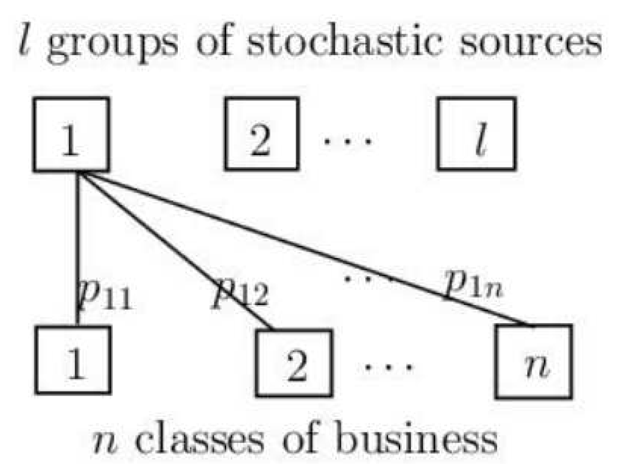
In this section, we will introduce the thinning-dependence model that was firstly proposed by [12]. Suppose that an insurance company has n dependent classes of businesses, such as health insurance businesses, life insurance businesses, etc., and there are l groups of stochastic sources that may affect some of these insurance businesses with a certain probability (see Figure 1). In this setting, we use $N^k\left(t\right)$ to denote the number of events from the kth group that occur up to time t, where $k\in \{1,2,\dots ,l\}$. Let $N_j^k\left(t\right)$ be the number of claims for the jth class up to time t generated by the kth stochastic source. Then, the claim-number process $N_j\left(t\right)$ for the jth business class of the insurance company can be described by

$$N_j\left(t\right)=N_j^1\left(t\right)+N_j^2\left(t\right)+\cdots +N_j^l\left(t\right).$$

Moreover, it is assumed that $N^1\left(t\right),N^2\left(t\right),\dots ,N^l\left(t\right)$ are independent Poisson processes with intensities ${\lambda }_1,{\lambda }_2,\dots ,{\lambda }_l$, and thus, $N_j^k\left(t\right)$ is a time-homogeneous Poisson process with intensity ${\lambda }_k{p}_{kj}$. Here, $p_{kj}$ represents the probability of the event that the kth risk source affects the jth business’s claim, and $N_j^k\left(t\right)$ is the $p_{kj}$-thinning of $N^k\left(t\right)$. It is reasonable to further assume that the components of the vector of a claim-number process, $(N_1^k\left(t\right),N_2^k\left(t\right),\dots ,N_n^k\left(t\right))$, are conditionally independent given $N^k\left(t\right)$.

Here, we further explain the two independence assumptions mentioned above. The independence among $N^1\left(t\right),\dots ,N^l\left(t\right)$ means that different groups of stochastic sources do not affect each other. For example, we suppose that $N^1\left(t\right)$ represents the number of traffic accidents and $N^2\left(t\right)$ represents the number of epidemics; then, it is rational to assume that they are independent of each other. The independence of $(N_1^k\left(t\right),N_2^k\left(t\right),\dots ,N_n^k\left(t\right))$ when given $N^k\left(t\right)$ means that the events of the kth group will independently trigger different classes of insurance. For instance, we suppose that $N^k\left(t\right)$ represents the number of traffic accidents, $N_1^k\left(t\right)$ denotes the claim number generated by traffic accidents for auto insurance, and $N_1^k\left(t\right)$ denotes the claim number generated by traffic accidents for life insurance. Then, it is reasonable to think that whether a traffic accident will trigger the auto insurance is independent of whether it will trigger the life insurance.

Let $Y_j\left(i\right)$ be the claim size, which is a random variable for the ith claim in the jth class. Then, the total number of claims from the jth class up to time t can be expressed as

$$S_j\left(t\right)=\sum _{i=1}^{N_j\left(t\right)}{Y}_j\left(i\right).$$

Therefore, the aggregate claims process of the company is given by

$$S\left(t\right)=\sum _{j=1}^n\sum _{i=1}^{N_j\left(t\right)}{Y}_j\left(i\right),$$

where $\{Y_j\left(i\right)\ge 0;i=1,2,\dots ,n\}$ are a sequence of i.i.d positive random variables with a common distribution $F_j$. Let ${\mu }_j,{\sigma }_j^2$, and $M_{Y_j}\left(r\right)$ denote its the first- and second-order moments and the moment-generating function, respectively. As usual, we assume that the n sequences are mutually independent and are independent of all claim-number processes.

Now, we define the surplus process of the insurance company as

$$R\left(t\right)=u+ct-S\left(t\right),$$

(1)

where u is the initial wealth, and c is the premium rate. In this paper, we suppose that the insurance company can manage its risk by purchasing per-loss reinsurance via a continuously payable premium, which is computed according to the mean-variance premium principle. The insurer retains $\left(I_1\left(Y_1\right),\dots ,I_n\left(Y_n\right)\right)$ for the n business claims, where $I_j$ is a function of $Y_j$ for $j\in \{1,2,\dots ,n\}$, and the remaining losses $\left(Y_1-I_1\left(Y_1\right),\dots ,Y_n-I_n\left(Y_n\right)\right)$ are ceded to the reinsurer. Furthermore, the insurer is allowed to invest all of its wealth into a risk-free asset with an interest rate r. Let $R^I\left(t\right)$ denote the associated surplus process under the reinsurance strategy $I_1\left(Y_1\right),\dots ,I_n\left(Y_n\right)$; then, it evolves as

$$d{R}^I\left(t\right)=[r{R}^I\left(t\right)+c-\sum _{j=1}^{n}p\left(I_j\left(Y_j\right)\right)]dt-d\sum _{j=1}^n\sum _{i=1}^{N_j\left(t\right)}{I}_j\left(Y_j\right),$$

(2)

where

$${\displaystyle p\left(I_j\left(Y_j\right)\right)=\sum _{k=1}^l{\lambda }_k{p}_{kj}\left[(1+{\theta }_j)E(Y_j-I_j\left(Y_j\right))+{\alpha }_{j}E{(Y_j-I_j\left(Y_j\right))}^2\right]}$$

is the mean-variance reinsurance premium, and ${\theta }_j,{\alpha }_j$ are safety loadings for the jth business class.

Remark 1.

If we denote ${\displaystyle S^I\left(t\right)=\sum _{j=1}^n\sum _{i=1}^{N_j\left(t\right)}{I}_j\left(Y_j\left(i\right)\right)}$, then it follows from [12] that $S^I\left(t\right)$ is also a compound Poisson process. Furthermore, it is equal in law to ${\tilde{S}}^I\left(t\right)$ given by

$${\tilde{S}}^I\left(t\right)=\sum _{i=1}^{N^Z\left(t\right)}{Z}_i,$$

where $N^Z\left(t\right)$ is a Poisson process with intensity

$${\displaystyle \lambda ={\lambda }_1+{\lambda }_2+\cdots +{\lambda }_l,}$$

$\{Z_i;i=1,2,\dots \}$ are independent with a common distribution $F_Z$, and the moment-generating function is

$$M_Z\left(r\right)=\frac{1}{\lambda }\sum _{k=1}^l{\lambda }_k\prod _{j=1}^n\left(M_{I_j\left(Y_j\right)}\left(r\right)p_{kj}+1-p_{kj}\right),$$

where ${\displaystyle M_{I_j\left(Y_j\right)}\left(r\right)={\int }_0^{\infty }{e}^{I_j\left(y\right)r}d{F}_{Y_j}\left(y\right)}$.

Let $I={(I_{1t},I_{2t},\dots ,I_{nt})}_{t\in [0,T]}$ represent the reinsurance control process selected by the insurer; then, we define the admissible strategy as follows.

Definition 1.

(Admissible control) The control $I_t=\{I_{1t},I_{2t},\dots ,I_{nt}\}$ is said to be admissible if and only if

 (1) 

for $\forall j\in \{1,2,\dots ,n\}$, $I_{jt}\left(Y_j\right)$ is increasing with respect to $Y_j$ and $0\le I_{jt}\left(Y_j\right)\le Y_j$,

 (2) 

$I_t=\{I_{1t},I_{2t},\dots ,I_{nt}\}$ is an ${\mathcal{F}}_t$-predictable process,

 (3) 

in association with $I_t$, the state Equation (2) has a unique strong solution.

The set of all admissible strategies is denoted by $\mathcal{O}$.

Suppose that the insurer is interested in maximizing the expected utility of its terminal wealth, say, at time T. We assume that the insurer has a CARA preference, i.e., they choose the exponential utility function

$$U\left(x\right)=-\frac{\rho }{\nu }{e}^{-\nu x},$$

where $\nu >0$ is constant risk aversion. For the strategy $I=(I_1,I_2,\dots ,I_n)$, we define the objective function at time t as

$$J(t,x,I)=\mathbb{E}\left[U\left(R^I\left(T\right)\right)\right|R^I\left(t\right)=x],$$

and our aim is to find the value function

$$V(t,x)=\underset{I\in \mathcal{O}}{sup}J(t,x,I)$$

and the optimal strategy $I^{\ast }=(I_1^{\ast },I_2^{\ast },\dots ,I_n^{\ast })$ such that $J(t,x,I^{\ast })=V(t,x)$.

3. Optimal Results for the Compound Poisson Model

In this section, we will discuss the optimal reinsurance problem for the compound Poisson risk model with a thinning-dependence structure. As a special case, we will also analyze the results for the classical Cramer–Lundberg (C-L) model. From the standard arguments of the dynamic programming approach (see, e.g., [19]), we see that if the optimal value function $V(t,x)$ and its partial derivatives $V_t(t,x)$ and $V_x(t,x)$ are continuous on $[0,T]\times R$, then V satisfies the following HJB equation:

$$\underset{I\in \mathcal{O}}{sup}\left\{V_t+(rx+c-\sum _{k=1}^l{\lambda }_k{p}_{kj}[(1+{\theta }_j)E(Y_j-I_j\left(Y_j\right))+{\alpha }_{j}E{(Y_j-I_j\left(Y_j\right))}^2])V_x+\lambda E[V(t,x-Z)-V(t,x)]\right\}=0,$$

(3)

with the boundary condition

$$V(T,x)=-\frac{\rho }{\nu }{e}^{-\nu x}.$$

(4)

Before solving this HJB equation, we first give a lemma that reveals some features of the optimal strategy and the conjecture of the value function $V(T,x)$.

Lemma 1.

If the insurer chooses the exponential utility function $U\left(x\right)=-\frac{\rho }{\nu }{e}^{-\nu x}$, then the optimal strategy is independent of x. Furthermore, the value function has the form of

$$V(t,x)=-\frac{\rho }{\nu }exp\left[-\nu xexp\left(r\right(T-t\left)\right)+h(T-t)\right],$$

(5)

with $h\left(0\right)=0$.

Proof. 

According to Equation (2), we know that

$$\begin{array}{cc}{R}^I\left(T\right)=\hfill & {\displaystyle x{e}^{r(T-t)}+{\int }_t^T\left(e^{r(s-t)}\left[c-\sum _{j=1}^n\sum _{k=1}^l{\lambda }_k{p}_{kj}[(1+{\theta }_j)E(Y^j-I_j\left(Y^j\right))+{\alpha }_{j}E{(Y^j-I_j\left(Y^j\right))}^2]\right]\right)ds}\hfill \\ \hfill & {\displaystyle -{\int }_t^T{\int }_0^{\infty }{e}^{r(s-t)}z{N}^Z(ds,dz),}\hfill \end{array}$$

(6)

where $N^Z(·,·)$ is the random Poisson measure such that ${\displaystyle \sum _{i=1}^{N^Z\left(t\right)}{Z}_i={\int }_0^t{\int }_0^{\infty }z{N}^Z(ds,dz)}$. Then, the value function $V(t,x)$ can be denoted by

$$\begin{array}{cc}V(t,x)\hfill & {\displaystyle =\underset{I\in \mathcal{O}}{sup}\mathbb{E}[U\left(R^I\left(T\right)\right)|R^I\left(t\right)=x]}\hfill \\ \hfill & {\displaystyle =exp\{-\nu x{e}^{r(T-t)}\}\underset{I\in \mathcal{O}}{sup}\mathbb{E}[-\frac{\rho }{\nu }exp\{-\nu {\int }_t^T\left(e^{r(s-t)}\right[c-\sum _{j=1}^n\sum _{k=1}^l{\lambda }_k{p}_{kj}[(1+{\theta }_j)E(Y^j-I_j\left(Y^j\right))}\hfill \\ \hfill & {\displaystyle +{\alpha }_{j}E{(Y^j-I_j\left(Y^j\right))}^2]])ds-\nu {\int }_t^T{\int }_0^{\infty }{e}^{r(s-t)}z{N}^Z(ds,dz)\left\}\right]}\hfill \\ \hfill & {\displaystyle :=exp\{-\nu x{e}^{r(T-t)}\}\underset{I\in \mathcal{O}}{sup}-\frac{\rho }{\nu }exp\left\{H(T-t,I)\right\},}\hfill \end{array}$$

(7)

Thus, from the last expression, we find that the optimal strategies only depend on the time t. Consequently, we can derive that the value function has the form of

$$V(t,x)=-\frac{\rho }{\nu }exp\left[-\nu xexp\left(r\right(T-t\left)\right)+h(T-t)\right],$$

(8)

where $h\left(0\right)=0$, which completes the proof. □

Next, we try to construct a solution of the HJB Equation (3) with the boundary condition (4). Suppose that $W(t,x)$ has the form of (8) and satisfies (3) and (4). Then, we have

$$\left\{\begin{array}{c}{W}_t=W(t,x)[\nu xrexp\left(r\right(T-t\left)\right)-h^{\prime }(T-t)],\hfill \\ W_x=W(t,x)[-\nu exp\left(r\right(T-t\left)\right)],\hfill \\ \mathbb{E}W(t,x-Z)=W(t,x)M_Z(\nu exp\left(r(T-t)\right)).\hfill \end{array}\right.$$

(9)

Putting them into back the HJB equation, we obtain

$$\begin{array}{c}{\displaystyle \underset{I\in \mathcal{O}(t,x)}{inf}\{-\nu e^{r(T-t)}(c-\sum _{j=1}^n\sum _{k=1}^l{\lambda }_k{p}_{kj}[(1+{\theta }_j)E(Y_j-I_j\left(Y_j\right))}\hfill \\ +{\alpha }_{j}E{(Y_j-I_j\left(Y_j\right))}^2\left]\right)+\lambda [M_Z\left(\nu e^{r(T-t)}\right)-1]\}-h^{\prime }(T-t)=0.\hfill \end{array}$$

(10)

Now, we come to find the extreme point $(I_1^{\ast },I_2^{\ast },\dots ,I_n^{\ast })$, which causes the left-hand side of (10) to be minimized. Firstly, we would like to find the best response $I_j(I_1,\dots ,I_{j-1},I_{j+1},\dots ,I_n)$ to other strategies when $I_1,\dots ,I_{j-1},I_{j+1},\dots ,I_n$ are given, as shown in the following theorem.

Theorem 1.

Given the other strategies $I_1,\dots ,I_{j-1},I_{j+1},\dots ,I_n$, we denote $a_i=M_{I_i}\left(\nu e^{r(T-t)}\right)$. Then, the best response $I_j(·,y)$ is given by

$$I_j(a_1,\dots ,a_{j-1},a_{j+1},\dots ,a_n;y)=max\left\{0,min\{y,{\tilde{I}}_j(a_1,\dots ,a_{j-1},a_{j+1},\dots ,a_n;y)\}\right\},$$

where ${\tilde{I}}_j(a_1,\dots ,a_{j-1},a_{j+1},\dots ,a_n;y)$ satisfies

$$\sum _{k=1}^l{\lambda }_k{p}_{kj}\left[2{\alpha }_j({\tilde{I}}_j-y)-(1+{\theta }_j)+exp\left(\nu e^{r(T-t)}{\tilde{I}}_j\right)\prod _{i\ne j}(1-p_{ki}+p_{ki}{a}_i)\right]=0.$$

Proof. 

Let

$$\begin{array}{cc}\varphi (t,x,I)=\hfill & {\displaystyle -\nu e^{r(T-t)}(c-\sum _{j=1}^n\sum _{k=1}^l{\lambda }_k{p}_{kj}[(1+{\theta }_j)E(Y_j-I_j\left(Y_j\right))+{\alpha }_{j}E{(Y_j-I_j\left(Y_j\right))}^2])}\hfill \\ \hfill & +\lambda [M_Z\left(\nu e^{r(T-t)}\right)-1].\hfill \end{array}$$

From (10), we can see that to find the optimal $I_j$ is to minimize

$$\begin{array}{c}\sum _{k=1}^l{\lambda }_k{p}_{kj}\nu e^{r(T-t)}E\left[(1+{\theta }_j)(Y_j-I_j)+{\alpha }_j{(Y_j-I_j)}^2\right]\hfill \\ +\sum _{k=1}^l{\lambda }_k\prod _{i=1}^n\left[M_{I_i}\left(\nu e^{r(T-t)}\right)p_{ki}+1-p_{ki}\right]\hfill \\ =E\{\sum _{k=1}^l{\lambda }_k{p}_{kj}\nu e^{r(T-t)}\left[(1+{\theta }_j)(Y_j-I_j)+{\alpha }_j{(Y_j-I_j)}^2\right]\hfill \\ +\sum _{k=1}^l{\lambda }_k\left(e^{I_j\nu e^{r(T-t)}}{p}_{kj}+1-p_{kj}\right)\prod _{i\ne j}\left[M_{I_i}\left(\nu e^{r(T-t)}\right)p_{ki}+1-p_{ki}\right]\}.\hfill \end{array}$$

According tothe pointwise optimization method, this is equivalent to minimizing the following function:

$$\begin{array}{cc}\hfill & f\left(I_j\right)=\sum _{k=1}^l{\lambda }_k{p}_{kj}\nu e^{r(T-t)}\left[(1+{\theta }_j)(Y_j-I_j)+{\alpha }_j{(Y_j-I_j)}^2\right]\hfill \\ \hfill & +\sum _{k=1}^l{\lambda }_k\left(e^{I_j\nu e^{r(T-t)}}{p}_{kj}+1-p_{kj}\right)\prod _{i\ne j}\left[M_{I_i}\left(\nu e^{r(T-t)}\right)p_{ki}+1-p_{ki}\right].\hfill \end{array}$$

Through some calculations, we find that

$$f^{\prime }\left(I_j\right)=\sum _{k=1}^l{\lambda }_k{p}_{kj}\nu e^{r(T-t)}\left[2{\alpha }_j(I_j-y)-(1+{\theta }_j)+exp\left(\nu e^{r(T-t)}{I}_j\right)\prod _{i\ne j}(1-p_{ki}+p_{ki}{M}_{I_i}\left(\nu e^{r(T-t)}\right))\right],$$

$$f″\left(I_j\right)=\sum _{k=1}^l{\lambda }_k{p}_{kj}\nu e^{r(T-t)}\left[2{\alpha }_j+\nu e^{r(T-t)}exp\left(\nu e^{r(T-t)}{I}_j\right)\prod _{i\ne j}(1-p_{ki}+p_{ki}{M}_{I_i}\left(\nu e^{r(T-t)}\right))\right]>0.$$

Therefore, for any $j\in \{1,2,\dots ,n\}$, the minimizer $I_j$ satisfies the equation

$$f^{\prime }\left(I_j\right)=0.$$

(11)

We might as well denote ${\tilde{I}}_j$ as the solution of (11), and it is affected by the other given strategies due to the term $M_{I_i}\left(\nu e^{r(T-t)}\right)$. If we denote $M_{I_i}\left(\nu e^{r(T-t)}\right)$ by $a_i$, then ${\tilde{I}}_j$ is actually a function of $a_1,\dots ,a_{j-1},a_{j+1},\dots ,a_n$ and can be written as ${\tilde{I}}_j(a_1,\dots ,a_{j-1},a_{j+1},\dots ,a_n;y)$. Considering the constraint $0\le I_j\left(y\right)\le y$, the best strategy of response $I_j(I_1,\dots ,I_{j-1},I_{j+1},\dots ,I_n)$ to other strategies is given by

$$I_j(a_1,\dots ,a_{j-1},a_{j+1},\dots ,a_n;y)=max\left\{0,min\{y,{\tilde{I}}_j(a_1,\dots ,a_{j-1},a_{j+1},\dots ,a_n;y)\}\right\},$$

(12)

which completes the proof. □

Before providing a further discussion on the extreme point, we first show some properties in Lemma 2, as they play key roles in this paper.

Lemma 2.

${\tilde{I}}_j$ is decreasing with respect to $a_m(m\ne j)$ and increasing with respect to y.

Proof. 

Recall that ${\tilde{I}}_j$ satisfies (11). Differentiating both sides of (11) with respect to $a_m$ and y, respectively, we get

$$\sum _{k=1}^l{\lambda }_k{p}_{kj}\left[2{\alpha }_j\frac{\partial {\tilde{I}}_j}{\partial a_m}+exp\left(\nu e^{r(T-t)}{I}_j\right)\nu e^{r(T-t)}\frac{\partial {\tilde{I}}_j}{\partial a_m}\prod _{i\ne j}(1-p_{ki}+p_{ki}{a}_i)+exp\left(\nu e^{r(T-t)}{I}_j\right)p_{km}\prod _{i\ne j,m}(1-p_{ki}+p_{ki}{a}_i)\right]=0,$$

and

$$\sum _{k=1}^l{\lambda }_k{p}_{kj}\left[2{\alpha }_j(\frac{\partial {\tilde{I}}_j}{\partial y}-1)+exp(\nu e^{r(T-t)}{I}_j)\nu e^{r(T-t)}\frac{\partial {\tilde{I}}_j}{\partial y}\prod _{i\ne j}(1-p_{ki}+p_{ki}{a}_i)\right]=0.$$

Then, we can easily find that $\frac{\partial {\tilde{I}}_j}{\partial a_m}<0$ and $\frac{\partial {\tilde{I}}_j}{\partial y}>0$ considering that $a_i>1$ for every $i=1,2,\dots ,n$. □

Based on the above analysis, we now give the necessary condition that (10) needs to achieve its minimum, as shown in the following theorem.

Theorem 2.

If $(I_1^{\ast },I_2^{\ast },\dots ,I_n^{\ast })$ is the minimum point of (10), then we have the conclusion that $I_j^{\ast }=I_j(a_1^{\ast },\dots ,a_{j-1}^{\ast },a_{j+1}^{\ast },\dots ,a_n^{\ast };y)$ for any $j\in \{1,2,\dots ,n\}$, where $(a_1^{\ast },a_2^{\ast },\dots ,a_n^{\ast })$ satisfies the following system of equations:

$$\left\{\begin{array}{c}{M}_{I_1(a_2^{\ast },a_3^{\ast },\dots ,a_n^{\ast })}\left(\nu e^{r(T-t)}\right)=a_1^{\ast },\hfill \\ M_{I_2(a_1^{\ast },a_3^{\ast },\dots ,a_n^{\ast })}\left(\nu e^{r(T-t)}\right)=a_2^{\ast },\hfill \\ \dots \dots \hfill \\ M_{I_n(a_1^{\ast },a_2^{\ast },\dots ,a_{n-1}^{\ast })}\left(\nu e^{r(T-t)}\right)=a_n^{\ast }.\hfill \end{array}\right.$$

(13)

Furthermore, if $(a_1^{\ast },a_2^{\ast },\dots ,a_n^{\ast })$ is the unique solution of (13), then $(I_1^{\ast },I_2^{\ast },\dots ,I_n^{\ast })$ will be the minimum point of (10).

Remark 2.

From the game-theoretical perspective in [20], we can imagine that there are n decision makers in one insurance company who manage n classes of businesses, and everyone wants to maximize the expected utility of the terminal wealth for the insurance company. So, when other strategies are determined, $I_j^{\ast }$ can be understood as the best response to others. Therefore, if all strategies are optimal, then every strategy is the best response to others.

From Theorem 2, we can see that if $(a_1^{\ast },a_2^{\ast },\dots ,a_n^{\ast })$ are determined, then the extreme point will be determined, too. So, in the following, we analyze the existence and uniqueness of the solution for Equation (13).

Theorem 3.

The solution $(a_1^{\ast },a_2^{\ast },\dots ,a_n^{\ast })$ for Equation (13) always exists for any $n\ge 2$.

Proof. 

We will use the mathematical induction method to prove this. First of all, when $n=2$, Equation (13) reduces to

$$\left\{\begin{array}{c}{M}_{I_1^{\ast }\left(a_2^{\ast }\right)}\left(\nu e^{r(T-t)}\right)=a_1^{\ast },\hfill \\ M_{I_2^{\ast }\left(a_1^{\ast }\right)}\left(\nu e^{r(T-t)}\right)=a_2^{\ast }.\hfill \end{array}\right.$$

(14)

For convenience, we note that $f_1\left(a_2^{\ast }\right)=M_{I_1^{\ast }\left(a_2^{\ast }\right)}\left(s\right)$ and $f_2\left(a_1^{\ast }\right)=M_{I_2^{\ast }\left(a_1^{\ast }\right)}\left(s\right)$; then, Equation (14) can be rewritten as

$$\left\{\begin{array}{c}{f}_1\left(a_2^{\ast }\right)=a_1^{\ast },\hfill \\ f_2\left(a_1^{\ast }\right)=a_2^{\ast }.\hfill \end{array}\right.$$

(15)

Since ${\tilde{I}}_1\left(a_2\right)$ is decreasing with respect to $a_2$ according to Lemma 2, it is not difficult to prove that $I_1^{\ast }\left(a_2^{\ast }\right)$ and $f_1\left(a_2^{\ast }\right)$ are also decreasing about $a_2^{\ast }$; thus, we have $f_1\left(1\right)>f_1(\infty )\ge 1$. Similarly, $f_2\left(1\right)>f_2(\infty )\ge 1$. Substituting $f_1\left(a_2^{\ast }\right)=a_1^{\ast }$ into $f_2\left(a_1^{\ast }\right)=a_2^{\ast }$, we have

$$f_2\left(f_1\left(a_2^{\ast }\right)\right)-a_2^{\ast }=0.$$

Then, we structure an auxiliary function $F\left(x\right)=f_2\left(f_1\left(x\right)\right)-x$ so that $F\left(1\right)>0$ and $F(\infty )<0$. Therefore, there is at least one solution for Equation (15).

Next, assuming that the conclusion is true for $n=k(k\ge 3)$, we need to prove that it is also true for $n=k+1$. When $n=k+1$, considering the first k equations and fixing $a_{k+1}^{\ast }$, we know that there is at least one solution that is a function of $a_{k+1}^{\ast }$, which is denoted by $(a_1^{\ast }\left(a_{k+1}^{\ast }\right),a_2^{\ast }\left(a_{k+1}^{\ast }\right),\dots ,a_k^{\ast }\left(a_{k+1}^{\ast }\right))$, according to the assumption. Putting it into the last equation, then, we can also structure an auxiliary function and prove the existence of the solution for the equation about $a_{k+1}^{\ast }$ via the intermediate value theorem. Therefore, the existence of the solution for Equation (13) is proved. □

It is hard to analyze the uniqueness of the solution, but we can give a sufficient condition for the case of $l=1,n=2$, as Theorem 4 shows.

Theorem 4.

For the case of $l=1,n=2$, if

$$p_{11}{p}_{12}\mathbb{E}\left[\frac{\nu e^{r(T-t)}exp(2\nu e^{r(T-t)}{\tilde{I}}_2\left(1\right))}{2{\alpha }_2+\nu e^{r(T-t)}exp(\nu e^{r(T-t)}{\tilde{I}}_2\left(1\right))}\right]\mathbb{E}\left[\frac{\nu e^{r(T-t)}exp(2\nu e^{r(T-t)}{\tilde{I}}_1\left(1\right))}{2{\alpha }_1+\nu e^{r(T-t)}exp(\nu e^{r(T-t)}{\tilde{I}}_1\left(1\right))}\right]\le 1,$$

(16)

then the solution for Equation (13) is unique.

Proof. 

Suppose that there are two solutions $({\hat{a}}_1,{\hat{a}}_2)$ and $(a_1^{\ast },a_2^{\ast })$ that satisfy Equation (15); then, we obtain

$$\left\{\begin{array}{c}-({\hat{a}}_1-a_1^{\ast })+f_1\left({\hat{a}}_2\right)-f_1\left(a_2^{\ast }\right)=0,\hfill \\ f_2\left({\hat{a}}_1\right)-f_2\left(a_1^{\ast }\right)-({\hat{a}}_2-a_2^{\ast })=0.\hfill \end{array}\right.$$

(17)

According to the Lagrange mean-value theorem, there exist ${\xi }_1,{\xi }_2$, s.t. $f_1\left({\hat{a}}_2\right)-f_1\left(a_2^{\ast }\right)=f_1^{\prime }\left({\xi }_2\right)({\hat{a}}_2-a_2^{\ast })$ and $f_2\left({\hat{a}}_1\right)-f_2\left(a_1^{\ast }\right)=f_2^{\prime }\left({\xi }_1\right)({\hat{a}}_1-a_1^{\ast })$. Then, Equation (17) can be rewritten as

$$\left\{\begin{array}{c}-\Delta a_1+f_1^{\prime }\left({\xi }_2\right)\Delta a_2=0,\hfill \\ f_2^{\prime }\left({\xi }_1\right)\Delta a_1-\Delta a_2=0,\hfill \end{array}\right.$$

(18)

where $\Delta a_1={\hat{a}}_1-a_1^{\ast },\Delta a_2={\hat{a}}_2-a_2^{\ast }$.

Now, we will prove that if (16) holds, then $f_1^{\prime }\left({\xi }_2\right)f_2^{\prime }\left({\xi }_1\right)\ne 1$, and thus, the only solution of (18) is $\Delta a_1=\Delta a_2=0$, which implies its uniqueness.

Firstly, ${\tilde{I}}_1\left(a_2\right)$ satisfies

$$2{\alpha }_1(I_1-y)-(1+{\theta }_1)+exp(\nu e^{r(T-t)}{I}_1)(1-p_{12}+p_{12}{a}_2)=0.$$

(19)

By differentiating both sides of (19) with respect to $a_2$, we get

$${\tilde{I}}_1^{\prime }\left(a_2\right)=-\frac{p_{12}exp\left(\nu e^{r(T-t)}{\tilde{I}}_1\left(a_2\right)\right)}{2{\alpha }_1+\nu e^{r(T-t)}exp\left(\nu e^{r(T-t)}{\tilde{I}}_1\left(a_2\right)\right)(1-p_2+p_2{a}_2)}.$$

Then, we have

$$\begin{array}{cc}\hfill & \frac{\partial Eexp(\nu e^{r(T-t)}{\tilde{I}}_1\left(a_2\right))}{\partial a_2}=E\frac{\partial exp(\nu e^{r(T-t)}{\tilde{I}}_1\left(a_2\right))}{\partial a_2}\hfill \\ =\hfill & E[exp(\nu e^{r(T-t)}{\tilde{I}}_1\left(a_2\right))\nu e^{r(T-t)}{\tilde{I}}_1^{\prime }\left(a_2\right)]\hfill \\ =\hfill & -E\left[\frac{p_{12}\nu e^{r(T-t)}exp(2\nu e^{r(T-t)}{\tilde{I}}_1\left(a_2\right))}{2{\alpha }_1+\nu e^{r(T-t)}exp(\nu e^{r(T-t)}{\tilde{I}}_1\left(a_2\right))(1-p_2+p_2{a}_2)}\right]\hfill \\ \ge \hfill & -p_{12}E\left[\frac{\nu e^{r(T-t)}exp(2\nu e^{r(T-t)}{\tilde{I}}_1\left(1\right))}{2{\alpha }_1+\nu e^{r(T-t)}exp(\nu e^{r(T-t)}{\tilde{I}}_1\left(1\right))}\right].\hfill \end{array}$$

On the other hand, according to Lemma 3, we derive that

$$\frac{\partial Eexp(\nu e^{r(T-t)}{\tilde{I}}_1\left(a_2\right))}{\partial a_2}\le \frac{\partial Eexp\left(\nu e^{r(T-t)}{I}_1^{\ast }\left(a_2\right)\right)}{\partial a_2}=\frac{\partial f_1\left(a_2\right)}{\partial a_2}\le 0.$$

By combining this with $\frac{\partial Eexp(\nu e^{r(T-t)}{\tilde{I}}_1\left(a_2\right))}{\partial a_2}\ge -p_{12}E\left[\frac{\nu e^{r(T-t)}exp(2\nu e^{r(T-t)}{\tilde{I}}_1\left(1\right))}{2{\alpha }_1+\nu e^{r(T-t)}exp(\nu e^{r(T-t)}{\tilde{I}}_1\left(1\right))}\right]$, we get

$$-p_{12}E\left[\frac{\nu e^{r(T-t)}exp(2\nu e^{r(T-t)}{\tilde{I}}_1\left(1\right))}{2{\alpha }_1+\nu e^{r(T-t)}exp(\nu e^{r(T-t)}{\tilde{I}}_1\left(1\right))}\right]\le \frac{\partial f_1\left(a_2\right)}{\partial a_2}\le 0.$$

Similarly,

$$-p_{11}E\left[\frac{\nu e^{r(T-t)}exp(2\nu e^{r(T-t)}{\tilde{I}}_2\left(1\right))}{2{\alpha }_2+\nu e^{r(T-t)}exp(\nu e^{r(T-t)}{\tilde{I}}_2\left(1\right))}\right]\le \frac{\partial f_2\left(a_1\right)}{\partial a_1}\le 0.$$

Finally,

$$0<f_1^{\prime }\left({\xi }_2\right)f_2^{\prime }\left({\xi }_1\right)<p_{11}{p}_{12}E\left[\frac{\nu e^{r(T-t)}exp(2\nu e^{r(T-t)}{\tilde{I}}_2\left(1\right))}{2{\alpha }_2+\nu e^{r(T-t)}exp(\nu e^{r(T-t)}{\tilde{I}}_2\left(1\right))}\right]E\left[\frac{\nu e^{r(T-t)}exp(2\nu e^{r(T-t)}{\tilde{I}}_1\left(1\right))}{2{\alpha }_1+\nu e^{r(T-t)}exp(\nu e^{r(T-t)}{\tilde{I}}_1\left(1\right))}\right]\le 1,$$

which completes the proof. □

Lemma 3.

$\frac{\partial Eexp(\nu e^{r(T-t)}{\tilde{I}}_1\left(a_2\right))}{\partial a_2}\le \frac{\partial Eexp(\nu e^{r(T-t)}{I}_1^{\ast }\left(a_2\right))}{\partial a_2}$.

Proof. 

Considering that

$$\begin{array}{cc}exp(\nu e^{r(T-t)}{I}_1^{\ast }\left(a_2\right))=\hfill & exp\left(0\right)I_{\{{\tilde{I}}_1\left(a_2\right)\le 0\}}+exp(\nu e^{r(T-t)}{\tilde{I}}_1\left(a_2\right))I_{\{0\le {\tilde{I}}_1\left(a_2\right)\le y\}}\hfill \\ \hfill & +exp(\nu e^{r(T-t)}y)I_{\{\nu e^{r(T-t)}{\tilde{I}}_1(a_2)\ge y\}},\hfill \\ exp(\nu e^{r(T-t)}{I}_1^{\ast }(a_2+h))=\hfill & exp\left(0\right)I_{\{{\tilde{I}}_1(a_2+h)\le 0\}}+exp(\nu e^{r(T-t)}{\tilde{I}}_1(a_2+h))I_{\{0\le {\tilde{I}}_1(a_2+h)\le y\}}\hfill \\ \hfill & +exp\left(\nu e^{r(T-t)}y\right)I_{\{\nu e^{r(T-t)}{\tilde{I}}_1(a_2+h)\ge y\}},\hfill \end{array}$$

then

$$\begin{array}{cc}\hfill & exp\left(\nu e^{r(T-t)}{I}_1^{\ast }(a_2+h)\right)-exp\left(\nu e^{r(T-t)}{I}_1^{\ast }\left(a_2\right)\right)\hfill \\ =\hfill & (exp\left(0\right)-exp\left(0\right))I_{\{{\tilde{I}}_1\left(a_2\right)\le 0\}}+(exp\left(0\right)-exp(\nu e^{r(T-t)}\ast {\tilde{I}}_1\left(a_2\right)))I_{\{{\tilde{I}}_1(a_2+h)\le 0\le {\tilde{I}}_1\left(a_2\right)\}}\hfill \\ +\hfill & (exp(\nu e^{r(T-t)}\ast {\tilde{I}}_1(a_2+h))-exp(\nu e^{r(T-t)}\ast {\tilde{I}}_1\left(a_2\right)))I_{\{0\le {\tilde{I}}_1(a_2+h)\le {\tilde{I}}_1\left(a_2\right)\le y\}}\hfill \\ +\hfill & (exp(\nu e^{r(T-t)}\ast {\tilde{I}}_1(a_2+h))-exp(\nu e^{r(T-t)}\ast y))I_{\{{\tilde{I}}_1(a_2+h)\le y\le {\tilde{I}}_1\left(a_2\right)\}}\hfill \\ +\hfill & (exp\left(\nu e^{r(T-t)}y\right)-exp\left(\nu e^{r(T-t)}y\right))I_{\{{\tilde{I}}_1(a_2+h)\ge y\}}\hfill \\ \ge \hfill & exp(\nu e^{r(T-t)}{\tilde{I}}_1(a_2+h))-exp(\nu e^{r(T-t)}{\tilde{I}}_1\left(a_2\right)).\hfill \end{array}$$

Consequently,

$$\begin{array}{cc}\hfill & \frac{\partial Eexp(\nu e^{r(T-t)}{I}_1^{\ast }\left(a_2\right))}{\partial a_2}\hfill \\ =\hfill & \underset{h\to 0}{lim}\frac{E(exp(\nu e^{r(T-t)}{I}_1^{\ast }(a_2+h)))-E(exp(\nu e^{r(T-t)}{I}_1^{\ast }\left(a_2\right)))}{h}\hfill \\ =\hfill & \underset{h\to 0}{lim}\frac{E(exp(\nu e^{r(T-t)}{I}_1^{\ast }(a_2+h))-exp(\nu e^{r(T-t)}{I}_1^{\ast }\left(a_2\right)))}{h}\hfill \\ \ge \hfill & \underset{h\to 0}{lim}\frac{E(exp(\nu e^{r(T-t)}{\tilde{I}}_1(a_2+h))-exp(\nu e^{r(T-t)}{\tilde{I}}_1\left(a_2\right)))}{h}\hfill \\ =\hfill & \underset{h\to 0}{lim}\frac{E(exp(\nu e^{r(T-t)}{\tilde{I}}_1(a_2+h)))-E(exp(\nu e^{r(T-t)}{\tilde{I}}_1\left(a_2\right)))}{h}\hfill \\ =\hfill & \frac{\partial Eexp(\nu e^{r(T-t)}{\tilde{I}}_1\left(a_2\right))}{\partial a_2}.\hfill \end{array}$$

□

Remark 3.

We can understand the system of equations (13) as a noncooperative game among the n decision makers, as we mentioned in Remark 2. Therefore, the solution of the system of equations (13) is actually a Nash equilibrium point of a static noncooperative game from the game-theoretical perspective, and the Nash equilibrium point often exists, but may not be unique sometimes. If there is only one Nash equilibrium point, then it is the optimal solution. If there are some different Nash equilibrium points, we need to make some comparisons to choose the best one.

Once we get the minimum point, we can derive the solution of the HJB equation, and from the standard dynamic programming theory, we have the following verification theorem.

Theorem 5.

If $\{I_1^{\ast },I_2^{\ast },\dots ,I_n^{\ast }\}$ is the minimum point in (10), then

$$W(t,x)=-\frac{\rho }{\nu }exp[-\nu xexp\left(r\right(T-t\left)\right)+h(T-t\left)\right],$$

where

$$\begin{array}{cc}h(T-t)=\hfill & {\displaystyle {\int }_t^T\{\left(c-\sum _{j=1}^n\sum _{k=1}^l{\lambda }_k{p}_{kj}[(1+{\theta }_j)E(Y_j-I_j^{\ast }\left(Y_j\right))+{\alpha }_{j}E{(Y_j-I_j^{\ast }\left(Y_j\right))}^2]\right)\nu exp\left(r(T-u)\right)}\hfill \\ \hfill & -\lambda [M_Z(\nu exp(r(T-u)))-1]\}du\hfill \end{array}$$

is the solution to the HJB equation. Furthermore, we have $W(t,x)=V(t,x)$, and the optimal reinsurance strategy is given by $\{I_1^{\ast },I_2^{\ast },\dots ,I_n^{\ast }\}$.

Based on the results mentioned above, we will give some more specific results for some special cases in the following corollaries.

Corollary 1.

For the classical C-L model, that is, when $n=l=1$, Equation (11) reduces to

$$2\alpha (I-y)-(1+\theta )+exp(\nu e^{r(T-t)}I)=0.$$

(20)

We denotethe solution of Equation (20) as $\tilde{I}\left(y\right)$, and along with the claim constraint, the optimal strategy $I^{\ast }\left(y\right)$ is

$$I^{\ast }\left(y\right)=\left\{\begin{array}{cc}{\displaystyle y}\hfill & if0\le y<\frac{1}{\nu e^{r(T-t)}}ln(1+\theta ),\hfill \\ {\displaystyle \tilde{I}\left(y\right)}\hfill & ify\ge \frac{1}{\nu e^{r(T-t)}}ln(1+\theta ).\hfill \end{array}\right.$$

Remark 4.

The result of Corollary 1 means that the insurer retains all of the risk when the claim size is no more than $\frac{1}{\nu e^{r(T-t)}}ln(1+\theta )$. However, when the claim size is $Y>\frac{1}{\nu e^{r(T-t)}}ln(1+\theta )$, the company will choose to retain $\tilde{I}\left(Y\right)$ and transfer $Y-\tilde{I}\left(Y\right)$. That is to say, for some small claims, the insurer does not want to transfer its business to the reinsurer because of the cost from the reinsurance premium, and when the claim size is beyond a certain limit, the insurer will face a relatively high risk, which may cause the bankruptcy of the company; so, for this case, they will choose to purchase reinsurance.

In addition, we can observe that as the time t goes to T, that is, $\nu e^{r(T-t)}$ goes to ν, the insurer is willing to take more risks. This is because the unknown risks are reduced when tending toward the terminal time, and the insurance company retains more in order to reduce costs.

Corollary 2.

When the model is reduced to an independent risk model, that is, $p_{ii}=1$ for $i=1,2,\dots ,n$ and $p_{ij}=0$ for any $i\ne j$ (we set $l=n$), the optimal retained strategy for every business is greater than that in the thinning-dependence model.

Proof. 

Equation (11) can be rewritten as

$$2{\alpha }_j{I}_j+exp(\nu e^{r(T-t)}{I}_j)\frac{{\sum }_{k=1}^l{\lambda }_k{p}_{kj}{A}_{kj}}{{\sum }_{k=1}^l{\lambda }_k{p}_{kj}}=2{\alpha }_{j}y+1+{\theta }_j,$$

(21)

where ${\displaystyle A_{kj}=\prod _{i\ne j}(1-p_{ki}+p_{ki}{M}_{I_i}\left(s\right))\ge 1}$.

For the independent risk model, (13) is replaced by

$$2{\alpha }_j{I}_j+exp(\nu e^{r(T-t)}{I}_j)=2{\alpha }_{j}y+1+{\theta }_j.$$

(22)

By comparing the coefficients of (21) and (22), we find that $\frac{{\sum }_{k=1}^l{\lambda }_k{p}_{kj}{A}_{kj}}{{\sum }_{k=1}^l{\lambda }_k{p}_{kj}}>1$; thus, Equation (21) has a smaller solution. Then, the proof is completed. □

Remark 5.

We can understand that the independent risk model is reduced from the thinning-dependence model in the following way. For each business i, the claim only occurs from the risk source i, and the thinning probability $p_{ij}(i\ne j)$ for other businesses decreases to zero. Therefore, the insurer will choose to increase the optimal retained strategy for the ith business because the risk from other claims vanishes and they are willing to accept more risk from the ith business to maximize the expected utility of the terminal wealth.

4. Optimal Results for the Diffusion Model

Having analyzed the optimal results for the case of the compound Poisson risk model, we shall study the optimal strategy for the diffusion approximation model, as [21] pointed out that diffusion approximation is good for a long-term picture or when facing high jump intensity. According to [21], for $j\in \{1,2,\dots ,n\}$, ${\displaystyle S_j^{I_j}\left(t\right)=\sum _{i=1}^{N_j\left(t\right)}{I}_j\left(Y_j\right)}$ can be approximated by

$${\displaystyle {\tilde{S}}_j^{I_j}\left(t\right)=E{I}_j\left(Y^j\right)t+\sqrt{E{\left(I_j\left(Y^j\right)\right)}^2\sum _{k=1}^l{\lambda }_k{p}_{kj}}{B}_j\left(t\right),}$$

where $\{B_j\left(t\right),j=1,2,\dots ,n\}$ are n standard Brownian motions with correlation coefficient matrix

$$\rho =\left(\begin{array}{cccc}1& {\rho }_{12}& \cdots & {\rho }_{1n}\\ {\rho }_{21}& 1& \cdots & {\rho }_{2n}\\ ⋮& ⋮& \ddots & ⋮\\ {\rho }_{n1}& {\rho }_{n2}& \cdots & 1\end{array}\right)$$

where

$${\rho }_{ij}=\frac{E{I}_i\left(Y^i\right)}{\sqrt{{\displaystyle E{\left(I_i\left(Y^i\right)\right)}^2\sum _{k=1}^l{\lambda }_k{p}_{ik}}}}\frac{E{I}_j\left(Y^j\right)}{\sqrt{{\displaystyle E{\left(I_j\left(Y^j\right)\right)}^2\sum _{k=1}^l{\lambda }_k{p}_{jk}}}}\sum _{k=1}^l{\lambda }_k{p}_{ki}{p}_{kj}\in (0,1).$$

Therefore, the process $R^I\left(t\right)$ in Equation (2) is

$$\begin{array}{c}{\displaystyle d{\tilde{R}}^I\left(t\right)=\left\{r{\tilde{R}}^I\left(t\right)+c-\left(\sum _{j=1}^{n}p\left(I_j\left(Y_j\right)\right)+\sum _{j=1}^n\left[E{I}_j\left(Y_j\right)\sum _{k=1}^l{\lambda }_k{p}_{kj}\right]\right)\right\}dt}\hfill \\ {\displaystyle +\sqrt{\sum _{j=1}^n\sum _{i=1,i\ne j}^n\sum _{k=1}^l{\lambda }_k{p}_{kj}{p}_{ki}E{I}_j\left(Y_j\right)E{I}_i\left(Y_i\right)+\sum _{j=1}^n\left[E{\left(I_j\left(Y_j\right)\right)}^2\sum _{k=1}^l{\lambda }_k{p}_{kj}\right]}dB\left(t\right),}\hfill \end{array}$$

(23)

where $B\left(t\right)$ is a standard Brownian motion.

In this problem, we define the admissible strategy as follows.

Definition 2.

(Admissible control) The control $I_t=\{I_{1t},I_{2t},\dots ,I_{nt}\}$ is said to be admissible if and only if

 (1) 

for any $j\in \{1,2,\dots ,n\}$, $I_{jt}\left(Y_j\right)$ is increasing with respect to $Y_j$ and $0\le I_{jt}\left(Y_j\right)\le Y_j$,

 (2) 

$I_t=\{I_{1t},I_{2t},\dots ,I_{nt}\}$ is a ${\mathcal{F}}_t$-measurable process,

 (3) 

in association with $I_t$, the state Equation (23) have a unique strong solution.

The set of all admissible strategies is denoted by $\mathcal{D}$.

Then, to study the optimal results for the diffusion approximation model, we define the objective function at time t with the strategy $I=(I_1,I_2,\dots ,I_n)$ as

$$\tilde{J}(t,x,I)=\mathbb{E}\left[U\left({\tilde{R}}^I\left(T\right)\right)\right|{\tilde{R}}^I\left(t\right)=x],$$

and our aim is to find the value function

$$\tilde{V}(t,x)=\underset{I\in \mathcal{D}}{sup}\tilde{J}(t,x,I)$$

and the optimal strategy $\hat{I}=({\hat{I}}_1,{\hat{I}}_2,\dots ,{\hat{I}}_n)$ such that $\tilde{J}(t,x,\hat{I})=\tilde{V}(t,x)$. Again, from the standard arguments of the dynamic programming approach, we can see that if the optimal value function $\tilde{V}(t,x)$ and its partial derivatives ${\tilde{V}}_t(t,x)$, ${\tilde{V}}_x(t,x)$, and ${\tilde{V}}_{xx}(t,x)$ are continuous on $[0,T]\times R$, then $\tilde{V}$ satisfies

$$\begin{array}{cc}\underset{I\in \mathcal{D}}{sup}\hfill & {\displaystyle \{{\tilde{V}}_t+\left(rx+c-\sum _{j=1}^n\sum _{k=1}^l{\lambda }_k{p}_{kj}[(1+{\theta }_j)E(Y_j-I_j\left(Y_j\right))+{\alpha }_{j}E{(Y_j-I_j\left(Y_j\right))}^2+E{I}_j\left(Y_j\right)]\right){\tilde{V}}_x}\hfill \\ \hfill & {\displaystyle +\frac{1}{2}\left(\sum _{j=1}^n\sum _{i=1,i\ne j}^n\sum _{k=1}^l{\lambda }_k{p}_{kj}{p}_{ki}E{I}_j\left(Y_j\right)E{I}_i\left(Y_i\right)+\sum _{j=1}^n\sum _{k=1}^l{\lambda }_k{p}_{kj}E{\left(I_j\left(Y_j\right)\right)}^2\right){\tilde{V}}_{xx}\}=0}\hfill \end{array}$$

(24)

with the boundary condition

$$\tilde{V}(T,x)=-\frac{\rho }{\nu }{e}^{-\nu x}.$$

(25)

According to Lemma 1, we can also construct a solution to the HJB Equation (24) with the boundary condition (25) as

$$\tilde{W}(t,x)=-\frac{\rho }{\nu }exp\left[-\nu xexp\left(r\right(T-t\left)\right)+\tilde{h}(T-t)\right].$$

Then, we have

$$\left\{\begin{array}{c}{\tilde{W}}_t=\tilde{W}(t,x)[\nu xrexp\left(r\right(T-t\left)\right)-{\tilde{h}}^{\prime }(T-t)],\hfill \\ {\tilde{W}}_x=\tilde{W}(t,x)[-\nu exp\left(r\right(T-t\left)\right)],\hfill \\ {\tilde{W}}_{xx}=\tilde{W}(t,x)[{\nu }^{2}exp\left(2r\right(T-t\left)\right)].\hfill \end{array}\right.$$

(26)

Now, we find the extreme point $({\hat{I}}_1,{\hat{I}}_2,\dots ,{\hat{I}}_n)$, which is the maximizer of (24). Firstly, we would like to find the best response $I_j(I_1,\dots ,I_{j-1},I_{j+1},\dots ,I_n)$ to other strategies when $I_1,\dots ,I_{j-1},I_{j+1},\dots ,I_n$ are given, as shown in the following theorem.

Theorem 6.

Given the other strategies $I_1,\dots ,I_{j-1},I_{j+1},\dots ,I_n$, the best response $I_j(·,y)$ is

$$\begin{array}{cc}\hfill & I_j(E{I}_1,\dots ,E{I}_{j-1},E{I}_{j+1},\dots ,E{I}_n;y)\hfill \\ =\hfill & max\left\{min\left\{\frac{2{\alpha }_j}{2{\alpha }_j+\nu exp\left(r(T-t)\right)}y+\frac{{\theta }_j-\nu exp\left(r(T-t)\right){\sum }_{i=1,i\ne j}^n\mathbb{E}{I}_i\frac{{\sum }_{k=1}^l{\lambda }_k{p}_{ki}{p}_{kj}}{{\sum }_{k=1}^l{\lambda }_k{p}_{kj}}}{2{\alpha }_j+\nu exp\left(r(T-t)\right)},y\right\},0\right\},\hfill \end{array}$$

Proof. 

Let

$$\begin{array}{cc}\phi (t,x,I)=\hfill & \left(rx+c-\sum _{j=1}^n\sum _{k=1}^l{\lambda }_k{p}_{kj}[(1+{\theta }_j)E(Y_j-I_j\left(Y_j\right))+{\alpha }_{j}E{(Y_j-I_j\left(Y_j\right))}^2-E{I}_j\left(Y_j\right)]\right){\tilde{W}}_x\hfill \\ \hfill & +\frac{1}{2}\left(\sum _{j=1}^n\sum _{i\ne j}\sum _{k=1}^l{\lambda }_k{p}_{kj}{p}_{ki}E{I}_j\left(Y_j\right)E{I}_i\left(Y_i\right)+\sum _{j=1}^n\sum _{k=1}^l{\lambda }_k{p}_{kj}E{I}_j^2\left(Y_j\right)\right){\tilde{W}}_{xx}.\hfill \end{array}$$

According to (26) and the point-by-point optimization, we get the following best-response strategy:

$$\begin{array}{cc}\hfill & I_j(I_1,\dots ,I_{j-1},I_{j+1},\dots ,I_n;y)\hfill \\ =\hfill & max\left\{min\left\{\frac{2{\alpha }_j}{2{\alpha }_j+\nu exp\left(r(T-t)\right)}y+\frac{{\theta }_j-\nu exp\left(r(T-t)\right){\sum }_{i=1,i\ne j}^n\mathbb{E}{I}_i\frac{{\sum }_{k=1}^l{\lambda }_k{p}_{ki}{p}_{kj}}{{\sum }_{k=1}^l{\lambda }_k{p}_{kj}}}{2{\alpha }_j+\nu exp\left(r(T-t)\right)},y\right\},0\right\}.\hfill \end{array}$$

(27)

Here, we can find that the best-response strategy is affected by the other given strategies due to the term $E{I}_i$. So, it is actually a function of $E{I}_1,\dots ,E{I}_{j-1},E{I}_{j+1},\dots ,E{I}_n$, and we can rewrite (27) as

$$\begin{array}{cc}\hfill & I_j(E{I}_1,\dots ,E{I}_{j-1},E{I}_{j+1},\dots ,E{I}_n;y)\hfill \\ =\hfill & max\left\{min\left\{\frac{2{\alpha }_j}{2{\alpha }_j+\nu exp\left(r(T-t)\right)}y+\frac{{\theta }_j-\nu exp\left(r(T-t)\right){\sum }_{i=1,i\ne j}^n\mathbb{E}{I}_i\frac{{\sum }_{k=1}^l{\lambda }_k{p}_{ki}{p}_{kj}}{{\sum }_{k=1}^l{\lambda }_k{p}_{kj}}}{2{\alpha }_j+\nu exp\left(r(T-t)\right)},y\right\},0\right\},\hfill \end{array}$$

which completes the proof. □

Then, as shown in Section 3, we give the necessary condition that (24) needs to achieve its maximum, in Theorem 7. Before that, we give some notations for convenient expression:

$$\left\{\begin{array}{c}{k}_j=\frac{2{\alpha }_j}{2{\alpha }_j+\nu exp\left(r(T-t)\right)}\in (0,1),\hfill \\ d_j=\frac{{\theta }_j-\nu exp\left(r(T-t)\right){\sum }_{i=1,i\ne j}^n\mathbb{E}{I}_i\frac{{\sum }_{k=1}^l{\lambda }_k{p}_{ki}{p}_{kj}}{{\sum }_{k=1}^l{\lambda }_k{p}_{kj}}}{2{\alpha }_j+\nu exp\left(r(T-t)\right)}.\hfill \end{array}\right.$$

Theorem 7.

If $({\hat{I}}_1,{\hat{I}}_2,\dots ,{\hat{I}}_n)$ is the maximum point of (24), then we have the conclusion that ${\hat{I}}_j=I_j(E{\hat{I}}_1,\dots ,E{\hat{I}}_{j-1},E{\hat{I}}_{j+1},\dots ,E{\hat{I}}_n;y)$ for any $j\in \{1,2,\dots ,n\}$, where $(E{\hat{I}}_1,E{\hat{I}}_2\dots ,E{\hat{I}}_n)$ satisfies the following system of equations:

$$\left\{\begin{array}{c}{\displaystyle E{\hat{I}}_1={\int }_0^{\infty }max\left\{min\left\{k_{1}y+d_1,y\right\},0\right\}d{F}_{Y_1}\left(y\right),}\hfill \\ {\displaystyle E{\hat{I}}_2={\int }_0^{\infty }max\left\{min\left\{k_{2}y+d_2,y\right\},0\right\}d{F}_{Y_2}\left(y\right),}\hfill \\ \dots \dots \hfill \\ {\displaystyle E{\hat{I}}_n={\int }_0^{\infty }max\left\{min\left\{k_{n}y+d_n,y\right\},0\right\}d{F}_{Y_n}\left(y\right).}\hfill \end{array}\right.$$

(28)

Furthermore, if $(E{\hat{I}}_1,E{\hat{I}}_2\dots ,E{\hat{I}}_n)$ is the unique solution of (28), then $({\hat{I}}_1,{\hat{I}}_2,\dots ,{\hat{I}}_n)$ will be the minimum point of (24).

We can see that $k_j$ is determined, and we only need to derive $d_j$ for every $j\in \{1,2,\dots ,n\}$. From the above expression, it is easy to see that

$$E{\hat{I}}_j\left(Y_j\right)=\left\{\begin{array}{cc}{\displaystyle {\int }_0^{\frac{d_j}{1-k_j}}yd{F}_{Y_j}\left(y\right)+{\int }_{\frac{d_j}{1-k_j}}^{\infty }(k_{j}y+d_j)d{F}_{Y_j}\left(y\right),}\hfill & if{d}_j\ge 0,\hfill \\ {\displaystyle {\int }_0^{-\frac{d_j}{k_j}}0d{F}_{Y_j}\left(y\right)+{\int }_{-\frac{d_j}{k_j}}^{\infty }(k_{j}y+d_j)d{F}_{Y_j}\left(y\right),}\hfill & if{d}_j<0.\hfill \end{array}\right.$$

If we denote $g_{Y_j}\left(d_j\right)=E{\hat{I}}_j\left(Y_j\right)$, then

$$g_{Y_j}\left(0\right)=k_{j}E{Y}_j,g_{Y_j}(\infty )=E{Y}_j,g_{Y_j}(-\infty )=0,$$

and

$$g_{Y_j}^{\prime }\left(d_j\right)=\left\{\begin{array}{cc}{\displaystyle S_{Y_j}\left(\frac{d_j}{1-k_j}\right),}\hfill & if{d}_j\ge 0,\hfill \\ {\displaystyle S_{Y_j}\left(\frac{-d_j}{k_j}\right),}\hfill & if{d}_j<0,\hfill \end{array}\right.$$

(29)

where $S_X\left(x\right)=1-F_X\left(x\right)\in (0,1]$ is the survival function. Obviously, there is a one-to-one relationship between $E{\hat{I}}_j$ and $d_j$. Consequently, solving (28) is equivalent to solving

$$d_j=\frac{{\displaystyle \frac{{\theta }_j}{\nu exp\left(r\right(T-t\left)\right)}-\sum _{i=1,i\ne j}^n\frac{{\sum }_{k=1}^l{\lambda }_k{p}_{ki}{p}_{kj}}{{\sum }_{k=1}^l{\lambda }_k{p}_{kj}}{g}_{Y_i}\left(d_i\right)}}{1+\frac{2{\alpha }_j}{\nu exp\left(r\right(T-t\left)\right)}}$$

(30)

for all $j\in \{1,2,\dots ,n\}$. If we denote

$${\displaystyle c_j=\frac{{\theta }_j}{\nu exp\left(r\right(T-t\left)\right)},m_{ij}=\frac{{\sum }_{k=1}^l{\lambda }_k{p}_{ki}{p}_{kj}}{{\sum }_{k=1}^l{\lambda }_k{p}_{kj}}\in (0,1),s_j=1+\frac{2{\alpha }_j}{\nu exp\left(r\right(T-t\left)\right)},}$$

(31)

then $d_j$ can be rewritten as

$${\displaystyle d_j=\frac{c_j-{\sum }_{i\ne j}{m}_{ij}{g}_{Y_i}\left(d_i\right)}{s_j},}$$

and then, the result about the existence and uniqueness of $(d_1^{\ast },d_2^{\ast },\dots ,d_n^{\ast })$ is given by Theorem 8.

Theorem 8.

The solution $(d_1^{\ast },d_2^{\ast },\dots ,d_n^{\ast })$ of the system of equations

$$\left\{\begin{array}{c}{\displaystyle d_1+\sum _{i\ne 1}\frac{m_{i1}}{s_1}{g}_{Y_i}\left(d_i\right)=\frac{c_1}{s_1},}\hfill \\ {\displaystyle d_2+\sum _{i\ne 2}\frac{m_{i2}}{s_2}{g}_{Y_i}\left(d_i\right)=\frac{c_2}{s_2},}\hfill \\ \dots \dots \hfill \\ {\displaystyle d_n+\sum _{i\ne n}\frac{m_{in}}{s_n}{g}_{Y_i}\left(d_i\right)=\frac{c_n}{s_n},}\hfill \end{array}\right.$$

(32)

always exists for $n\ge 2$. In addition, it is unique when $n=2$.

Proof. 

Similarly to the compound Poisson model, we also use the mathematical induction method to prove the existence.

Firstly, we show that when $n=2$, there is at least one solution $(d_1^{\ast },d_2^{\ast })$ that satisfies (32). Putting $d_1=\frac{c_1}{s_1}-\frac{m_{21}}{s_1}{g}_{Y_2}\left(d_2\right)$ into the second equation, we obtain

$${\displaystyle d_2+\frac{m_{12}}{s_2}{g}_{Y_1}\left(\frac{c_1}{s_1}-\frac{m_{21}}{s_1}{g}_{Y_2}\left(d_2\right)\right)=\frac{c_2}{s_2}.}$$

Let ${\displaystyle G\left(d_2\right)=d_2+\frac{m_{12}}{s_2}{g}_{Y_1}\left(\frac{c_1}{s_1}-\frac{m_{21}}{s_1}{g}_{Y_2}\left(d_2\right)\right)}$; we find that

$$G(\infty )=\infty ,G(-\infty )=-\infty ,$$

which comes from the fact that $g_{Y_i}(·)$ is bounded for $i=1,2$. Then, $G\left(d_2\right)=\frac{c_2}{s_2}$ has at least one solution, which implies the existence of the solution of Equation (32) with $n=2$.

Suppose that the conclusion is true for $n=k$. Now, we prove that it is also correct for $n=k+1$. Let $n=k+1$, and fix $d_{k+1}$. According to the assumption, the solution for the first k equations exists and is a function of $d_{k+1}$, which can be written as $(d_1\left(d_{k+1}\right),d_2\left(d_{k+1}\right),\dots ,d_k\left(d_{k+1}\right))$. Substituting it into the last equation, we have

$$d_{k+1}+\sum _{i=1}^k\frac{m_{i,k+1}}{s_{k+1}}{g}_{Y_i}\left(d_i\left(d_{k+1}\right)\right)=\frac{c_{k+1}}{s_{k+1}}.$$

Let $f\left(d_{k+1}\right)=d_{k+1}+{\sum }_{i=1}^k\frac{m_{i,k+1}}{s_{k+1}}{g}_{Y_i}\left(d_i\left(d_{k+1}\right)\right)$; then, it is not difficult to find that

$$d_{k+1}<f\left(d_{k+1}\right)<d_{k+1}+\sum _{i=1}^k\frac{m_{i,k+1}}{s_{k+1}}E{Y}_i.$$

So, we have

$$f(\infty )=\infty ,f(-\infty )=-\infty .$$

Thus, $f\left(d_{k+1}\right)=\frac{c_{k+1}}{s_{k+1}}$ has at least one solution $d_{k+1}^{\ast }$, which completes the proof of the existence.

In the following, we prove the uniqueness for the case of $n=2$. If we assume that there are two solutions $(d_1,d_2)$ and $(e_1,e_2)$, by substituting them into Equation (32), we obtain

$$\left\{\begin{array}{c}{d}_1-e_1+\frac{m_{21}}{s_1}(g_{Y_2}\left(d_2\right)-g_{Y_2}\left(e_2\right))=0,\hfill \\ d_2-e_2+\frac{m_{12}}{s_2}(g_{Y_1}\left(d_1\right)-g_{Y_1}\left(e_1\right))=0.\hfill \end{array}\right.$$

(33)

Accordingto the Lagrange theorem, there exist ${\xi }_1,{\xi }_2$ such that

$$g_{Y_1}\left(d_1\right)-g_{Y_1}\left(e_1\right)=g_{Y_1}^{\prime }\left({\xi }_1\right)(d_1-e_1),g_{Y_2}\left(d_2\right)-g_{Y_2}\left(e_2\right)=g_{Y_2}^{\prime }\left({\xi }_2\right)(d_2-e_2).$$

Then, Equation (33) can be expressed as

$$\left\{\begin{array}{c}{d}_1-e_1+\frac{m_{21}}{s_1}{g}_{Y_2}^{\prime }\left({\xi }_2\right)(d_2-e_2)=0,\hfill \\ \frac{m_{12}}{s_2}{g}_{Y_1}^{\prime }\left({\xi }_1\right)(d_1-e_1)+d_2-e_2=0.\hfill \end{array}\right.$$

(34)

From(29) and (31), it is easy to see that $0<\frac{m_{21}}{s_1}{g}_{Y_2}^{\prime }\left({\xi }_2\right),\frac{m_{12}}{s_2}{g}_{Y_1}^{\prime }\left({\xi }_1\right)<1$, so we find that the only solution of (34) is

$$d_1-e_1=d_2-e_2=0,$$

which completes the proof. □

Remark 6.

For the case of $n\ge 3$, we can use a similar method to study the uniqueness. If the coefficient matrix of the system of linear equations with respect to ${\{d_i-e_i\}}_{1\le i\le n}$ is reversible, then the uniqueness of the solution is established. However, in this paper, this condition may not be satisfied when $n\ge 3$.

Once we get the maximum point, we can derive the solution of the HJB equation, and from the standard dynamic programming theory, we have the following verification theorem.

Theorem 9.

If $\{{\hat{I}}_1,{\hat{I}}_2,\dots ,{\hat{I}}_n\}$ is the maximum point in (24), then

$$\tilde{W}(t,x)=-\frac{\rho }{\nu }exp[-\nu xexp\left(r\right(T-t\left)\right)+\tilde{h}(T-t)],$$

where

$$\begin{array}{cc}\tilde{h}(T-t)=\hfill & {\displaystyle {\int }_t^T\{\left(c-\sum _{j=1}^n\sum _{k=1}^l{\lambda }_k{p}_{kj}[(1+{\theta }_j)E(Y_j-{\hat{I}}_j\left(Y_j\right))+{\alpha }_{j}E{(Y_j-{\hat{I}}_j\left(Y_j\right))}^2+E{\hat{I}}_j\left(Y_j\right)]\right)\nu e^{r(T-t)}}\hfill \\ \hfill & {\displaystyle -\frac{1}{2}\left(\sum _{j=1}^n\sum _{i=1,i\ne j}^n\sum _{k=1}^l{\lambda }_k{p}_{kj}{p}_{ki}E{\hat{I}}_j\left(Y_j\right)E{\hat{I}}_i\left(Y_i\right)+\sum _{j=1}^n\sum _{k=1}^l{\lambda }_k{p}_{kj}E{({\hat{I}}_j\left(Y_j\right))}^2\right){\nu }^2{e}^{2r(T-t)}\}du}\hfill \end{array}$$

is the solution to the HJB Equation (24). Furthermore, we have $\tilde{W}(t,x)=\tilde{V}(t,x)$, and the optimal reinsurance strategy is given by $\{{\hat{I}}_1,{\hat{I}}_2,\dots ,{\hat{I}}_n\}$.

Remark 7.

When the general case is reduced to the variance premium, that is, ${\theta }_j=0$ for any $j=1,2,\dots ,n$, then from (30), we find that $d_1,d_2,\dots ,d_n$ are all negative. This means that the insurer will choose to transfer all of the small-size claims ($Y_j\le \frac{-d_j}{k_j}$) to the reinsurance company and retain a proportion of the excess of the large claims. When reduced to the expected value premium, that is, ${\alpha }_j=0$ for any $j=1,2,\dots ,n$, which implies $k_j=0$, the optimal strategy is the excess-of-loss reinsurance strategy when $d_j\ge 0$. In the case of $d_j\le 0$, we have $g_Y\left(d_j\right)=0$, and the negative solution is equivalent to zero, i.e., if the solution of (32) is $(d_1^{\ast },d_2^{\ast },\dots ,d_n^{\ast })$ and $d_1^{\ast }<0,d_2^{\ast }<0,\dots ,d_k^{\ast }<0,d_{k+1}^{\ast }>0,\dots ,d_n^{\ast }>0$, then $(d_1^{\ast },d_2^{\ast },\dots ,d_n^{\ast })$ is equivalent to $(0,\dots ,0,d_{k+1}^{\ast },\dots ,d_n^{\ast })$. Taking the two-dimensional case as an example, the set of equations (32) is reduced to

$$\left\{\begin{array}{c}{\displaystyle d_1+\frac{m_{21}}{s_1}{g}_{Y_2}\left(d_2\right)=\frac{c_1}{s_1},}\hfill \\ {\displaystyle d_2+\frac{m_{12}}{s_2}{g}_{Y_1}\left(d_1\right)=\frac{c_2}{s_2}.}\hfill \end{array}\right.$$

(35)

If the solution is $(d_1^{\ast },d_2^{\ast })$ and $d_1^{\ast }>0,d_2^{\ast }<0$, then $g_{Y_2}\left(d_2^{\ast }\right)=g_{Y_2}\left(0\right)=0$, and from the first equation of (35), we obtain $d_1^{\ast }=\frac{c_1}{s_1}$. Therefore, $(d_1^{\ast },d_2^{\ast })=(\frac{c_1}{s_1},d_2^{\ast })$, and this is equivalent to $(\frac{c_1}{s_1},0)$.

Corollary 3.

For the diffusion approximation of the classical C-L model, the optimal strategy $\hat{I}\left(y\right)$ satisfies the following equation:

$$\theta +2\alpha y-(2\alpha +\nu e^{r(T-t)})I=0.$$

(36)

With the constraint $0\le I\le y$, $\hat{I}\left(y\right)$ is given by

$$I^{\ast }\left(y\right)=\left\{\begin{array}{cc}{\displaystyle y,}\hfill & if0\le y<\frac{\theta }{\nu e^{r(T-t)}},\hfill \\ {\displaystyle \frac{2\alpha }{2\alpha +\nu e^{r(T-t)}}y+\frac{\theta }{2\alpha +\nu e^{r(T-t)}},}\hfill & ify\ge \frac{\theta }{\nu e^{r(T-t)}}.\hfill \end{array}\right.$$

(37)

Moreover, the optimal strategy for the diffusion approximation model is always greater than that for the compound Poisson model.

Proof. 

It is not hard to prove the result of (37). Here, we only focus on the proof of the second part. We denote the solutions of (21) and (36) as $I_C$ and $I_D$, respectively. From (21), we have

$$y+\frac{\theta }{2\alpha }=I+\frac{1}{2\alpha }(e^{\nu e^{r(T-t)}I}-1),$$

and according to (36), we can get

$$y+\frac{\theta }{2\alpha }=I+\frac{1}{2\alpha }\nu e^{r(T-t)}I.$$

Since the inequality $e^{\nu e^{r(T-t)}I}-1\ge \nu e^{r(T-t)}I$ for any $I\in R$ holds, we have

$$I+\frac{1}{2\alpha }(e^{\nu e^{r(T-t)}I}-1)\ge I+\frac{1}{2\alpha }\nu e^{r(T-t)}I,$$

and thus, $I_D\ge I_C$, which completes the proof. □

Remark 8.

As in Corollary 3, we can see that the insurer will choose to retain all of the business claims when the claim size is no more than $\frac{\theta }{\nu e^{r(T-t)}}$ and will transfer some when $y>\frac{\theta }{\nu e^{r(T-t)}}$. We also find that the retained strategy increases as the time t goes to the terminal time T.

Corollary 4.

For the independent risk model, that is, $p_{ii}=1$ for $i=1,2,\dots ,n$ and $p_{ij}=0$ for any $i\ne j$ (we set $l=n$), the optimal retained strategy for every business is also greater than that obtained with the thinning-dependence model.

Proof. 

Recalling that

$$d_j=\frac{{\theta }_j-\nu exp\left(r(T-t)\right){\sum }_{i=1,i\ne j}^n\mathbb{E}{I}_i\frac{{\sum }_{k=1}^l{\lambda }_k{p}_{ki}{p}_{kj}}{{\sum }_{k=1}^l{\lambda }_k{p}_{kj}}}{2{\alpha }_j+\nu exp\left(r(T-t)\right)},$$

but for the independent risk model, we have $p_{ki}{p}_{kj}=0$ for any $k\in \{1,2,\dots ,l\}$ if $i\ne j$. Thus, the optimal retained strategy with the independent risk model is greater than that with the thinning-dependence model. □

In the following, a special case is investigated, where the variance safety loadings ${\alpha }_j$ are all the same and the number of stochastic sources is $l=1$. In this setting, we obtain some interesting results.

Proposition 1.

If ${\alpha }_j=\alpha$ for all $j\in \{1,2,\dots ,n\}$ and $l=1$, then the uniqueness of the solution $(d_1^{\ast },d_2^{\ast },\dots ,d_n^{\ast })$ will be guaranteed.

Proof. 

In this setting, from (31), we find that $m_{ij}$ reduces to $m_i$ and $s_j$ reduces to s. Therefore, the system of equations (32) becomes

$$\left\{\begin{array}{c}{\displaystyle d_1+\sum _{i\ne 1}{f}_i\left(d_i\right)=\frac{c_1}{s},}\hfill \\ {\displaystyle d_2+\sum _{i\ne 2}{f}_i\left(d_i\right)=\frac{c_2}{s},}\hfill \\ \dots \dots \hfill \\ {\displaystyle d_n+\sum _{i\ne n}{f}_i\left(d_i\right)=\frac{c_n}{s},}\hfill \end{array}\right.$$

(38)

where $f_i\left(d_i\right)=\frac{m_i}{s}{g}_{Y_i}\left(d_i\right)$ and $f_i^{\prime }\in (0,1)$.

If there are two solutions $(d_1,d_2,\dots ,d_n)$ and $(e_1,e_2,\dots ,e_n)$, substituting them into (38), we obtain

$$\left\{\begin{array}{c}{d}_1-e_1+f_2\left(d_2\right)-f_2\left(e_2\right)+\cdots +f_n\left(d_n\right)-f_n\left(e_n\right)=0,\hfill \\ f_1\left(d_1\right)-f_1\left(e_1\right)+d_2-e_2+\cdots +f_n\left(d_n\right)-f_n\left(e_n\right)=0,\hfill \\ \dots \dots \hfill \\ f_1\left(d_1\right)-f_1\left(e_1\right)+f_2\left(d_2\right)-f_2\left(e_2\right)+\cdots +d_n-e_n=0.\hfill \end{array}\right.$$

There exist ${\xi }_1,{\xi }_2,\dots ,{\xi }_n\in (0,1)$ s.t. $f_i\left(d_i\right)-f_i\left(e_i\right)={\xi }_i(d_i-e_i)$; then, we get

$$\left(\begin{array}{cccc}1& {\xi }_2& \cdots & {\xi }_n\\ {\xi }_1& 1& \cdots & {\xi }_n\\ ⋮& ⋮& \ddots & ⋮\\ {\xi }_1& {\xi }_2& \cdots & 1\end{array}\right)\left(\begin{array}{c}{d}_1-e_1\\ d_2-e_2\\ ⋮\\ d_n-e_n\end{array}\right)=\left(\begin{array}{c}0\\ 0\\ ⋮\\ 0\end{array}\right).$$

(39)

We find that the determinant of the coefficient matrix is

$$\left(1+\sum _{i=1}^n\frac{{\xi }_i}{1-{\xi }_i}\right)\prod _{i=1}^n(1-{\xi }_i).$$

Thus, the coefficient matrix is invertible, so the only solution of (39) is

$$\left(\begin{array}{c}{d}_1-e_1\\ d_2-e_2\\ ⋮\\ d_n-e_n\end{array}\right)=\left(\begin{array}{c}0\\ 0\\ ⋮\\ 0\end{array}\right),$$

which completes the proof. □

Proposition 2.

Let the setting ${\alpha }_j=\alpha$ for all $j\in \{1,2,\dots ,k\}$ and $l=1$ holds. When the number of the business classes increases from k to $k+1$ and the solutions are changed from $(d_1,d_2,\dots ,d_k)$ to $(d_1^{\prime },d_2^{\prime },\dots ,d_k^{\prime },d_{k+1}^{\prime })$, then $d_i^{\prime }<d_i$ for any $i\in \{1,2,\dots ,k\}$.

Proof. 

When $n=k+1$, then (38) becomes

$$\left\{\begin{array}{c}{\displaystyle d_1^{\prime }+\sum _{i\ne 1}{f}_i\left(d_i^{\prime }\right)=\frac{c_1}{s},}\hfill \\ {\displaystyle d_2^{\prime }+\sum _{i\ne 2}{f}_i\left(d_i^{\prime }\right)=\frac{c_2}{s},}\hfill \\ \dots \dots \hfill \\ {\displaystyle d_{k+1}^{\prime }+\sum _{i\ne k+1}{f}_i\left(d_i^{\prime }\right)=\frac{c_{k+1}}{s}.}\hfill \end{array}\right.$$

(40)

By making the difference between the first k equations of (40) and the system of equations (38) with $n=k$, we get

$$\left\{\begin{array}{c}{d}_1^{\prime }-d_1+f_2\left(d_2^{\prime }\right)-f_2\left(d_2\right)+\cdots +f_k\left(d_k^{\prime }\right)-f_k\left(d_k\right)=-f_{k+1}\left(d_{k+1}^{\prime }\right),\hfill \\ f_1\left(d_1^{\prime }\right)-f_1\left(d_1\right)+d_2^{\prime }-d_2+\cdots +f_k\left(d_k^{\prime }\right)-f_k\left(d_k\right)=-f_{k+1}\left(d_{k+1}^{\prime }\right),\hfill \\ \dots \dots \hfill \\ f_1\left(d_1^{\prime }\right)-f_1\left(d_1\right)+f_2\left(d_2^{\prime }\right)-f_2\left(d_2\right)+\cdots +d_k^{\prime }-d_k=-f_{k+1}\left(d_{k+1}^{\prime }\right).\hfill \end{array}\right.$$

(41)

Similarly, according to the Lagrange mean-value theorem, there exist ${\eta }_1,{\eta }_2,\dots ,{\eta }_k$ s.t. $f_i\left(d_i^{\prime }\right)-f_i\left(d_i\right)={\eta }_i(d_i^{\prime }-d_i)$; then, (41) becomes

$$\left(\begin{array}{cccc}1& {\eta }_2& \cdots & {\eta }_k\\ {\eta }_1& 1& \cdots & {\eta }_k\\ ⋮& ⋮& \ddots & ⋮\\ {\eta }_1& {\eta }_2& \cdots & 1\end{array}\right)\left(\begin{array}{c}{d}_1^{\prime }-d_1\\ d_2^{\prime }-d_2\\ ⋮\\ d_k^{\prime }-d_k\end{array}\right)=-f_{k+1}\left(d_{k+1}^{\prime }\right)\left(\begin{array}{c}1\\ 1\\ ⋮\\ 1\end{array}\right).$$

(42)

We considerthat the coefficient matrix is invertible and $f_{k+1}\left(d_{k+1}^{\prime }\right)=\frac{m_{k+1}}{s}{g}_{Y_{k+1}}\left(d_{k+1}^{\prime }\right)>0$ for any $d_{k+1}^{\prime }\in R$. Then, by solving (42), we find

$$d_i^{\prime }-d_i<0,foranyi\in \{1,2,\dots ,k\}.$$

□

Remark 9.

One possible explanation of this phenomenon in Proposition 2 is that when increasing the business, the insurer confronts more risks. Therefore, the insurer may choose to transfer more claims to balance the potential risk.

Remark 10.

When the model degenerates to the expected value premium, that is, $\alpha =0$, we have $f_{k+1}\left(d_{k+1}^{\prime }\right)=\frac{m_{k+1}}{s}{g}_{Y_{k+1}}\left(d_{k+1}^{\prime }\right)=0$ if $d_{k+1}^{\prime }<0$, and thus, $d_i^{\prime }-d_i=0$. This means that the original k strategies will remain the same when $d_{k+1}^{\prime }<0$. This is the natural consequence, since $d_{k+1}^{\prime }<0$ implies full reinsurance for the $(k+1)$th business and no increasing risk. However, for $d_{k+1}^{\prime }>0$, the results will be the same as those in Proposition 2.

5. Some Properties and Numerical Examples

In this section, we will give the examples of $l=1,n=2$ for both the compound Poisson (CP) model and the diffusion approximation (DA) model, and we will analyze the impacts of the safety loading and thinning probability on the optimal strategies.

Example 1.

We assume that the claim sizes $Y_1$ and $Y_2$ are exponentially distributed with parameters 1 and 2. For other parameters, we set $p_{11}=0.1,p_{12}=0.2,{\theta }_1={\alpha }_1=0.1,{\theta }_2={\alpha }_2=0.2$. Without loss of generality, we set $\nu exp\left(r\right(T-t\left)\right)=1$.

The main task is to calculate $a_1^{\ast },a_2^{\ast },d_1^{\ast },d_2^{\ast }$ and then derive the optimal strategies. For the compound Poisson model, $(a_1^{\ast },a_2^{\ast })$ satisfies Equation (15), that is,

$$\left\{\begin{array}{c}{f}_1\left(a_2^{\ast }\right)=a_1^{\ast },\hfill \\ f_2\left(a_1^{\ast }\right)=a_2^{\ast },\hfill \end{array}\right.$$

in which

$$f_1\left(a_2^{\ast }\right)=\left\{\begin{array}{cc}{\int }_0^{ln\left(\frac{11}{8+2a_2^{\ast }}\right)}exp\left(y\right)e^{-y}dy+{\int }_{ln\left(\frac{11}{8+2a_2^{\ast }}\right)}^{\infty }exp\left(I_1(a_2^{\ast },y)\right)e^{-y}dy,\hfill & if1<a_2^{\ast }<1.5,\hfill \\ {\int }_0^{a_2^{\ast }-1.5}{e}^{-y}dy+{\int }_{a_2^{\ast }-1.5}^{\infty }exp\left(I_1(a_2^{\ast },y)\right)e^{-y}dy,\hfill & if{a}_2^{\ast }\ge 1.5,\hfill \end{array}\right.$$

(43)

and

$$f_2\left(a_1^{\ast }\right)=\left\{\begin{array}{cc}{\int }_0^{ln\left(\frac{12}{9+a_1^{\ast }}\right)}exp\left(y\right)\ast 2e^{-2y}dy+{\int }_{ln\left(\frac{12}{9+a_1^{\ast }}\right)}^{\infty }exp\left(I_2(a_1^{\ast },y)\right)\ast 2e^{-2y}dy,\hfill & if1<a_1^{\ast }<3,\hfill \\ {\int }_0^{0.25(a_1^{\ast }-3)}2e^{-2y}dy+{\int }_{0.25(a_1^{\ast }-3)}^{\infty }exp\left(I_2(a_1^{\ast },y)\right)\ast 2e^{-2y}dy,\hfill & if{a}_1^{\ast }\ge 3,\hfill \end{array}\right.$$

(44)

where $I_1(a_2^{\ast },y)$ and $I_2(a_1^{\ast },y)$ satisfy

$$0.2(I_1(a_2^{\ast },y)-y)-1.1+e^{I_1(a_2^{\ast },y)}(0.8+0.2a_2^{\ast })=0$$

and

$$0.4(I_2(a_1^{\ast },y)-y)-1.2+e^{I_2(a_1^{\ast },y)}(0.9+0.1a_1^{\ast })=0,$$

respectively. Through some calculations, we obtain $a_1^{\ast }=1.202,a_2^{\ast }=1.259$.

For the diffusion approximation model, $(d_1^{\ast },d_2^{\ast })$ satisfies

$$\left\{\begin{array}{c}{\displaystyle d_1+\frac{1}{6}{g}_{Y_2}\left(d_2\right)=\frac{1}{12},}\hfill \\ {\displaystyle d_2+\frac{1}{14}{g}_{Y_1}\left(d_1\right)=\frac{1}{7},}\hfill \end{array}\right.$$

where

$$g_{Y_1}\left(d_1\right)=\left\{\begin{array}{cc}{\int }_0^{\frac{6}{5}{d}_1}y{e}^{-y}dy+{\int }_{\frac{6}{5}{d}_1}^{\infty }(\frac{1}{6}y+d_1)e^{-y}dy,\hfill & if{d}_1\ge 0,\hfill \\ {\int }_0^{-6d_1}0dy+{\int }_{-6d_1}^{\infty }(\frac{1}{6}y+d_1)e^{-y}dy,\hfill & if{d}_1<0,\hfill \end{array}\right.$$

and

$$g_{Y_2}\left(d_2\right)=\left\{\begin{array}{cc}{\int }_0^{\frac{7}{5}{d}_2}y\ast 2e^{-2y}dy+{\int }_{\frac{7}{5}{d}_2}^{\infty }(\frac{2}{7}y+d_2)\ast 2e^{-2y}dy,\hfill & if{d}_2\ge 0,\hfill \\ {\int }_0^{-\frac{7}{2}{d}_2}0dy+{\int }_{-\frac{7}{2}{d}_2}^{\infty }(\frac{2}{7}y+d_2)\ast 2e^{-2y}dy,\hfill & if{d}_2<0.\hfill \end{array}\right.$$

Through some calculations, we get $d_1^{\ast }=0.042,d_2^{\ast }=0.128$, and the optimal strategies are shown in Figure 2 and Figure 3.

We can find from the above figures that the insurer will choose to retain all when the claim size is small and will transfer part of the claim when it is beyond some boundary. In each of the two classes, the optimal retained strategy for the diffusion approximation model is higher than that for the compound Poisson model; this is consistent with the results in Corollary 3.

Example 2.

In this example, we set ${\theta }_1=0.1,0.2,0.3,0.4,$ and we will study the influence of ${\theta }_1$ on the optimal strategies.

In the same way as in Example 1, we can get the results of $d_1^{\ast },d_2^{\ast },a_1^{\ast },a_2^{\ast }$, as shown in

Table 1. The effects of ${\theta }_1$.

${\mathit{\theta }}_1$	0.1	0.2	0.3	0.4
$d_1^{\ast }$	0.042	0.126	0.209	0.293
$d_2^{\ast }$	0.128	0.123	0.118	0.113
$a_1^{\ast }$	1.202	1.278	1.349	1.416
$a_2^{\ast }$	1.259	1.254	1.248	1.244

, from which we can find that when ${\theta }_1$ increases, $d_1^{\ast }$ increases and $a_2^{\ast }$ decreases. This means the optimal retention strategy for the first class also increases with both the compound Poisson model and the diffusion approximation model. However, $d_2^{\ast }$ decreases and $a_1^{\ast }$ increases, which implies that the retained strategy for the second class decreases. In fact, this is intuitive because as the expected safety loading increases for the first class, the insurer does not want to pay a higher reinsurance premium, so they choose to increase $I_1^{\ast }$; in order to balance the risk that they face, the insurer decreases $I_2^{\ast }$.

Example 3.

In this example, we investigate the influence of ${\alpha }_1$ on the optimal strategy by setting ${\alpha }_1=0.1,0.2,0.3$, and $0.4$.

Again, we can get the values of $d_1^{\ast },d_2^{\ast },a_1^{\ast },a_2^{\ast }$, as shown in

Table 2. The effects of ${\alpha }_1$.

${\mathit{\alpha }}_1$	0.1	0.2	0.3	0.4
$d_1^{\ast }$	0.042	0.036	0.032	0.029
$d_2^{\ast }$	0.128	0.120	0.114	0.109
$\frac{d_1^{\ast }}{1-k_1}$	0.0504	0.0505	0.0512	0.0522
$a_1^{\ast }$	1.202	1.328	1.434	1.527
$a_2^{\ast }$	1.259	1.254	1.248	1.244

. In this case, when ${\alpha }_1$ changes, $k_1$ will also change for the diffusion model, so we focus on the segment point $\frac{d_1}{1-k_1}$. Then, we can similarly find that when ${\alpha }_1$ increases, the optimal retention level for the first class also increases, but for the second one, it decreases. The explanation for this is the same as that in Example 2.

Example 4.

In this example, in order to study the influence of the thinning probability $p_{11}$ on the optimal strategies, we set $p_{11}=0.1,0.2,0.3$, and $0.4$. The values of $d_1^{\ast },d_2^{\ast },a_1^{\ast }$, and $a_2^{\ast }$ are shown in

Table 3. The effects of $p_{11}$.

${\mathit{p}}_{11}$	0.1	0.2	0.3	0.4
$d_1^{\ast }$	0.042	0.043	0.045	0.047
$d_2^{\ast }$	0.128	0.113	0.098	0.082
$a_1^{\ast }$	1.202	1.205	1.207	1.211
$a_2^{\ast }$	1.259	1.244	1.229	1.213

.

From Table 3, we can observe that when $p_{11}$ increases, the first optimal retention strategy also increases, but the second one decreases. The reason is that the increase in the probability may lead to an increase in the claim number of the first class, which may allow the insurer to charge higher premiums, so they choose to retain more to reduce the influence of the reinsurance premium on the profit. Meanwhile, they will confront more risks, which may lead them to transfer more claims for the second class to balance the risk.

6. Conclusions

In this paper, we consider the optimal reinsurance problem for both the compound Poisson risk model and the diffusion approximation risk model with a thinning-dependence structure. We assume that the insurer can purchase per-loss reinsurance to manage their risk with a mean-variance reinsurance premium. Our formulation extends the work in the literature on optimal reinsurance for correlated risks in several ways. First, we extend the common-shock-dependent model studied by [8,10] to a thinning-dependence model, which is a more general model for describing the structure of dependence. Second, we extend the proportional reinsurance discussed by [14,15] to the per-loss reinsurance, which is more challenging in terms of technique. From the perspective of game theory, we obtain the closed-form expression of the optimal strategy for each class of insurance businesses, which is the best response to other strategies. We also derive the necessary conditions for optimal strategies, and these transfer the original optimization problem into a system of equations. Furthermore, we find that the solution of this system of equations always exists, but the uniqueness of the solution will only be guaranteed under some special circumstances for the diffusion model, such as when only two risky businesses are considered or the variance safety loadings are all the same. In addition, we compare the optimal retained strategies obtained with dependent risk models to those obtained with independent risk models, and the results show that the former are always greater than the latter.

For further research, one can study some other optimization problems, such as the minimization of the probability of absolute ruin and the mean-variance criterion, and can compare how different the optimal strategies are under different criteria. One can also add model uncertainty into this problem to see the difference of those results from the original results. All of the questions mentioned above will be more interesting and challenging.