Deep Large-Margin Rank Loss for Multi-Label Image Classification

Abstract

The large-margin technique has served as the foundation of several successful theoretical and empirical results in multi-label image classification. However, most large-margin techniques are only suitable to shallow multi-label models with preset feature representations and a few large-margin techniques of neural networks only enforce margins at the output layer, which are not well suitable for deep networks. Based on the large-margin technique, a deep large-margin rank loss function suitable for any network structure is proposed, which is able to impose a margin on any chosen set of layers of a deep network, allows choosing any ${\ell }_p$ norm ($p\ge 1$) on the metric measuring the margin between labels and is applicable to any network architecture. Although the complete computation of deep large-margin rank loss function has the $\mathcal{O}\left(C^2\right)$ time complexity, where C denotes the size of the label set, which would cause scalability issues when C is large, a negative sampling technique was proposed to make the loss function scale linearly to C. Experimental results on two large-scale datasets, VOC2007 and MS-COCO, show that the deep large-margin ranking function improves the robustness of the model in multi-label image classification tasks while enhancing the model’s anti-noise performance.

1. Introduction

Multi-label image classification (MLiC) aims to predict a set of visual concepts present in an image, which is one of the most important problems in computer vision. It can be widely applied to numerous real-world applications, such as scene recognition [1,2] or medical diagnosis [3,4]. In contrast with single-class or multi-class image classification, which only allows each image associated with a unique class label from a set of disjoint class labels, MLiC allows the images to be associated with more than one class label. MLiC is thus more general and realistic than the other tasks and such a generality makes it more difficult than them.

To cope with this task, one approach is called problem transformation, which transforms the multi-label learning problem into several binary classification problems or multi-class classification problems. Representative algorithms include binary relevance [5] and random k-labelsets [6]. Another approach is called algorithm adaptation, which adapts popular learning techniques to deal with multi-label data directly. Representative algorithms include ML-kNN [7] and Rank-SVM [8]. Conventionally, most of them use handcrafted features for image classification, such as SIFT [9], histogram of oriented gradients [10] and local binary patterns [11]. Inefficient feature representation may limit the performance of traditional methods in multi-label image classification tasks.

Motivated by the success of deep neural networks, some approaches combine deep representation learning and multi-label learning into an end-to-end trainable system. By dividing the original multi-label classification problem into multiple independent binary classification tasks, convolution neural network (CNN) can be applied naturally. However, this kind of method ignores label correlations, which has promoted research into deep learning methods to capture and explore label correlations. RNN-CNN [12] and ML-GCN [13] are two typical representatives of this kind of method. Some new approaches tend to explore label correlations, ref. [14] designed the label correlation term defined on some anchor data, and ref. [15] proposed a novel framework with local feature selection and local label correlation.

For simplicity, most deep MLiC classifiers adopt binary cross-entropy (BCE) loss function for training. Training such a deep multi-label image classifier requires collecting clean multi-label annotations for a large number of images, which is costly or even impossible in real-world applications. Therefore, even slight label perturbations may reduce the performance of traditional deep MLiC classifiers. The large-margin technique, maximizing the distance of each training point to a decision boundary, can effectively solve this problem [16]. Specifically, if the classifier reaches the boundary of $\gamma$, that is, the decision boundary is at least $\gamma$ away from all training images, then any input perturbation less than $\gamma$ will not flip the predicted label. For deep MLiC classifiers, the conventional definition of the margin is based on output values. However, the input margin is often of more practical interest. For example, a large-margin in the input space implies immunity to input perturbations. However, the margin in the input space is computationally intractable for deep MLiC classifiers.

To address the aforementioned issues, a novel deep large-margin rank loss function (DlmRl) for MLiC task is proposed. By treating the activations at each intermediate layer of the deep MLiC classifier as an intermediate representation of the image, DlmRl is able to impose a margin on any chosen set of layers of a deep network. The margin between labels can be measured by choosing any ${\ell }_p$ norm ($p\ge 1$), which applies to any network architecture and provides more practicability. Although the complete computation of DlmRl has the $\mathcal{O}\left(C^2\right)$ time complexity, where C denotes the size of the label set, we propose the negative sampling technique to make our loss function scale linearly to C. Experimental results on VOC2007 and MS-COCO show the effectiveness of our approach. Our contributions are three-fold:

(1) In this paper, a novel deep large-margin ranking loss for multi-label image classification tasks is designed, which can be applied between any layers of the deep network, the implementation of which is more flexible and compatible, thus enhancing the universality of the deep network;

(2) The proposed method quantifies the interval by an arbitrary ${\ell }_p$ norm ($p\ge 1$) to achieve a measurable margin. The metric enhances the controllability of the labels, improves the confidence of the label data, and therefore strengthens the comprehensibility and trustworthiness of the deep network.

(3) We propose a negative sampling technique applied to the large-margin loss in multi-label image classification tasks. This negative sampling technique greatly reduces the complexity of operations and therefore improves the performance of DlmRl operations.

2. Related Works

2.1. Multi-Label Image Classification

Deep convolutional neural networks have made great progress on the MLiC task. Some works embed label dependencies with the deep model to improve the accuracy of MLiC. A popular method is to use recurrent neural networks (RNNs) [17] or long short-term memory (LSTM) [18] to model the label dependencies. However, its performance depends on the label order. Recent works use graph neural networks (GNNs) to explicitly model label dependencies. For example, the works [13,19,20] utilized GNN to propagate the dependencies to learn inter-dependent classifiers.

Some works mainly focus on learning deep attentional representations for each label by treating an image as multiple images sampled from different regions. For example, ref. [21] introduced a max pooling layer that hypothesizes the possible location of the label in an image. Ref. [22] research on capturing the proximity and geometric structure of k-nearest neighbors. Ref. [23] combined the global average pooling with class activation maps to enable the localization ability of CNN. Ref. [24] proposed a new activation function to output the sparse probabilities of each label. Ref. [25] generated class-specific features for every category by proposing a simple spatial attention score. Ref. [26] unite similarity-based learning and generalized linear models to achieve the best of both worlds.

Recent works exploit the label noise property of the multi-label problem. For example, ref. [27] proposed a robust logistic loss function to train CNNs from user-provided tags. Ref. [28] exploited the potential connections between noisy labels and feature contents to identify the noisy labels. Ref. [29] proposed a curriculum learning strategy to predict missing labels. Ref. [30] proposed a loss function that measures the smoothness of labels and features of images on the data manifold to handle training data with noise labels. Although good performance has been achieved, these methods all add specific noisy-label-processing terms to the traditional multi-label loss function, e.g., BCE with logits loss (bce) [31]. In this paper, we aim to propose a plug and play loss, which performs well on MLiC tasks and is also robust to label noise.

2.2. Large-Margin Classification

The large-margin technique plays a key role in many machine learning algorithms. Traditional large-margin algorithms are designed for shallow models and have good interpretability. Support vector machine (SVM) [32] is a well-known large-margin technique, which tries to separate the training examples of different classes with a maximized margin. The margin provides good support to the generalization performance of SVM and has also been extended to interpret the good generalization of many other learning algorithms, such as AdaBoost [33].

In the context of deep neural networks, the large-margin technique has also shown potential performance. Ref. [34] encouraged large-margin solutions of cross-entropy loss by additional terms, however, these terms encourage margins only at the output layer of a deep neural network. Ref. [35] demonstrated that deep networks can attain a max-margin solution by their proposed regularizer, however, the regularizer may not be robust to the deviation of data. Ref. [16] formulated a loss function that directly maximizes the margin at any layer, including input, hidden and output layers. Its formulation is general to margin definitions in different distance metrics (e.g., ${\ell }_1$, ${\ell }_2$, and ${\ell }_{\infty }$ norms), and thus is relatively robust to data disturbances. Inspired by this large-margin loss formulation, we proposed a large-margin rank loss for the MLiC task, which inherits the good properties, and shows the effectiveness on three large-scale MLiC datasets.

3. Method

3.1. Notations

The goal of MLiC task is to find all labels of an image. Suppose we have N training images $I_1,\dots ,I_N$, as well as observe their label vectors ${\left\{{\mathbf{y}}^i\right\}}_{i=1}^N$, where ${\mathbf{y}}^k=[y_1^k,\dots ,y_C^k]\in \mathcal{Y}\subseteq {\{-1,1\}}^C$, C denotes the number of labels. For a given image $I_k$ and label c, $y_c^k=1(resp.-1)$ indicates the presence (resp. absence) of the label c in image k. Let $P_k$ and $N_k$ denote the positive labels and the negative labels in ${\mathbf{y}}^k$.

3.2. Large-Margin Ranking Loss

The above tasks can be converted to solve optimization problems to learn deep prediction models $f(I;\theta )\in {\mathbb{R}}^C$ with parameter $\theta$ by solving an optimization problem [36].

$$\underset{\theta }{min}\frac{1}{N}\sum _{k=1}^{N}l\left(f\left(I_k;\theta \right),{\mathbf{y}}^k\right)+\mathcal{R}(\theta )$$

(1)

where $l\left(f\left(I_k;\theta \right),{\mathbf{y}}^k\right)$ is a loss function and $\mathcal{R}(\theta )$ is a regularization term. Let $f_c^i$ denote the prediction score of a deep network for classifying the image i to label c.

Multi-label pairwise ranking loss aims to produce a label vector for image $I_k$, whose values for positive labels $P_k$ are greater than those for the negative labels $N_k$, i.e., $f_u\left(I_k\right)>f_v\left(I_k\right)$, $\forall u\in P_k,vs.\in N_k$,

$$l_{\mathrm{rank}}=\sum _{v\in N_k}\sum _{u\in P_k}max\left(0,\alpha +f_v\left(I_k\right)-f_u\left(I_k\right)\right)$$

(2)

where $\alpha$ is a hyper-parameter that determines the margin, commonly set to 1 [31].

Although pair-wise ranking loss has achieved state-of-the-art results on various benchmarks of MLiC, it only encourages margins at the output layer of a deep neural network. We propose that the input margin is more robust to input perturbations and is thus often of more practical interest.

Specifically, a model of MLiC with a margin of $\delta$ is robust to perturbations $I_k+\delta$, where $sign(f_v\left(I_k\right)-f_u\left(I_k\right))=sign(f_v(I_k+\delta )-f_u(I_k+\delta ))$, for $\forall u\in P_k,vs.\in N_k$. $sign(·)$ is a sign function, in mathematics and computer operations, which takes the sign (positive or negative) of a number. For instance, the example shown in Figure 1 expresses the goal of our task.

To this end, a deep large-margin ranking loss for MLiC, i.e., DLmRl, is proposed, which is able to impose a margin on any chosen set of layers of a deep network, allowing to choose any ${\ell }_p$ norm ($p\ge 1$) on the metric measuring the margin between labels and is applicable to any network architecture. We define the ranking boundary between any pair of labels $\{u,v\}$, where $u\in P_k$, $v\in N_k$, as

$${\mathcal{D}}_{\{u,v\}}\triangleq \left\{I_k\mid f_u^k=f_v^k\right\}$$

(3)

Under this definition, the distance of an image $I_k$ to the ranking threshold is defined as the smallest displacement of the point that results in a score tie:

$$\begin{array}{cc}\hfill & d_{f,I_k,\{u,v\}}\triangleq \underset{\delta }{min}{\parallel \delta \parallel }_p\hfill \\ \hfill \mathrm{s}.\mathrm{t}.& f_u(I_k+\delta )=f_v(I_k+\delta )\hfill \end{array}$$

(4)

The exact computation of d is intractable when fs are nonlinear, ref. [16] presented an approximation to d by linearizing f with respect to $\delta$ around $\delta =0$.

$$\begin{array}{cc}\hfill {\tilde{d}}_{f,I_k,\{u,v\}}& \triangleq \underset{\delta }{min}{\parallel \delta \parallel }_p\hfill \\ \hfill \mathrm{s}.\mathrm{t}.f_u^k+〈\delta ,{\nabla }_{I_k}{f}_u^k〉& =f_v^k+〈\delta ,{\nabla }_{I_k}{f}_v^k〉\hfill \end{array}$$

(5)

According to [16], this problem then has the following closed form solution:

$${\tilde{d}}_{f,I_k,\{u,v\}}=\frac{\left|f_u^k-f_v^k\right|}{{∥{\nabla }_{I_k}{f}_u^k-{\nabla }_{I_k}{f}_v^k∥}_q}$$

(6)

where ${\parallel ·\parallel }_q$ is the dual-norm of ${\parallel ·\parallel }_p$. Specifically, if distances are measured with respect to $l_1$, $l_2$, or $l_{\infty }$ norm, their dual norms will, respectively, be $l_{\infty }$, $l_2$, or $l_1$ norm.

We start with a triple set $(I_k,u,v)$ and penalize the displacement of $I_k$ to satisfy the margin constraint for $f_u^k>f_v^k$. This implies using the following loss function:

$$max\left\{0,\gamma +d_{f,k,\left\{u,v\right\}}\mathit{sign}\left(f_v^k-f_u^k\right)\right\}$$

(7)

where the $sign(·)$ adjusts the polarity of the distance. The intuition is that, if the constraint $f_u^k>f_v^k$ is already satisfied, then we only want to ensure it has distance $\gamma$ from the ranking threshold, and penalize proportional to the distance $d_{f,k,\left\{u,v\right\}}$ it falls short, so the penalty is $max\{0,\gamma -d\}$. However, if it is not satisfied, we also want to penalize the label for not being correctly ranked. Hence, the penalty includes the distance $I^k$ which needs to travel to reach the ranking threshold as well as another $\gamma$ distance to travel on the correct side of the ranking threshold to attain the $\gamma$ margin. Therefore, the penalty becomes $max\{0,\gamma +d\}$. For image $I_k$, we aggregate individual losses arising from each $u\in P_k$ and $v\in N_k$ to obtain the DlmRl formulation, i.e.,

$${\ell }_{DlmRl}=\sum _{u\in P_k,v\in N_k}max\left\{0,\gamma +d_{f,k,\left\{u,v\right\}}\mathit{sign}\left(f_v^k-f_u^k\right)\right\}$$

(8)

Plugging (6) into (8), the loss function becomes:

$$\sum _{u\in P_k,v\in N_k}max\left\{0,\gamma +\frac{\left|f_u^k-f_v^k\right|\mathit{sign}\left(f_v^k-f_u^k\right)}{{∥{\nabla }_{I_k}{f}_u^k-{\nabla }_{I_k}{f}_v^k∥}_q}\right\}$$

(9)

This further simplifies into the following loss formulation:

$$\sum _{u\in P_k,v\in N_k}max\left\{0,\gamma +\frac{f_v^k-f_u^k}{{∥{\nabla }_{I_k}{f}_u^k-{\nabla }_{I_k}{f}_v^k∥}_q}\right\}$$

(10)

In deep networks, the activations at each intermediate layer could be interpreted as some intermediate representation of the data. To force the entire representation and ranking thresholds to maintain a large-margin, the loss formulation can be defined based on any intermediate representation and the ultimate ranking thresholds.

Thus, the loss formulation (10) can impose a margin on any chosen set of layers of a deep network (including input and hidden layers) by replacing the input with its intermediate representations. It can be adapted as below to incorporate intermediate margins:

$$\sum _{u\in P_k,v\in N_k}max\left\{0,\gamma +\frac{f_v^k-f_u^k}{ϵ+{∥{\nabla }_{h_l}{f}_u^k-{\nabla }_{h_l}{f}_v^k∥}_q}\right\}$$

(11)

where $h_l$ denotes the output of the lth layer ($h_0=I$), ${\gamma }_l$ is the margin enforced for its corresponding representation, and $ϵ$ is used to prevent numerical problems.

3.3. Negative Sampling

The complete calculation of the loss involves $P\times N$ pairwise comparisons, thus having the $O\left(C^2\right)$ time complexity. This can cause scalability issues when C is large. To make the loss scale linearly to C, we sample at most t pairs from the Cartesian product. Denoting this by $\varphi (I_k;t)\subseteq P_k\otimes N_k$, the DlmRl loss formulation becomes

$$\sum _{\varphi (I_k;t)}max\left\{0,\gamma +\frac{f_v^k-f_u^k}{ϵ+{∥{\nabla }_{h_l}{f}_u^k-{\nabla }_{h_l}{f}_v^k∥}_q}\right\}$$

(12)

We set $t=100$ by default, which achieves a better performance in most cases.

4. Discussion

We evaluate our method on the VOC2007 [37] and the MS-COCO [38] datasets. For each dataset, we use the standard training/test sets. To evaluate the performances, we show the results for the mean average precision (MAP) [39] and the instance-centric mean average precision (MiAP), which are standard multi-label classification metrics. We compare our DlmRl loss against different loss functions in three scenarios: (a) full-image labels, where only a subset of the images are labeled, but the labeled images have the annotations for all the categories; (b) partial labels [29], where all the images are used but a subset of images only have one positive label; (c) noisy labels [40], where the categories of all images are labeled but some labels are wrong. The experiments are carried out on a single NVIDIA V100 GPU.

4.1. Implementation Details and Baselines

All the deep models used in our experiments are implemented in PyTorch. ResNet-101 is employed as our classification network, whose weights were pretrained in ImageNet for single-label image classification as the initialization and fine-tune the weights of all layers. Note that we prefer a suitable CNN to more advanced frameworks to focus on the advantages of DlmRl rather than to show state-of-the-art results. We use a stochastic gradient descent (SGD) optimizer for model training with an initial learning rate of 0.1. When the validation loss stops decreasing for 5 epochs, the learning rate delays to one tenth. We stop training when the learning rate drops to 0.0001, which takes less than 20 epochs in most cases.

Since our loss function can be used in a variety of multi-label scenarios, only the traditional classical loss function without complex regularization terms as a comparison method is fair to us. In the experiments, we compare our Dlrml loss against two classic loss formulations, i.e., BCE with Logits Loss (bce) [31] and MultiLabel SoftMargin Loss (slm) [41], whose formulations are shown below:

$$\begin{array}{c}\hfill {\ell }_{bce}=-\sum _c^C{y}_c^{k}log\sigma \left({\widehat{y}}_c^k\right)+\left(1-y_c^k\right)log\left(1-\sigma \left({\widehat{y}}_c^k\right)\right)\end{array}$$

(13)

and

$$\begin{array}{c}\hfill {\ell }_{slm}=-\sum _c{y}_c^{k}log\left({(1+exp\left({\widehat{y}}_c^k\right))}^{-1}\right)+(1-y_c^k)log\left(\frac{exp(-{\widehat{y}}_c^k)}{(1+exp(-{\widehat{y}}_c^k))}\right)\end{array}$$

(14)

4.2. Results on VOC2007 Dataset

VOC2007 is a widely used multi-label image classification dataset. It has 9963 images and 20 classes, in which the training set has 5011 images and the test set has 4952 images.

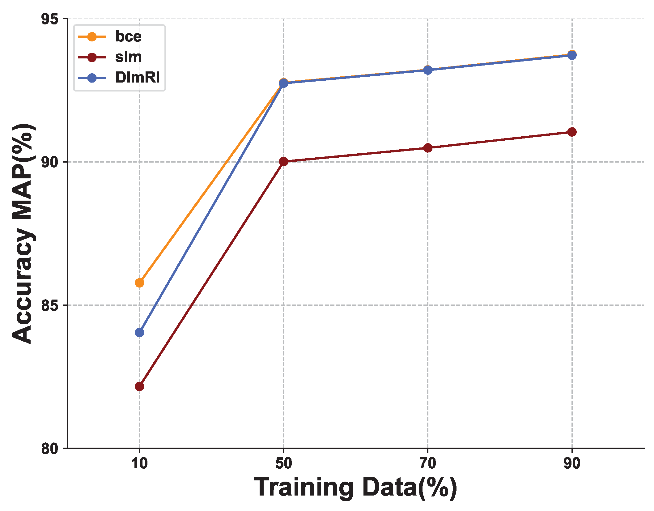
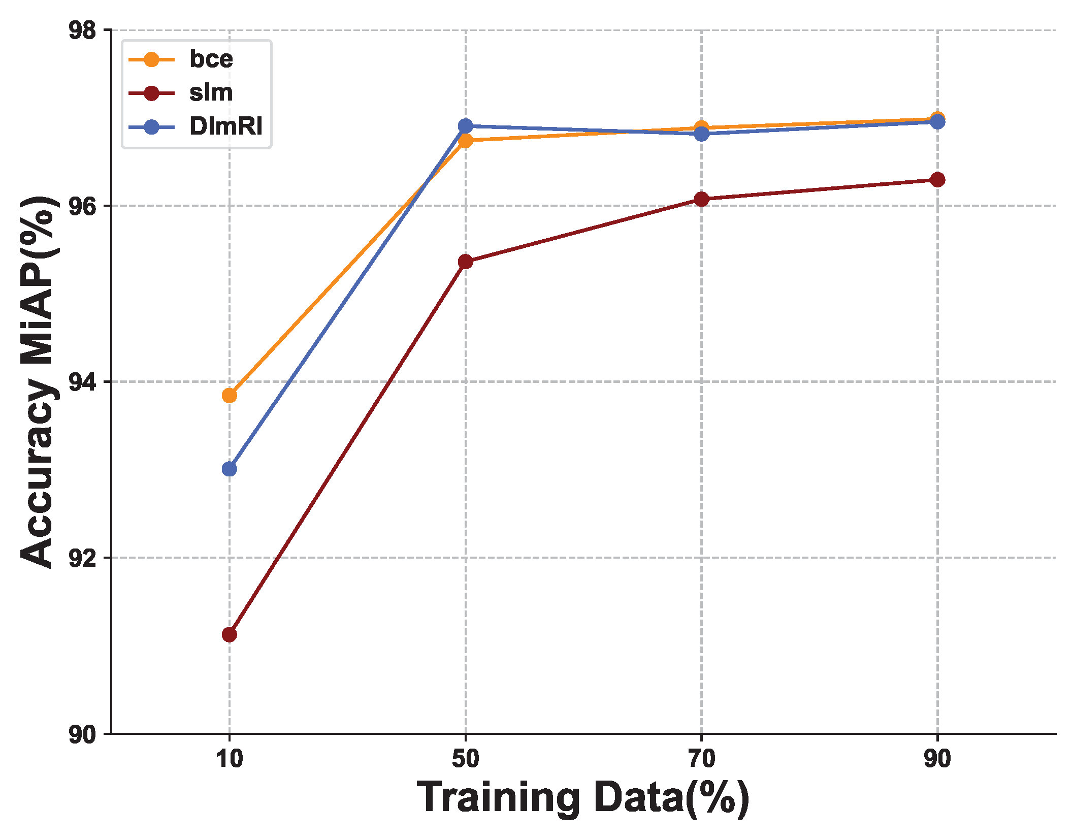
Full labels: We randomly sample a subset of the standard training set for training. The proportion is between $10\%$ ($10\%$ of training images are used) and $100\%$ (all training images are used). The results of ResNet-101 using different loss functions are shown in Figure 2 and Figure 3, from which we can see: (1) as the number of training samples increases, the performance of all models improves gradually; (2) Our method performs slightly worse than the bce method when only 10% of the training data are available, but this can be viewed as the cost of learning more robust feature representations. As the training data increase, the performance of the DlmRl method is able to maintain the highest level, which is due to the fact that the margin plays a lesser role when the amount of data is small than when the amount of data is large, illustrating that our method can effectively improve accuracy when dealing with large-scale data, as it can impose the margin in a large amount of data, which is more advantageous compared to other methods in dealing with large amount of data.

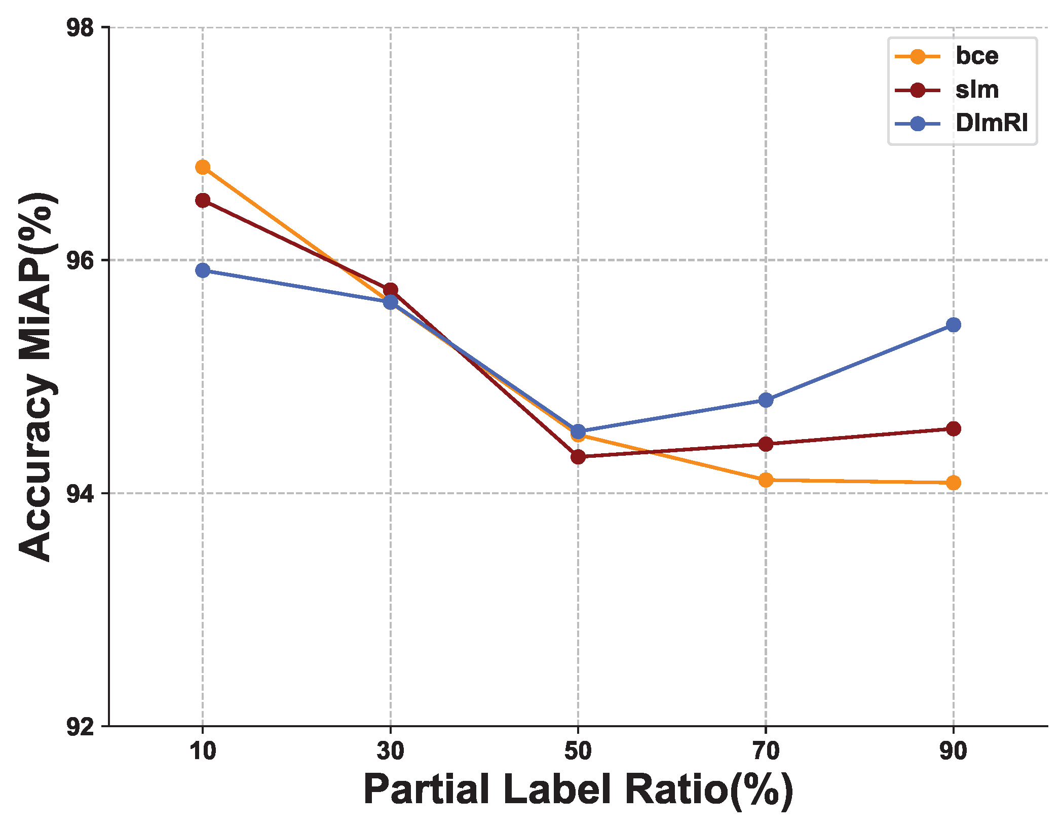
Partial labels: We generate an extreme partial dataset by keeping only one positive label per image. The simulation copes with extreme single-label datasets in reality, e.g., ImageNet. If the image has more than one positive label, we randomly select one positive label among the positive labels and switch the other positive labels to negative labels. The proportion of partial images in the standard training set is between $10\%$ ($10\%$ of training images only have one positive label) and $90\%$ ($90\%$ of the training images only have one positive label). The performances of different loss functions on the partial dataset are shown in Figure 4 and Figure 5, from which we can see that: (i) As the proportion of partial training samples increases, the performance of all loss functions degrade gradually. (ii) The performance of $bce$ loss function drops the fastest and the performance degradation of our loss function is the slowest. (iii) When the fraction exceeds $30\%$, the performance of our loss function is consistently better than other loss functions. This shows that our DlmRl can cope with extreme datasets very well. In a dataset with almost all single labels, our method has an extremely good performance compared to other methods, which shows that DlmRl has excellent robustness in dealing with datasets with sparse labels. Due to the good robustness of DlmRl to extreme datasets, it is possible to only label the main items of the images when labeling them realistically.

Noisy labels: In this experiment, we randomly choose, for each training image, whether to flip its positive/negative label to the other label. The fraction of such flipped labels range from $5\%$ to $20\%$ in increments of $5\%$. An increment of $5\%$ means that the $5\%$ of labels are wrong during training, while $95\%$ of other labels are clean. The performance of different loss functions on the partial dataset are shown in

Table 1. MAP and MiAP score (%) of different methods on VOC2007.

Methods	Noisy Ratio 5%	Noisy Ratio 10%	Noisy Ratio 15%	Noisy Ratio 20%
bce (MAP) [31]	88.79	85.50	82.83	80.05
slm (MAP) [41]	88.70	85.48	83.13	79.96
DlmRl (MAP)	90.77	90.57	90.24	89.90
bce (MiAP) [31]	94.74	93.28	91.69	89.82
slm (MiAP) [41]	94.70	93.19	91.68	89.94
DlmRl (MiAP)	95.96	95.68	95.00	94.77

, Compared with bce, we observe a substantial improvement in the MAP of 1.98%, 5.07%, 7.41% and 9.85% for the 5%, 10%, 15% and 20% ratio of noisy labels, respectively. from which we can see that: (i) Under all noise ratios, DlmRl is consistently more robust than other methods. (ii) As the noise ratio increases, the performance of DlmRl only slightly decreases. (iii) As the noise ratio increases, the performance of slm degrades the fastest, which reveals the limitation of the traditional large-margin technique.

4.3. Results on MS-COCO Dataset

MS-COCO Microsoft is widely used for segmentation, classification, detection and captioning. We use COCO-2014 in our experiments, which has 82,081 training images and 40,137 validation images and 80 object classes. Due to the large scale of this dataset, we conduct only one experiment for each of the three labeled scenarios, i.e., full label, partial label and noisy label. The ratios in the full, partial and noisy label scenarios are randomly set to 10%, 10% and 5%, respectively. From

Table 2. MAP and MiAP score (%) of different methods on MS-COCO.

Methods	Training Ratio 10%	Particle Ratio 10%	Noisy Ratio 5%
bce (MAP) [31]	65.53	74.16	75.90
slm (MAP) [41]	65.29	74.21	75.87
DlmRl (MAP)	65.25	74.83	75.99
bce (MiAP) [31]	84.12	87.00	88.11
slm (MiAP) [41]	84.05	87.10	88.03
DlmRl (MiAP)	84.12	87.68	88.15

, we can see that DlmRl can achieve comparable performance against its counterparts on the full labels scenario, but significantly better performance than them on the partial and noisy label scenarios.

4.4. Ablation Study

In this subsection, we conduct experiments to study the effect of different hyper-parameters or components of our loss function on the VOC2007 dataset. To discuss the effect of one hyper-parameter, we conduct experiments on its different values, but keep other hyper-parameters or components fixed.

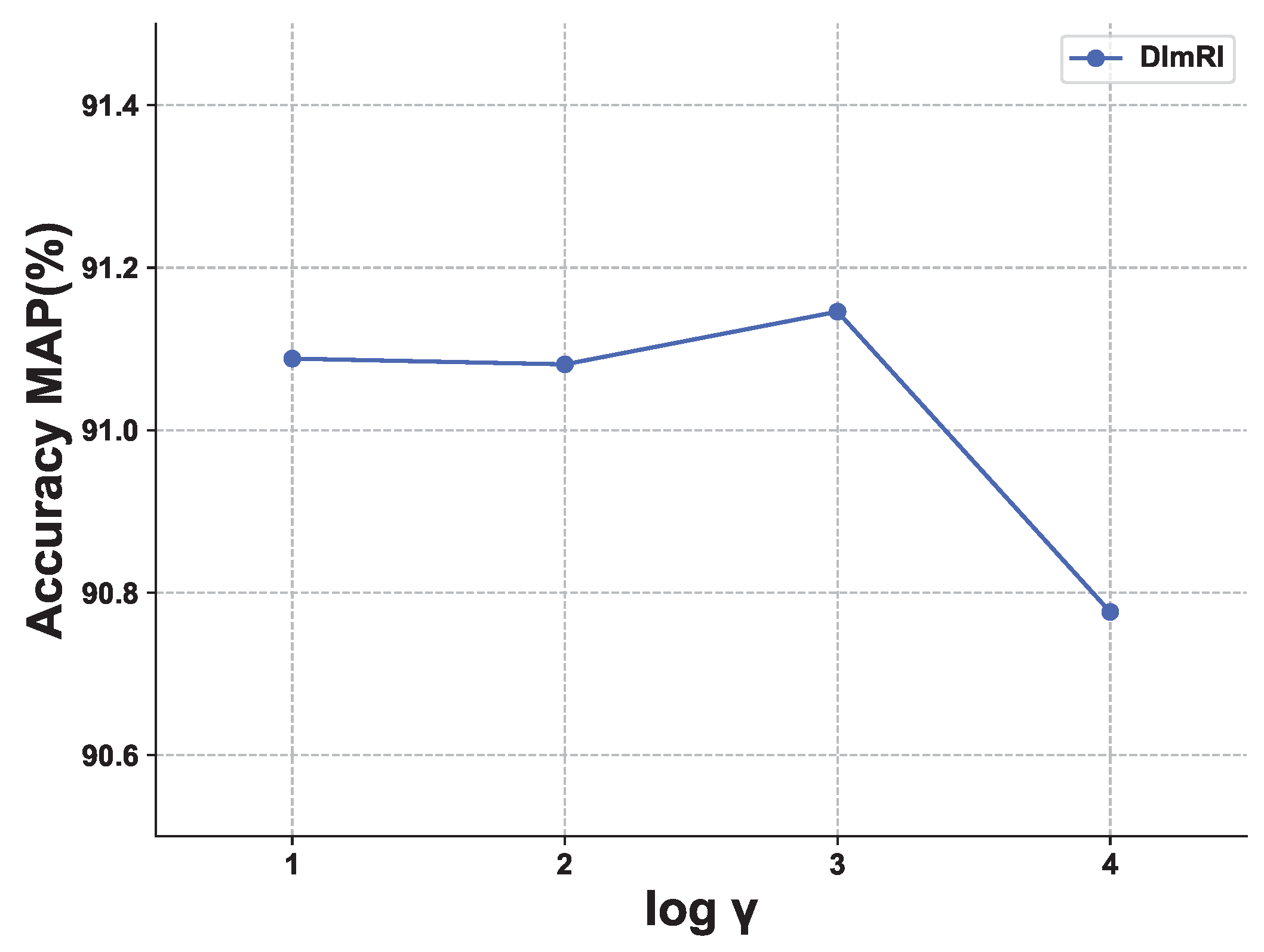
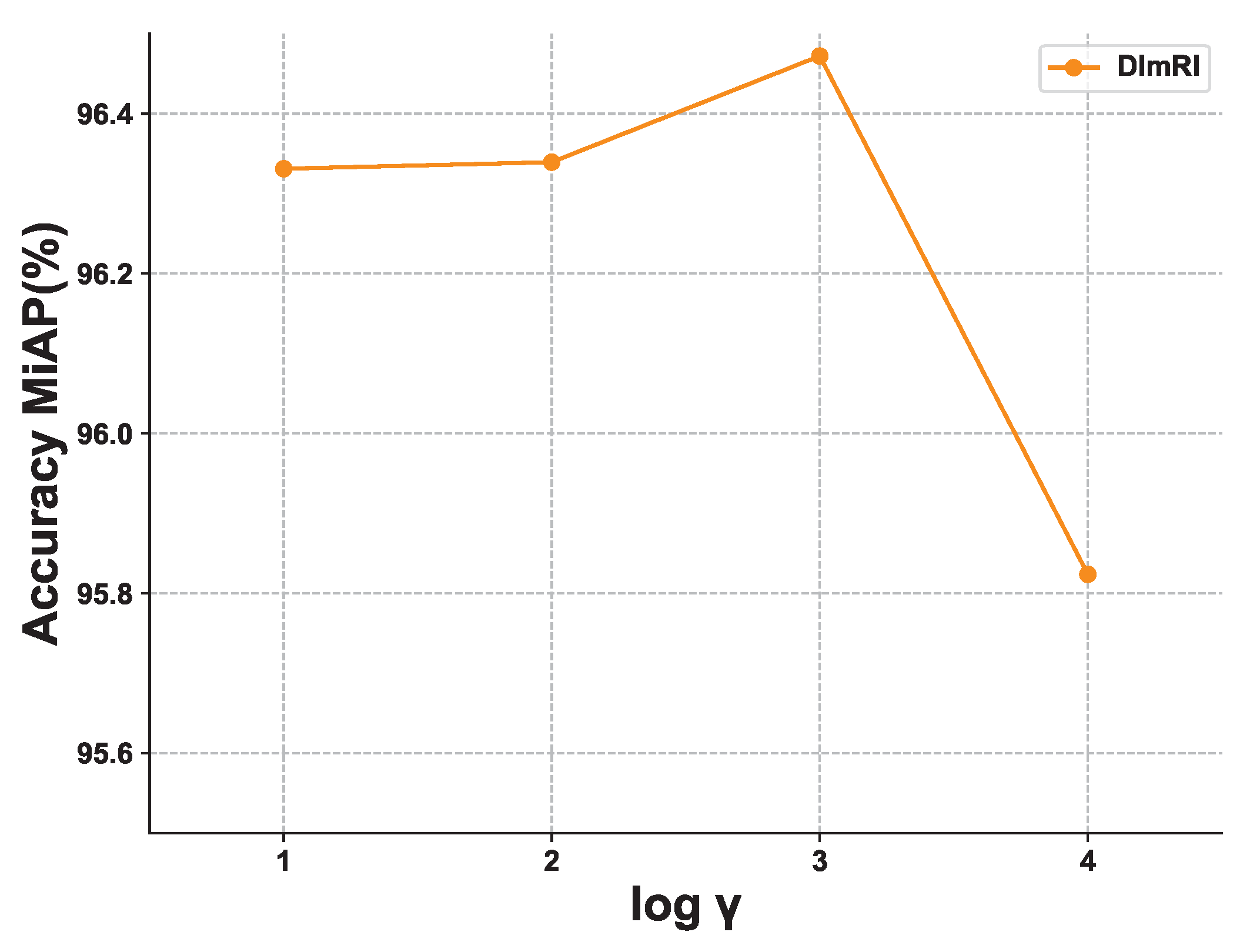
Figure 6 and Figure 7 show the effect of $\gamma$ with values in $\{{10}^1,{10}^2,{10}^3,{10}^4\}$. The penalty includes the distance that $I^k$ needs to travel to reach the ranking threshold as well as another $\gamma$ distance to travel on the correct side of the ranking threshold to attain the $\gamma$ margin. As can be seen, the performance of different values is very similar, so the classification performance is not very sensitive to $\gamma$.

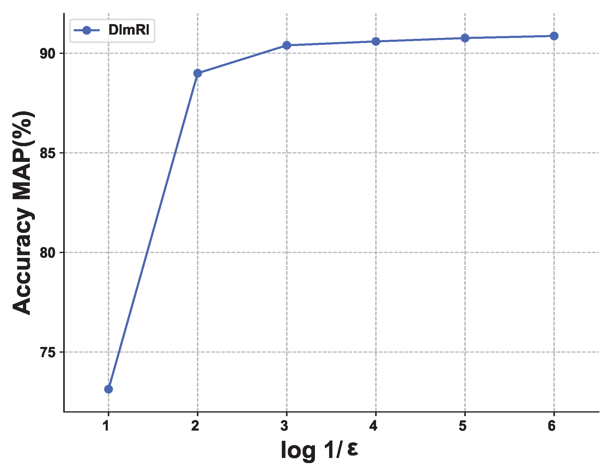
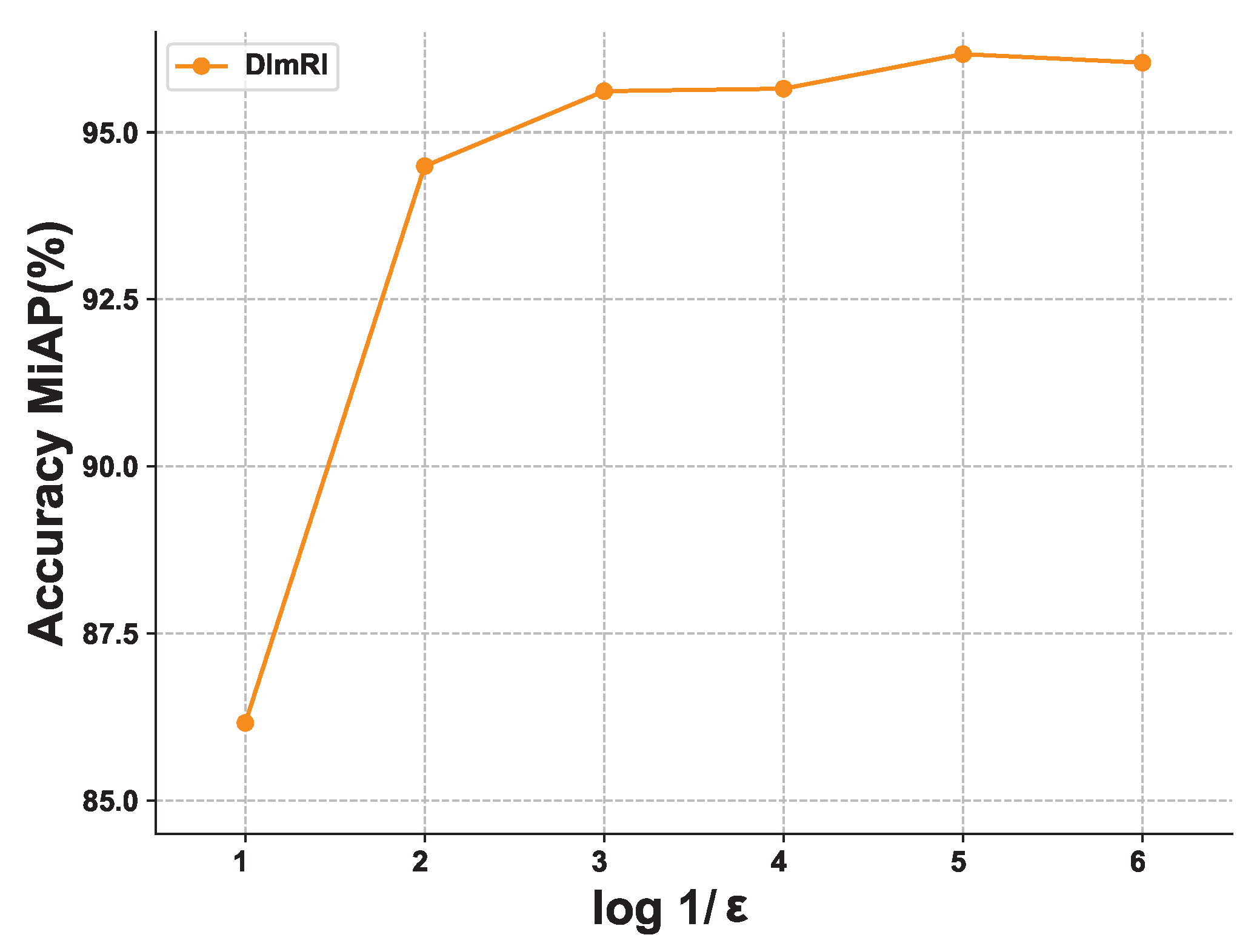
Figure 8 and Figure 9 show the effect of $ϵ$ with values in $\{{10}^{-1},{10}^{-2},\dots ,{10}^{-6}\}$. As can be seen, a small value of $ϵ$ is very important. When the value is small enough, the classification performance will only change slightly. The $ϵ$ is used to prevent numerical problems. This experimental result is reasonable. When the value of $\mathsf{\epsilon }$ is too small, the maximum margin represented by Formula (12) will be too large, and when it exceeds a certain range, the effect of our DlmRl will not be displayed.

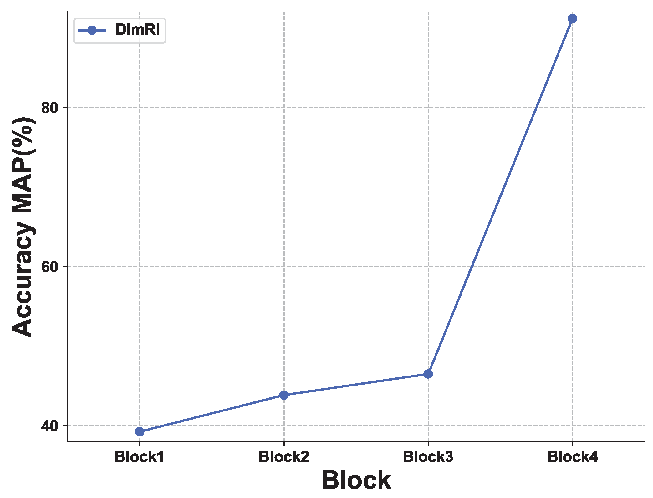
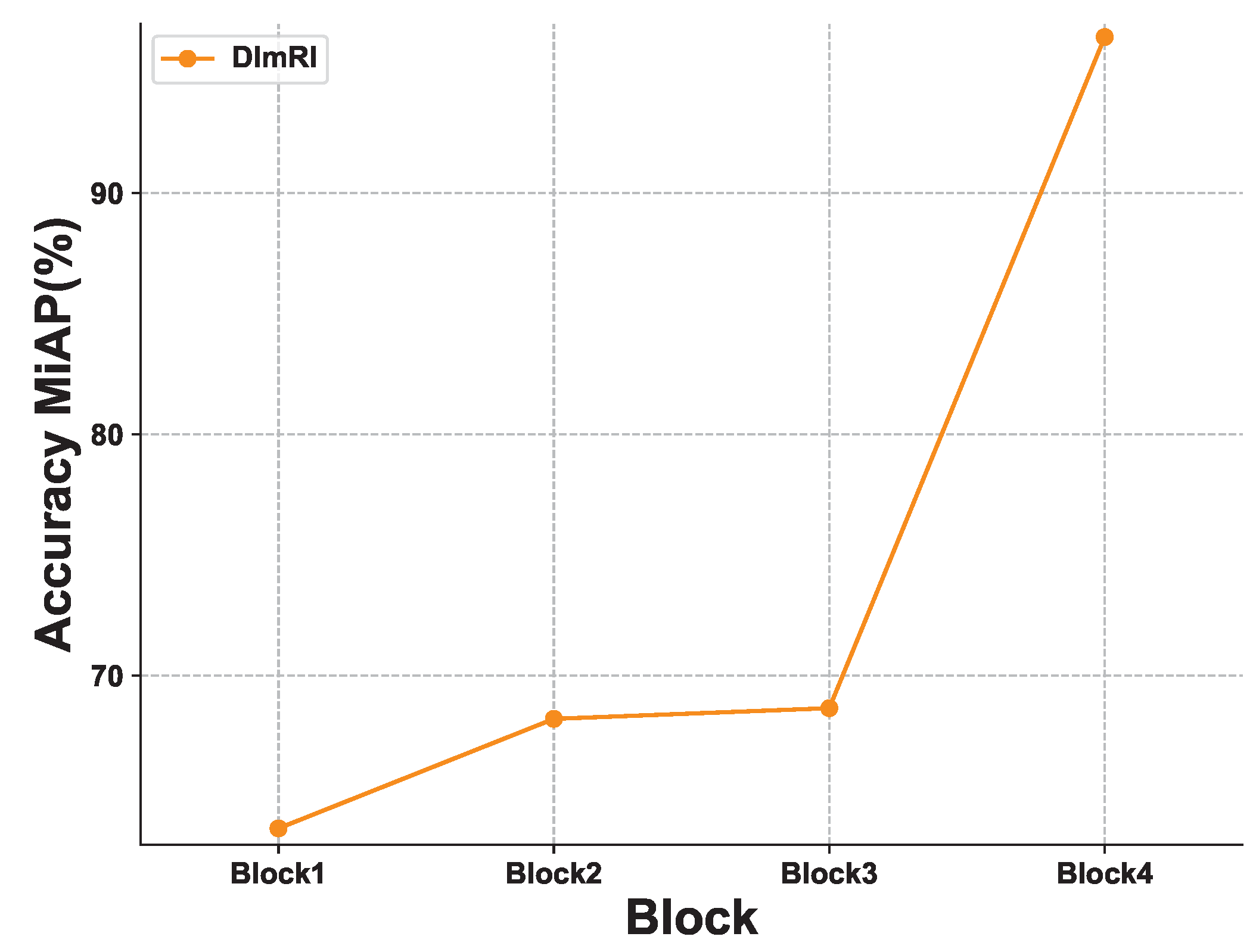
The architecture of ResNet-101 consists of four blocks from bottom to up, i.e., Block1, Block2, Block3 and Block4, as well as two fully connected layers. To analyze the effect of imposing a margin on different hidden neural network layers, we conduct experiments on the four different blocks of ResNet-101, respectively. Figure 10 and Figure 11 show the experimental results. As can be seen, it achieves the best MAP score and MiAP score by imposing a margin on Block4.

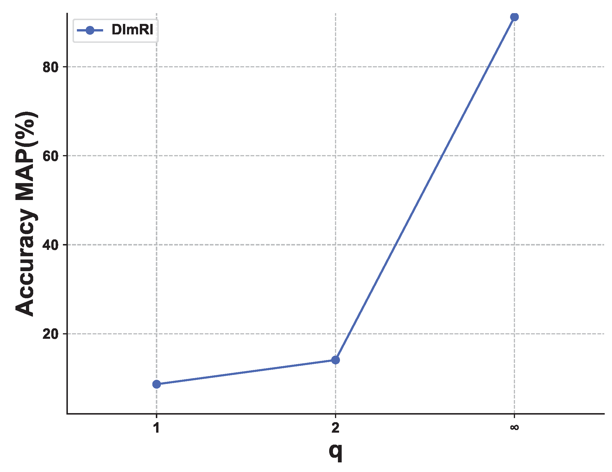
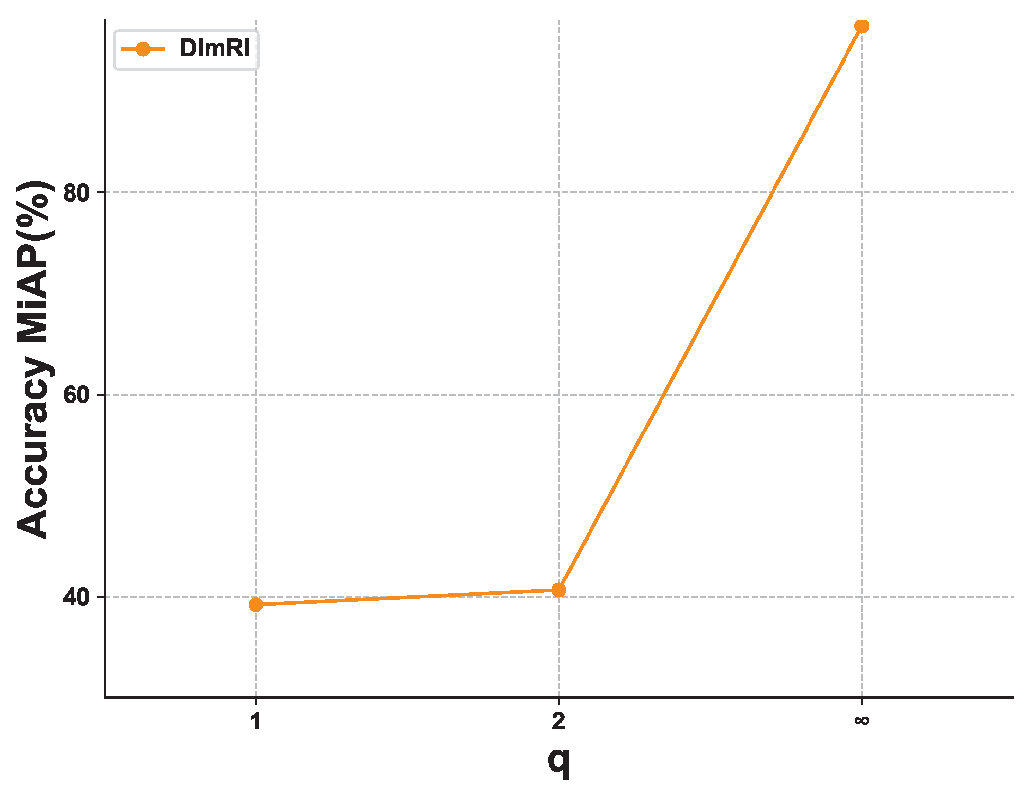
Figure 12 and Figure 13 show the effect of q with values in $\{1,2,\infty \}$. As can be seen, the classification performance is sensitive to this parameter and $q=\infty$ is the best.

According to the above analysis, in the experiments described previously, we set $\gamma ={10}^3, ϵ={10}^{-6}, q=\infty$ and impose large margin on Block4 of ResNet-101 by default.

5. Conclusions

In this paper, we have proposed a novel loss, i.e., DlmRl, for a MLiC task. It is a plug and play loss, and is thus applicable to any network architecture. In contrast to a traditional large margin, the ranking loss encourages only margins at the output layer of a deep neural network, so the proposed loss formulation imposes a margin on any chosen set of layers of a deep network and allows choosing any ${\ell }_p$ norm ($p\ge 1$) on the metric measuring the margin between labels— showing a far more flexible and compatible implementation. We design a negative sampling technique to make it more computationally efficient, thus addressing the scalability issues brought by full computation. Experiments on the VOC2007 dataset and the COCO dataset have verified that our DlmRl is better than other methods by applying a margin to the input layer, and our computational efficiency has been greatly improved thanks to the introduction of negative sampling technology. Extensive experiments show that our loss formulation is more robust than traditional loss formulations of MLiC.

References

1. Chen, L.; Zhan, W.; Tian, W.; He, Y.; Zou, Q. Deep integration: A multi-label architecture for road scene recognition. IEEE Trans. Image Process. 2019, 28, 4883–4898. [Google Scholar] [CrossRef] [PubMed]
2. Chen, B.; Zhang, Z.; Lu, Y.; Chen, F.; Lu, G.; Zhang, D. Semantic-interactive graph convolutional network for multilabel image recognition. IEEE Trans. Syst. Man Cybern. Syst. 2021, 52, 4887–4899. [Google Scholar] [CrossRef]
3. Ge, Z.; Mahapatra, D.; Sedai, S.; Garnavi, R.; Chakravorty, R. Chest x-rays classification: A multi-label and fine-grained problem. arXiv 2018, arXiv:1807.07247. [Google Scholar]
4. Gérardin, C.; Wajsbürt, P.; Vaillant, P.; Bellamine, A.; Carrat, F.; Tannier, X. Multilabel classification of medical concepts for patient clinical profile identification. Artif. Intell. Med. 2022, 128, 102311. [Google Scholar] [CrossRef] [PubMed]
5. Boutell, M.R.; Luo, J.; Shen, X.; Brown, C.M. Learning multi-label scene classification. Pattern Recognit. 2004, 37, 1757–1771. [Google Scholar] [CrossRef] [Green Version]
6. Tsoumakas, G.; Vlahavas, I. Random k-labelsets: An ensemble method for multilabel classification. In European Conference on Machine Learning; Springer: Berlin/Heidelberg, Germany, 2007; pp. 406–417. [Google Scholar]
7. Zhang, M.L.; Zhou, Z.H. Ml-knn: A lazy learning approach to multi-label learning. Pattern Recognit. 2007, 40, 2038–2048. [Google Scholar] [CrossRef] [Green Version]
8. Elisseeff, A.; Weston, J. A kernel method for multi-labelled classification. Adv. Neural Inf. Process. Syst. 2001, 14, 681–687. [Google Scholar]
9. Lowe, D.G. Distinctive image features from scaleinvariant keypoints. Int. J. Comput. Vis. 2004, 60, 91–110. [Google Scholar] [CrossRef]
10. Dalal, N.; Triggs, B. Histograms of oriented gradients for human detection. In Proceedings of the 2005 IEEE Computer Society Conference on Computer Vision and Pattern Recognition (CVPR’05), San Diego, CA, USA, 20–26 June 2005; IEEE: Piscataway, NJ, USA, 2005; Volume 1, pp. 886–893. [Google Scholar]
11. Ojala, T.; Pietikäinen, M.; Harwood, D. A comparative study of texture measures with classification based on featured distributions. Pattern Recognit. 1996, 29, 51–59. [Google Scholar] [CrossRef]
12. Wang, J.; Yang, Y.; Mao, J.; Huang, Z.; Huang, C.; Xu, W. Cnn-rnn: A unified framework for multi-label image classification. In Proceedings of the IEEE Conference on Computer Vision and Pattern Recognition, Las Vegas, NV, USA, 27–30 June 2016; pp. 2285–2294. [Google Scholar]
13. Chen, Z.M.; Wei, X.S.; Wang, P.; Guo, Y. Multi-label image recognition with graph convolutional networks. In Proceedings of the IEEE/CVF Conference on Computer Vision and Pattern Recognition, Long Beach, CA, USA, 15–20 June 2019; pp. 5177–5186. [Google Scholar]
14. Xu, Z.; Liu, Y.; Li, C. Distributed information-theoretic semisupervised learning for multilabel classification. IEEE Trans. Cybern. 2022, 52, 821–835. [Google Scholar] [CrossRef]
15. Ma, J.; Chiu, B.C.Y.; Chow, T.W.S. Multilabel classification with group-based mapping: A framework with local feature selection and local label correlation. IEEE Trans. Cybern. 2020, 52, 4596–4610. [Google Scholar] [CrossRef]
16. Elsayed, G.; Krishnan, D.; Mobahi, H.; Regan, K.; Bengio, S. Large margin deep networks for classification. Adv. Neural Inf. Process. Syst. 2018, 31, 842–852. [Google Scholar]
17. Chen, L.; Wang, R.; Yang, J.; Xue, L.; Hu, M. Multi-label image classification with recurrently learning semantic dependencies. Vis. Comput. 2019, 35, 1361–1371. [Google Scholar] [CrossRef]
18. Liu, F.; Xiang, T.; Hospedales, T.M.; Yang, W.; Sun, C. Semantic regularisation for recurrent image annotation. In Proceedings of the IEEE Conference on Computer Vision and Pattern Recognition, Honolulu, HI, USA, 21–26 July 2017; pp. 2872–2880. [Google Scholar]
19. Meng, Q.; Zhang, W. Multilabel image classification with attention mechanism and graph convolutional networks. In Proceedings of the ACM Multimedia Asia, Beijing, China, 16–18 December 2019; pp. 1–6. [Google Scholar]
20. Wu, X.; Chen, Q.; Li, W.; Xiao, Y.; Hu, B. Adahgnn: Adaptive hypergraph neural networks for multi-label image classification. In Proceedings of the 28th ACM International Conference on Multimedia, Seattle, WA, USA, 12–16 October 2020; pp. 284–293. [Google Scholar]
21. Oquab, M.; Bottou, L.; Laptev, I.; Sivic, J. Is object localization for free?-weakly-supervised learning with convolutional neural networks. In Proceedings of the IEEE Conference on Computer Vision and Pattern Recognition, Boston, MA, USA, 7–12 June 2015; pp. 685–694. [Google Scholar]
22. Gou, J.; Sun, L.; Du, L.; Ma, H.; Xiong, T.; Ou, W.; Zhan, Y. A representation coefficient-based k-nearest centroid neighbor classifier. Expert Syst. Appl. 2022, 194, 116529. [Google Scholar] [CrossRef]
23. Zhou, B.; Khosla, A.; Lapedriza, A.; Oliva, A.; Torralba, A. Learning deep features for discriminative localization. In Proceedings of the IEEE Conference on Computer Vision and Pattern Recognition, Las Vegas, NV, USA, 27–30 June 2016; pp. 2921–2929. [Google Scholar]
24. Martins, A.; Astudillo, R. From softmax to sparsemax: A sparse model of attention and multilabel classification. In Proceedings of the International Conference on Machine Learning (PMLR 2016), New York, NY, USA, 19–24 June 2016; pp. 1614–1623. [Google Scholar]
25. Zhu, K.; Wu, J. Residual attention: A simple but effective method for multi-label recognition. In Proceedings of the IEEE/CVF International Conference on Computer Vision, Montreal, QC, Canada, 10–17 October 2021; pp. 184–193. [Google Scholar]
26. Ma, Z.; Chen, S. A Similarity-based Framework for Classification Task. IEEE Trans. Knowl. Data Eng. 2022. [Google Scholar] [CrossRef]
27. Izadinia, H.; Russell, B.C.; Farhadi, A.; Hoffman, M.D.; Hertzmann, A. Deep classifiers from image tags in the wild. In Proceedings of the 2015 Workshop on Community-Organized Multimodal Mining: Opportunities for Novel Solutions, Brisbane, Australia, 26–30 October 2015; pp. 13–18. [Google Scholar]
28. Xie, M.K.; Huang, S.J. Partial multi-label learning with noisy label identification. IEEE Trans. Pattern Anal. Mach. Intell. 2021, 44, 3676–3689. [Google Scholar] [CrossRef]
29. Durand, T.; Mehrasa, N.; Mori, G. Learning a deep convnet for multi-label classification with partial labels. In Proceedings of the IEEE/CVF Conference on Computer Vision and Pattern Recognition, Long Beach, CA, USA, 15–20 June 2019; pp. 647–657. [Google Scholar]
30. Huynh, D.; Elhamifar, E. Interactive multi-label cnn learning with partial labels. In Proceedings of the IEEE/CVF Conference on Computer Vision and Pattern Recognition, Seattle, WA, USA, 13–19 June 2020; pp. 9423–9432. [Google Scholar]
31. Gong, Y.; Jia, Y.; Leung, T.; Toshev, A.; Ioffe, S. Deep convolutional ranking for multilabel image annotation. arXiv 2013, arXiv:1312.4894. [Google Scholar]
32. Cortes, C.; Vapnik, V. Support-vector networks. Mach. Learn. 1995, 20, 273–297. [Google Scholar] [CrossRef]
33. Freund, Y.; Schapire, R.E. A decision-theoretic generalization of on-line learning and an application to boosting. J. Comput. Syst. Sci. 1997, 55, 119–139. [Google Scholar] [CrossRef] [Green Version]
34. Sun, S.; Chen, W.; Wang, L.; Liu, T.-Y. Large margin deep neural networks: Theory and algorithms. arXiv 2015, arXiv:1506.05232. [Google Scholar]
35. Sokolić, J.; Giryes, R.; Sapiro, G.; Rodrigues, M.R.D. Robust large margin deep neural networks. IEEE Trans. Signal Process. 2017, 65, 4265–4280. [Google Scholar] [CrossRef]
36. Li, Y.; Song, Y.; Luo, J. Improving pairwise ranking for multi-label image classification. In Proceedings of the IEEE Conference on Computer Vision and Pattern Recognition, Honolulu, HI, USA, 21–26 July 2017; pp. 3617–3625. [Google Scholar]
37. Everingham, M.; Eslami, S.M.; Van Gool, L.; Williams, C.K.; Winn, J.; Zisserman, A. The pascal visual object classes challenge: A retrospective. Int. J. Comput. Vis. 2015, 111, 98–136. [Google Scholar] [CrossRef]
38. Lin, T.Y.; Maire, M.; Belongie, S.; Hays, J.; Perona, P.; Ramanan, D.; Dollár, P.; Zitnick, C.L. Microsoft coco: Common objects in context. In European Conference on Computer Vision; Springer: Cham, Switzerland, 2014; pp. 740–755. [Google Scholar]
39. Baeza-Yates, R.; Ribeiro-Neto, B. Modern Information Retrieval; ACM Press: New York, NY, USA, 1999; Volume 463. [Google Scholar]
40. Xie, M.K.; Huang, S.J. Ccmn: A general framework for learning with class-conditional multi-label noise. IEEE Trans. Pattern Anal. Mach. Intell. 2022. [Google Scholar] [CrossRef] [PubMed]
41. Imambi, S.; Prakash, K.B.; Kanagachidambaresan, G.R. PyTorch. In Programming with TensorFlow; Springer: Cham, Switzerland, 2021; pp. 87–104. [Google Scholar]
Figure 1. As shown in the above figure, the left side represents the prediction value of image ( I k ) obtained through the prediction model, and the right side represents the predicted value of the image with perturbations ( I k + δ ) obtained through the prediction model. The positive labels in the clean image include: umbrella, rain coat, car and person; negative labels include trunk and sunglasses. We hope that our model is robust to perturbations I k + δ . For example, the car is the positive label in the real predicted value. After the perturbations are added, the predicted value of the car is still higher than that of negative labels.
Mathematics 10 04584 g001
Figure 2. The figure shows the MAP score (%) of three different loss methods on VOC2007 with full labels. The orange line indicates the accuracy rate using BCE with Logits Loss (bce): the red line indicates the accuracy rate using MultiLabel SoftMargin Loss (slm); and the blue line indicates the accuracy rate using our DlmRl.
Mathematics 10 04584 g002
Figure 3. The figure shows the MiAP score (%) of three different loss methods on VOC2007 with full labels. The orange line indicates the accuracy rate using BCE with Logits Loss (bce); the red line indicates the accuracy rate using MultiLabel SoftMargin Loss (slm); and the blue line indicates the accuracy rate using our DlmRl.
Mathematics 10 04584 g003
Figure 4. The figure shows the MAP score (%) of three different loss methods on VOC2007 with partial labels. The orange line indicates the accuracy rate using BCE with Logits Loss (bce): the red line indicates the accuracy rate using MultiLabel SoftMargin Loss (slm); and the blue line indicates the accuracy rate using our DlmRl.
Mathematics 10 04584 g004
Figure 5. The figure shows the MiAP score (%) of three different loss methods on VOC2007 with partial labels. The orange line indicates the accuracy rate using BCE with Logits Loss (bce): the red line indicates the accuracy rate using MultiLabel SoftMargin Loss (slm); and the blue line indicates the accuracy rate using our DlmRl.
Mathematics 10 04584 g005
Figure 6. The figure shows the effect of γ on the MAP score using our DlmRl.
Mathematics 10 04584 g006
Figure 7. The figure shows the effect of γ on the MiAP score using our DlmRl.
Mathematics 10 04584 g007
Figure 8. The figure shows the effect of ϵ on the MAP score using our DlmRl.
Mathematics 10 04584 g008
Figure 9. The figure shows the effect of ϵ on the MiAP score using our DlmRl.
Mathematics 10 04584 g009
Figure 10. The figure shows the effect of imposing a margin on different blocks on the MAP score using our DlmRl.
Mathematics 10 04584 g010
Figure 11. The figure shows the effect of imposing a margin on different blocks on the MiAP score using our DlmRl.
Mathematics 10 04584 g011
Figure 12. The figure shows the effect of q on the MAP score using our DlmRl.
Mathematics 10 04584 g012
Figure 13. The figure shows the effect of q about MiAP score which using our DlmRl.
Mathematics 10 04584 g013