Analytical and Numerical Study on Forced and Damped Complex Duffing Oscillators

Abstract

In this work, some general forms for forced and damped complex Duffing oscillators (FDCDOs), including two different models, which are known as the forced and damped complex Duffing oscillator (I) (FDCDO (I)) and FDCDO (II), are investigated by using some effective analytical and numerical approaches. For the analytical approximation, the two models of the FDCDOs are reduced to two decoupled standard forced and damped Duffing oscillators (FDDOs). After that, both the ansatz method and Krylov–Bogoliubov–Mitropolsky (KBM) approach are applied in order to derive some accurate analytical approximations in terms of trigonometric functions. For the numerical approximations, the finite difference method is employed to analyze the two coupled models without causing them to be decoupled for the original problems. In addition, all obtained analytical and numerical approximations are compared with the fourth-order Runge–Kutta (RK4) numerical approximations. Moreover, the maximum residual distance error (MRDE) is estimated in order to verify the accuracy of all obtained approximations.

1. Introduction

Nonlinear oscillation is one of the most popular and widely researched fields due to its diverse applications in automobiles, sensing, fluid and solid interactions, bioengineering, and plasma oscillations [1,2,3,4,5,6,7,8]. There are huge numbers of equations of motion that can be used to model and describe the mechanisms of motion of various waves and oscillators [9,10]. For instance, Cveticanin [1,2] used the hybrid elliptic-Krylov–Bogolubov method (eKBM) with the power-series method (PSM) to analyze a conserved coupled system of second-order differential equations (DEs) with weak and strong nonlinearity. In [1], the author used the mentioned method to derive only the first-order approximation in terms of Jacobi elliptic functions (JEFs). In addition, Cveticanin [2] used the eKBM to derive some analytical approximations in terms of JEFs for strong nonlinear DEs of complex Duffing-type oscillators, which describe the dynamical behavior of numerous realistic models. Grattarola and Torre [4] derived the sufficient and necessary conditions for synchronization, which can be applied in order to find much information about a wide range of nonlinear oscillators. Cveticanin [5] presented an approximate technique based on a method of slowly varying the phase and amplitude in order to solve a set of two coupled complex ordinary differential equations (ODEs). Mahmoud [6] used an approximate method based on the Krylov–Bogoliubov averaging approach to analyze and solve a set of complex nonlinear physical oscillators. Manasevich et al. [7] studied complex-valued Liénard systems to obtain the sufficient conditions for periodic solutions to these issues. Cveticanin [8] used the averaging method to derive an exact solution to a cubic-nonlinearity complex differential equation in terms of JEFs. Moreover, nonlinear plasma oscillations were analyzed in the framework of a general form of the Van der Pol oscillator [9]. The authors of [9] used some effective approximate methods, such as the ansatz method and the Krylov–Bogoliubov–Mitropolsky (KBM) method, to derive some analytic approximations. Both the equivalent linearization approach (ELA) and weighted averaging were employed [11,12] to analyze many different types of strong nonlinear oscillators, including many different Duffing-type oscillators and a cubic Duffing oscillator with discontinuity. The authors compared their results with those of many other approaches, such as the min–max approach, the parameter-expansion method, the modified Lindsted–Poincare method, the homotopy perturbation method, and the fourth-order Runge–Kutta (RK4) numerical method. Hieu [13] used the ELP with weighted averaging to derive an approximation to a generalized strong nonlinear oscillator with a fractional term. As a special case for the obtained results, the author of [13] studied the approximations to some different types of Duffing oscillators and a nonlinear oscillator with fractional nonlinearity. In addition, this author compared his results with those of RK4 numerical approximations.

The Duffing-type equation/oscillator is one of the most famous and important equations, as it has succeeded in explaining many different oscillations in different plasma oscillations [14], engineering problems [15], statistical mechanics, and many other applications [16,17,18]. Moreover, there is another form of the Duffing equation with complex variables, which is known as a complex Duffing oscillator (CDO) [1,2], as mentioned above. One of these equations was studied in [1] by Cveticanin, who solved the following problem:

$$\left\{\begin{array}{c}\ddot{x}+m{x}^3-y=ϵF_1\left(x,\dot{x},y,\dot{y}\right),\\ \ddot{y}-p{x}^5-ax=ϵF_2\left(x,\dot{x},y,\dot{y}\right),\\ x\left(0\right)=x_0\& \dot{x}\left(0\right)={\dot{x}}_0,\\ y\left(0\right)=x_0\& \dot{y}\left(0\right)={\dot{y}}_0.\end{array}\right.$$

(1)

Here, $F_1\equiv F_1\left(x,\dot{x},y,\dot{y}\right)$ and $F_2\equiv F_2\left(x,\dot{x},y,\dot{y}\right)$ are weakly nonlinear functions, and $\left(a,m,p\right)$ are the parameters of the model under study. In addition, Cveticanin [2] analyzed and discussed the following complex Duffing-type oscillator:

$$\ddot{z}+c_{1}z+3c_{3}z{\left|z\right|}^2-c_3{\overline{z}}^3=ϵG\left(z,\dot{z},cc\right),$$

(2)

where $z\equiv z\left(t\right)$, $x\left(t\right)\equiv x$, $y\left(t\right)\equiv y$, $z\equiv x+iy$ is a complex function, and $\overline{z}$ is the conjugate of z, whereas $x\equiv x\left(t\right)$ and $y\equiv y\left(t\right)$ indicate the real and imaginary parts, respectively. $z\overline{z}={\left|z\right|}^2$, $G\left(z,\dot{z},cc\right)$ represents a complex defection, “$cc$”indicates the complex conjugate function, and $i=\sqrt{-1}$. In [3], the authors investigated a cubic DE and presented the desired solutions in different forms of functions, such as Jacobi and Weierstrass elliptic functions. In the present investigation, the following two general forms of the forced damped CDO are considered:

$$\ddot{z}+2\epsilon \dot{z}+\alpha z+\beta z{\left|z\right|}^2+\gamma {\overline{z}}^3=ϝ\left(t\right),$$

(3)

and

$$\ddot{z}+2\epsilon \dot{z}+\alpha z+\tilde{\beta }z{\left|z\right|}^2+\tilde{\gamma }{\overline{z}}^3+\tilde{\delta }{z}^3=ϝ\left(t\right),$$

(4)

where $ϝ\left(t\right)=f_1\left(t\right)+i{f}_2\left(t\right)$ indicates any periodic force that can be taken as $f_1\left(t\right)={\gamma }_{1}cos\left({\omega }_{1}t\right)$ and $f_2\left(t\right)={\gamma }_{2}cos\left({\omega }_{2}t\right)$ or any other time-dependent function. The coefficients $\left(\epsilon ,\alpha ,\beta ,\gamma \right)$ of Equation (3) are real values, while for Equation (4), the coefficients $\left(\epsilon ,\alpha ,\right)$ are real values, but $\left(\tilde{\beta },\tilde{\gamma },\tilde{\delta }\right)$ have complex values, as follows:

$$\left\{\begin{array}{c}\tilde{\beta }=({\beta }_1+i{\beta }_2),\\ \tilde{\gamma }=({\gamma }_1+i{\gamma }_2),\\ \tilde{\delta }=({\delta }_1+i{\delta }_2).\end{array}\right.$$

(5)

In this investigation, two different models for the forced damped CDO, including the FDCDO (I) (3) and the FDCDO (II) (4), will be analyzed and discussed by using some effective techniques, such as the ansatz method, KBM approach [19], and finite difference method (FDM). The two mentioned models are analyzed by using both the ansatz method and the KBM approach in order to find some analytic approximations in terms of trigonometric functions. To do that, the two aforementioned models will be reduced to two decoupled systems of standard forced and damped Duffing oscillators (FDDOs). After that, both the ansatz and KBM methods can be applied in order to find some analytical approximations to the standard forced and damped Duffing oscillator (FDDO). However, for the numerical approximations, both the FDM and RK4 methods will be applied in order to analyze and solve the original complex problems numerically without causing them to be decoupled from the original problems.

2. FDCDO (I)

Let us consider the following initial value problem (i.v.p.):

$$\left\{\begin{array}{c}\ddot{z}+2\epsilon \dot{z}+\alpha z+\beta z{\left|z\right|}^2+\gamma {\overline{z}}^3=ϝ\left(t\right),\\ z\left(0\right)=z_0\& \dot{z}\left(0\right)={\dot{z}}_0,\end{array}\right.$$

(6)

where the coefficients $\left(\epsilon ,\alpha ,\beta ,\gamma \right)$ are real constants and $\alpha >0$. To analyze this system, it should be reduced to two decoupled forced and damped Duffing oscillators (FDDOs) by using a suitable linear transformation.

Reducing the I.V.P. (6) to Two Decoupled FDDOs

Using the relation $z=x+iy$ in the i.v.p. (6), the $x-y$ system is obtained as follows:

$$\left\{\begin{array}{c}{\mathbb{Q}}_1\equiv \ddot{x}+2\epsilon \dot{x}+\alpha x+(\beta +\gamma )x^3+(\beta -3\gamma )y^{2}x-f_1\left(t\right)=0,\\ {\mathbb{Q}}_2\equiv \ddot{y}+2\epsilon \dot{y}+\alpha y+(\beta +\gamma )y^3+(\beta -3\gamma )x^{2}y-f_2\left(t\right)=0,\\ x\left(0\right)=x_0\& y\left(0\right)=y_0,\\ \dot{x}\left(0\right)={\dot{x}}_0\& \dot{y}\left(0\right)={\dot{y}}_0.\end{array}\right.$$

(7)

Note that ${\mathbb{Q}}_{1,2}$ are linearly decoupled, and the following linear transformation can be used to reduce the coupled Equation (7) to two decoupled FDDOs:

$$\left\{\begin{array}{c}x=u+v,\\ y=u-v,\end{array}\right.$$

(8)

where $u\equiv u\left(t\right)$ and $v\equiv v\left(t\right)$ obey the following FDDOs:

$$\left\{\begin{array}{c}\ddot{u}+2{\delta }_1\dot{u}+P_{1}u+Q_1{u}^3=F_1\left(t\right),\\ \ddot{v}+2{\delta }_2\dot{v}+P_{2}v+Q_2{v}^3=F_2\left(t\right).\end{array}\right.$$

(9)

Inserting Equations (8) and (9) into the i.v.p. (7), after several calculations, the following values of the coefficients ${\delta }_{1,2}$, $P_{1,2}$, $Q_{1,2}$, and $F_{1,2}\left(t\right)$ are obtained:

$$\left\{\begin{array}{c}{\delta }_{1,2}=\epsilon ,P_{1,2}=\alpha ,\\ Q_{1,2}=2(\beta -\gamma ),\\ F_1\left(t\right)=\frac{1}{2}\left(f_1\left(t\right)+f_2\left(t\right)\right),\\ F_2\left(t\right)=\frac{1}{2}\left(f_1\left(t\right)-f_2\left(t\right)\right),\end{array}\right.$$

(10)

whereas the the initial conditions (ICs) read:

$$\left\{\begin{array}{c}u\left(0\right)=\frac{x_0+y_0}{2}\& v\left(0\right)=\frac{x_0-y_0}{2},\\ \dot{u}\left(0\right)=\frac{{\dot{x}}_0+{\dot{y}}_0}{2}\& \dot{v}\left(0\right)=\frac{{\dot{x}}_0-{\dot{y}}_0}{2}.\end{array}\right.$$

(11)

Accordingly, the residual errors read:

$$\left\{\begin{array}{c}{\mathbb{Q}}_1=2(\beta +3\gamma )uv(u+v),\hfill \\ {\mathbb{Q}}_2=-2(\beta +3\gamma )uv(u-v).\hfill \end{array}\right.$$

(12)

Thus, the i.v.p. (6) is reduced to two decoupled FDDOs (9) with the ICs in (11).

3. FDCDO (II)

Here, a new form of a forced and damped CDO with complex coefficients is considered:

$$\left\{\begin{array}{c}\ddot{z}+2\epsilon \dot{z}+\alpha z+\tilde{\beta }z{\left|z\right|}^2+\tilde{\gamma }{\overline{z}}^3+\tilde{\delta }{z}^3=ϝ\left(t\right),\\ z\left(0\right)=z_0\& \dot{z}\left(0\right)={\dot{z}}_0,\end{array}\right.$$

(13)

where $\alpha$ is a real and positive constant and $\epsilon$ has a real value, while the coefficients $\left(\tilde{\beta },\tilde{\gamma },\tilde{\delta }\right)$ have complex values. To analyze the i.v.p. (13), in order to obtain high-accuracy approximations, it should be reduced to two decoupled FDDOs by using a suitable linear transformation.

Reducing the I.V.P. (13) to Two Decoupled FDDOs

The i.v.p. (13) can be written in an $\left(x,y\right)$-system as follows:

$$\left\{\begin{array}{c}\ddot{x}+2\epsilon \dot{x}+{\omega }_0^{2}x+C_{3,0}{x}^3+C_{1,2}x{y}^2+C_{2,1}{x}^{2}y+C_{0,3}{y}^3-f_1\left(t\right)=0,\hfill \\ \ddot{y}+2\epsilon \dot{y}+{\omega }_0^{2}y+D_{3,0}{x}^3+D_{1,2}x{y}^2+D_{2,1}{x}^{2}y+D_{0,3}{y}^3-f_2\left(t\right)=0,\hfill \end{array}\right.$$

(14)

with the same ICs as those given in (7), and the above coefficients are given by

$$\left\{\begin{array}{c}{C}_{3,0}={\beta }_1+{\gamma }_1+{\delta }_1,\\ C_{0,3}=-\left({\beta }_2+{\gamma }_2-{\delta }_2\right),\\ C_{2,1}=-\left({\beta }_2-3{\gamma }_2+3{\delta }_2\right),\\ C_{1,2}={\beta }_1-3\left({\gamma }_1+{\delta }_1\right),\\ D_{3,0}={\beta }_2+{\gamma }_2+{\delta }_2,\\ D_{0,3}={\beta }_1+{\gamma }_1-{\delta }_1,\\ D_{2,1}={\beta }_1-3{\gamma }_1+3{\delta }_1,\\ D_{1,2}={\beta }_2-3\left({\gamma }_2+{\delta }_2\right).\end{array}\right.$$

Now, suppose that only the equilibrium point is considered: $(x,y,\dot{x},\dot{y})=(0,0,0,0).$ Now, to reduce the i.v.p. (14) to two decoupled FDDOs, the linear transformations in (8) are used for this purpose; both $\left(u,v\right)$ obey the FDDOs given in the system (9)

$$\left\{\begin{array}{c}\ddot{u}+2\epsilon \dot{u}+P_{1}u+Q_1{u}^3=H_1\left(t\right),\\ \ddot{v}+2\epsilon \dot{v}+P_{2}v+Q_2{v}^3=H_2\left(t\right).\end{array}\right.$$

(15)

By substituting Equation (15) into the system (14), after several calculations, the values of the coefficients $P_{1,2}$, $Q_{1,2}$, and $F_{1,2}\left(t\right)$ are obtained as follows:

$$\left\{\begin{array}{c}{P}_{1,2}=\alpha ={\omega }_0^2,\\ Q_1=C_{0,3}+C_{3,0}+C_{2,1}+C_{1,2},\\ Q_2=D_{0,3}-D_{3,0}+D_{2,1}-D_{1,2},\\ H_1\left(t\right)=\frac{1}{2}\left(f_1\left(t\right)+f_2\left(t\right)\right),\\ H_2\left(t\right)=\frac{1}{2}\left(f_1\left(t\right)-f_2\left(t\right)\right),\end{array}\right.$$

(16)

and the ICs become

$$\left\{\begin{array}{c}u\left(0\right)=\frac{1}{2}\left(x_0+y_0\right),v\left(0\right)=\frac{1}{2}\left(x_0-y_0\right),\\ \dot{u}\left(0\right)=\frac{1}{2}\left({\dot{x}}_0+{\dot{y}}_0\right),\dot{v}\left(0\right)=\frac{1}{2}\left({\dot{x}}_0-{\dot{y}}_0\right).\end{array}\right.$$

(17)

Thus, the i.v.p. (13) is reduced to two decoupled FDDO (15) with the ICs in (17).

4. Mathematical Methods for Analyzing the FDDO

Now, two different approaches to analyzing and solving the system of the two coupled Equations in (9)–(11), as well as (15)–(17), are introduced, as illustrated in the following section.

4.1. First Approach to Analyzing the FDDO

As shown in Equations (9)–(11) and (15)–(17), both the first model (6) and the second model (13) are reduced to two decoupled system of FDDOs. Accordingly, the general form of the FDDO that should be solved reads:

$$\left\{\begin{array}{c}{\mathbb{N}}_1\equiv \ddot{\Psi }+2\epsilon \dot{\Psi }+\alpha \Psi +\delta {\Psi }^3-f\left(t\right)=0,\\ \Psi \left(0\right)={\Psi }_0\& \dot{\Psi }\left(0\right)={\dot{\Psi }}_0,\end{array}\right.$$

(18)

with

$$f\left(t\right)=f_{0}cos\left(\omega t\right).$$

(19)

Here, the following ansatz is introduced in order to find an approximation to the i.v.p. (18):

$$\Psi =e^{-\epsilon t}\left[c_{1}cos\left(\psi \right)+c_{2}sin\left(\psi \right)\right]+dcos\left(\omega t\right),$$

(20)

whereas $\psi \equiv \psi \left(t\right)$ can be determined from the following equation:

$$\dot{\psi }=h_0+h_1{e}^{-2\epsilon t}+h_2{e}^{-4\epsilon t}+h_3{e}^{-6\epsilon t}.$$

(21)

Here, the coefficients $c_{1,2}$, d, and $h_{0,1,2,3}$ should be determined.

Putting Equations (19)–(21) into ${\mathbb{N}}_1=0$, yields

$${\mathbb{N}}_1=S_{1}cos\left(\psi \right)+S_{2}sin\left(\psi \right)+S_{3}cos\left(\omega t\right)+\mathrm{h}.\mathrm{o}.\mathrm{t},$$

(22)

with

$$\begin{array}{cc}\hfill S_1& =\frac{1}{4}{e}^{-3\epsilon t}\left[\begin{array}{c}{c}_1\left(3c_2^2\delta -2e^{2\epsilon t}\left(-2\alpha -3\delta d^2+2{\epsilon }^2+2{\left(\psi \prime \right)}^2\right)\right)\\ +3c_1^3\delta +4c_2{e}^{2\epsilon t}{\psi }^{″}\end{array}\right],\hfill \\ \hfill S_2& =\frac{1}{4}{e}^{-3\epsilon t}\left[\begin{array}{c}{c}_2\left(3c_1^2\delta -2e^{2\epsilon t}\left(-2\alpha -3\delta d^2+2{\epsilon }^2+2{\left(\psi \prime \right)}^2\right)\right)\\ +3c_2^3\delta -4c_1{e}^{2\epsilon t}{\psi }^{″}\end{array}\right],\hfill \\ \hfill S_3& =\left[\frac{3}{2}\left(c_1^2+c_2^2\right)\delta d{e}^{-2\epsilon t}+\frac{3\delta d^3}{4}+(\alpha -{\omega }^2)d-f_0\right],\hfill \end{array}$$

where the abbreviation h.o.t indicates higher-order terms.

By solving the following equation, the value of d can be obtained:

$$\frac{3\delta }{4}{d}^3+(\alpha -{\omega }^2)d-f_0=0.$$

(23)

For $S_1=S_2=0$, by eliminating ${\psi }^{″}\left(t\right)$ from the resulting system, the following equation is obtained:

$$2\left(-2\alpha -3\delta d^2+2{\epsilon }^2+2{\psi }^{\prime }{\left(t\right)}^2\right)-3\left(c_1^2+c_2^2\right)\delta e^{-2\epsilon t}=0.$$

(24)

Inserting the value of ${\psi }^{\prime }$ given in Equation (21) into Equation (24), the following equation is obtained:

$$M_0+M_1{e}^{-2t\epsilon }+M_2{e}^{-4t\epsilon }+M_3{e}^{-6t\epsilon }+\cdots =0,$$

with

$$\begin{array}{cc}\hfill M_0& =\left(4h_0^2-4\alpha -6d^2\delta +4{\epsilon }^2\right),\hfill \\ \hfill M_1& =\left(8h_0{h}_1-3\delta \left(c_1^2+c_2^2\right)\right)\hfill \\ \hfill M_2& =4\left(h_1^2+2h_0{h}_2\right),\hfill \\ \hfill M_3& =8\left(h_1{h}_2+h_0{h}_3\right).\hfill \end{array}$$

By solving the system $M_{0,1,2,3}=0$, the values of the constant $h_{0,1,2,3}$ are obtained:

$$\begin{array}{cc}\hfill h_0& =\sqrt{\frac{2\alpha +3\delta d^2-2{\epsilon }^2}{2}},\hfill \\ \hfill h_1& =\frac{3\left(c_1^2+c_2^2\right)\delta }{8h_0},\hfill \\ \hfill h_2& =-\frac{9\left(c_1^2+c_2^2\right){}^2{\delta }^2}{128h_0^3},\hfill \\ \hfill h_3& =\frac{27\left(c_1^2+c_2^2\right){}^3{\delta }^3}{1024h_0^5}.\hfill \end{array}$$

(25)

The constants $c_{1,2}$ are determined from the ICs $\Psi \left(0\right)={\Psi }_0$ and $\dot{\Psi }\left(0\right)={\dot{\Psi }}_0$, leading to

$$\begin{array}{cc}\hfill c_1& =W_0-d,\hfill \\ \hfill c_2& =\frac{-d\epsilon +\epsilon W_0+{\dot{W}}_0}{w_0+w_1+w_2+w_3}.\hfill \end{array}$$

(26)

Based on the above calculations, the expression of the frequency $\psi$ reads:

$$\psi \left(t\right)=h_{0}t+\frac{1}{12\epsilon }\left[6h_1\left(1-e^{-2\epsilon t}\right)+3h_2\left(1-e^{-4\epsilon t}\right)+2h_3\left(1-e^{-6\epsilon t}\right)\right].$$

(27)

Using the obtained solution, it is easy to find the functions $\left(u,v\right)$ for $f_1\left(t\right)={\gamma }_{1}cos\left({\omega }_{1}t\right)$ and $f_2\left(t\right)={\gamma }_{2}cos\left({\omega }_{2}t\right)$ when ${\gamma }_1{\gamma }_2=0$. However, for ${\gamma }_1{\gamma }_2\ne 0$, the following formula of the FDDO is considered:

$$\left\{\begin{array}{c}{\mathbb{N}}_2\equiv \ddot{\Psi }+2\epsilon \dot{\Psi }+\alpha \Psi +\delta {\Psi }^3-\left(acos\left({\omega }_{1}t\right)+bcos\left({\omega }_{2}t\right)\right)=0,\\ \Psi \left(0\right)={\Psi }_0\& \dot{\Psi }\left(0\right)={\dot{\Psi }}_0,\end{array}\right.$$

(28)

where $\Psi \equiv \Psi \left(t\right)$.

It is assumed that the solution of the i.v.p. (28) has the following ansatz form:

$$\Psi =e^{-\epsilon t}(c_{1}cos\left(\psi \right)+c_{2}sin\left(\psi \right))+d_{1}cos\left({\omega }_{1}t\right)+d_{2}cos\left({\omega }_{2}t\right),$$

(29)

with

$$\dot{\psi }=r_0+r_1{e}^{-2\epsilon t}+r_2{e}^{-4\epsilon t}+r_3{e}^{-6\epsilon t},$$

(30)

where the constants $c_{1,2}$, $d_{1,2}$, and $r_{0,1,2,3}$ need to be determined, whereas $a,$b, and ${\omega }_{1,2}$ are free parameters. By following the same procedure that was used to determine the values of the constants $c_{1,2}$, d, and $h_{0,1,2,3}$, the values of $c_{1,2}$, $d_{1,2}$, and $r_{0,1,2,3}$ can be obtained. By inserting Equations (29) and (30) into ${\mathbb{N}}_2=0$ and by vanishing the coefficients of $cos\left(\psi \right)$, $sin\left(\psi \right)$, and $\ddot{\psi }$, the following equations are obtained:

$$\left\{\begin{array}{c}2\left(2r_0^2-2\alpha -3\delta \left(d_1^2+d_2^2\right)+2{\epsilon }^2\right)=0,\\ 8r_0{r}_1-3\delta \left(c_1^2+c_2^2\right)=0,\\ 4\left(r_1^2+2r_0{r}_2\right)=0,\\ 4\left(r_2^2+2r_1{r}_3\right)=0,\\ 8\left(r_1{r}_2+r_0{r}_3\right)=0.\end{array}\right.$$

(31)

Solving the system (31) yields

$$\left\{\begin{array}{c}{r}_0=\sqrt{(\alpha -{\epsilon }^2)+\frac{3}{2}\delta (d_1^2+d_2^2)},\hfill \\ r_1=\frac{3\delta }{8r_0}\left(c_1^2+{c_2}^2\right),\hfill \\ r_2=-\frac{9{\delta }^2}{128r_0^3}{\left(c_1^2+{c_2}^2\right)}^2,\hfill \\ r_3=\frac{27{\delta }^3}{1024r_0^5}{\left(c_1^2+{c_2}^2\right)}^3.\hfill \end{array}\right.$$

(32)

The constants $d_{1,2}$ are obtained by solving the following algebraic system:

$$\left\{\begin{array}{c}\frac{3\delta }{4}{d}_1^3-a+\alpha d_1+\frac{3}{2}\delta d_2^2{d}_1-d_1{\omega }_1^2=0,\hfill \\ \frac{3\delta }{4}{d}_2^3-b+\alpha d_2+\frac{3}{2}\delta d_1^2{d}_2-d_2{\omega }_2^2=0.\hfill \end{array}\right.$$

(33)

By integrating Equation (30), for $\psi \left(0\right)=0$, the frequency $\psi$ is obtained:

$$\psi \left(t\right)=r_{0}t+\frac{1}{12\epsilon }\left[6r_1\left(1-e^{-2\epsilon t}\right)+3r_2\left(1-e^{-4\epsilon t}\right)+2r_3\left(1-e^{-6\epsilon t}\right)\right],$$

(34)

where the values of $r_{0,1,2,3}$ are defined in Equation (32).

The constants $c_{1,2}$ can be found with the ICs: $\Psi \left(0\right)={\Psi }_0$ & $\dot{\Psi }\left(0\right)={\dot{\Psi }}_0$. By inserting the condition $\Psi \left(0\right)={\Psi }_0$ into the solution (29) and Equation (34), the value of the constant $c_1$ is obtained: $c_1={\Psi }_0-d_1-d_2$. In addition, by using the condition $\dot{\Psi }\left(0\right)={\dot{\Psi }}_0$ in Equations (29) and (34), an algebraic equation of the ninth degree is obtained. By solving this equation, the value of $c_2$ can be obtained.

4.2. Second Approach to Analyzing the FDDO

In this section, another new approach, which is known as the Krylov–Bogoliubov–Mitropolsky (KBM) method, is applied to solve the FDDO (18). For this purpose, the i.v.p. (18) is written in the following p-problem (perturbation problem):

$$\left\{\begin{array}{c}\ddot{\Psi }+{\omega }_0^2\Psi +p[2\epsilon \dot{\Psi }+\delta {\Psi }^3-f\left(t\right)]=0,\\ \Psi \left(0\right)={\Psi }_0\& \dot{\Psi }\left(0\right)={\dot{\Psi }}_0.\end{array}\right.$$

(35)

It is assumed that the solution of the i.v.p. (35) is given by

$$\Psi =C_{1}acos\left(\varphi \right)+p[\phi (a,\varphi )+C_{2}asin\left(\varphi \right)],$$

(36)

with

$$\left\{\begin{array}{c}\dot{a}=pA\left(a\right),\\ \dot{\varphi }={\omega }_0+pB\left(a\right),\end{array}\right.$$

(37)

where $a\equiv a\left(t\right)$ and $\varphi \equiv \varphi \left(t\right).$

Moreover, the residual error is defined by

$$R_w=\ddot{\Psi }+{\omega }_0^2\Psi +p[2\epsilon \dot{\Psi }+\delta {\Psi }^3-f\left(t\right)].$$

(38)

Inserting Equations (36) and (37) into Equation (38) yields

$$R_w=p\left[\begin{array}{c}-2C_1{\omega }_0(a\epsilon +A\left(a\right))sin\left(\varphi \right)\\ +\frac{1}{4}a{C}_1\left(3a^2\delta C_1^2-8{\omega }_{0}B\left(a\right)\right)cos\left(\varphi \right)\\ +{\omega }_0^2\left({\phi }^{(0,2)}(a,\varphi )+\phi (a,\varphi )\right)+\frac{1}{4}{a}^3\delta cos\left(3\varphi \right)C_1^3-f\left(t\right)\end{array}\right]+\cdots .$$

(39)

Equating the coefficients of $cos\left(\varphi \right)$, $sin\left(\varphi \right),$ and the free term in expression (39) to zero yields

$$\left\{\begin{array}{c}a\epsilon +A\left(a\right)=0,\hfill \\ 3a^2\delta C_1^2-8{\omega }_{0}B\left(a\right)=0,\hfill \\ {\omega }_0^2\left({\phi }^{(0,2)}(a,\varphi )+\phi (a,\varphi )\right)+\frac{1}{4}{a}^3\delta cos\left(3\varphi \right)C_1^3-f\left(t\right)=0.\hfill \end{array}\right.$$

(40)

Solving the system (40) yields

$$\left\{\begin{array}{c}A\left(a\right)=-\epsilon a,\\ B\left(a\right)=\frac{3a^2\delta C_1^2}{8{\omega }_0},\\ \phi (a,\varphi )=\frac{a^3{C}_1^3\delta }{32{\omega }_0^2}cos\left(3\varphi \right)+\frac{f\left(t\right)}{{\omega }_0^2}.\end{array}\right.$$

(41)

By inserting the values of $A\left(a\right)$ and $B\left(a\right)$ given in the system (41) into the system (37) and integrating the obtained results, the following values of $\left(a,\varphi \right)$ are obtained:

$$\left\{\begin{array}{c}a=exp(-p\epsilon t),\\ \varphi ={\omega }_{0}t+\frac{3C_1^2\delta }{16\epsilon {\omega }_0}\left(1-e^{-2\epsilon pt}\right).\end{array}\right.$$

(42)

The approximate solution can be obtained for $p=1$. However, the parameter p can be kept in order to obtain as small of a residual error as possible, but here, p represents an optimal parameter. The constants $C_1$ and $C_2$ are obtained from the ICs

$$\frac{\delta p}{32{\omega }_0^2}{C}_1^3+C_1+\frac{f\left(0\right)p}{{\omega }_0^2}-W_0=0,$$

(43)

and

$$C_2=\frac{3C_1^3\delta \epsilon p^2+32C_1\epsilon p{\omega }_0^2-32p{f}^{\prime }\left(0\right)+32{\dot{W}}_0{\omega }_0^2}{12C_1^2\delta p^2{\omega }_0+32p{\omega }_0^3}.$$

(44)

The final solution of the i.v.p. (18) is given by

$$\Psi =C_1{e}^{-p\epsilon t}cos\left(\varphi \right)+p\left[\begin{array}{c}\frac{C_1^3\delta }{32{\omega }_0^2}exp(-3p\epsilon t)cos\left(3\varphi \right)\\ +\frac{f\left(t\right)}{{\omega }_0^2}+C_{2}a\left(t\right)sin\left(\varphi \right)\end{array}\right],$$

(45)

with

$$\varphi ={\omega }_{0}t+\frac{3C_1^2\delta }{16\epsilon {\omega }_0}\left(1-e^{-2\epsilon pt}\right).$$

By applying the approximation in (45), the approximations to the i.v.p. in (6) and (13) are achieved.

5. Finite Difference Method for Analyzing the FDCDOs

At the outset, it should be pointed out that the coupled system (7) would be analyzed directly without causing decoupling for this system. In order to compute the numerical approximations of $\left(x,y\right)$ and their derivatives using the FDM, first, the time interval $\left[0,T\right]$ should be divided into n sub-intervals with a uniform step size $\Delta t=h$ $=T/n$ and $t_j=jh$, where $j=0,1,2,\cdots ,n$. Now, to replace the original system of the coupled differential Equation (7) with difference equations, the following discretizations for the first- and second-order derivatives are introduced

$$\left\{\begin{array}{c}{\dot{x}}_j=\frac{3x_{j-2}-4x_{j-1}+x_j}{2\Delta t}\&{\ddot{x}}_j=\frac{x_{j-2}-2x_{j-1}+x_j}{{\Delta t}^2},\\ {\dot{y}}_j=\frac{3y_{j-2}-4y_{j-1}+y_j}{2\Delta t}\&{\ddot{y}}_j=\frac{y_{j-2}-2y_{j-1}+y_j}{{\Delta t}^2},\end{array}\right.$$

(46)

where $x_j=x\left(t_j\right)$, $y_j=y\left(t_j\right)$, and $j=2,3,\cdots ,n.$

Inserting the values of the first and second derivatives given in Equation (46) into the $x-y$ system of the coupled Equation (7), the following values of $\left(x_j,y_j\right)$ are obtained:

$$x_j=r\left[\begin{array}{c}-{\Delta t}^2{f}_1\left(\frac{(j-2)T}{n}\right)+{\Delta t}^2(\beta +\gamma )x_{j-2}^3+(4\epsilon \Delta t-2)x_{j-1}\\ +x_{j-2}\left(\alpha {\Delta t}^2+{\Delta t}^2(\beta -3\gamma )y_{j-2}^2-3\Delta t\epsilon +1\right)\end{array}\right],$$

(47)

and

$$y_j=r\left[\begin{array}{c}-{\Delta t}^2{f}_2\left(\frac{(j-2)T}{n}\right)+{\Delta t}^2(\beta +\gamma )y_{j-2}^3+(4\epsilon \Delta t-2)y_{j-1}\\ +y_{j-2}\left(\alpha {\Delta t}^2+{\Delta t}^2(\beta -3\gamma )x_{j-2}^2-3\Delta t\epsilon +1\right)\end{array}\right],$$

(48)

where $r=1/\left(\epsilon \Delta t-1\right)$ and $j=2,3,\cdots ,n.$

In the same way, the FDM can be applied to analyze the forced and damped CDO (II) (13):

$$x_j=r\left[\begin{array}{c}{\Delta t}^2{C}_{3,0}{x}_{j-2}^3+\Delta t{x}_{j-2}\left(\Delta t{C}_{1,2}{y}_{j-2}^2+\Delta t\alpha -3\epsilon \right)+{\Delta t}^2{C}_{2,1}{x}_{j-2}^2{y}_{j-2}\\ +{\Delta t}^2{C}_{0,3}{y}_{j-2}^3-{\Delta t}^2{f}_1\left(t_{j-2}\right)+4\epsilon \Delta t{x}_{j-1}+x_{j-2}-2x_{j-1}\end{array}\right],$$

(49)

and

$$y_j=r\left[\begin{array}{c}{\Delta t}^2{y}_{j-2}\left(D_{2,1}{x}_{j-2}^2+\alpha \right)+{\Delta t}^2{D}_{1,2}{x}_{j-2}{y}_{j-2}^2+{\Delta t}^2{D}_{3,0}{x}_{j-2}^3\\ +{\Delta t}^2{D}_{0,3}{y}_{j-2}^3-{\Delta t}^2{f}_2\left(t_{j-2}\right)-3\epsilon \Delta t{y}_{j-2}+4\epsilon \Delta t{y}_{j-1}+y_{j-2}-2y_{j-1}\end{array}\right].$$

(50)

Finally, a system of n equations is obtained for n unknowns, which can be solved recursively using RK4 method. However, the values of $\left(x_0,y_0\right)$ and $\left(x_1,y_1\right)$ must be known; $\left(x_0,y_0\right)$ represents the ICs given in the problem (7), whereas $\left(x_1,y_1\right)=\left(x\left(t_1\right),y\left(t_1\right)\right)=\left(x\left(h\right),y\left(h\right)\right)$ are unknown. However, the values of $\left(x_1,y_1\right)$ may be estimated by using either the analytical approximation or the RK4 method. Note here that our formulas for $\left(x,y\right)$ are elegant because the obtained system is solved recursively, and there is no need to solve any cubic equations.

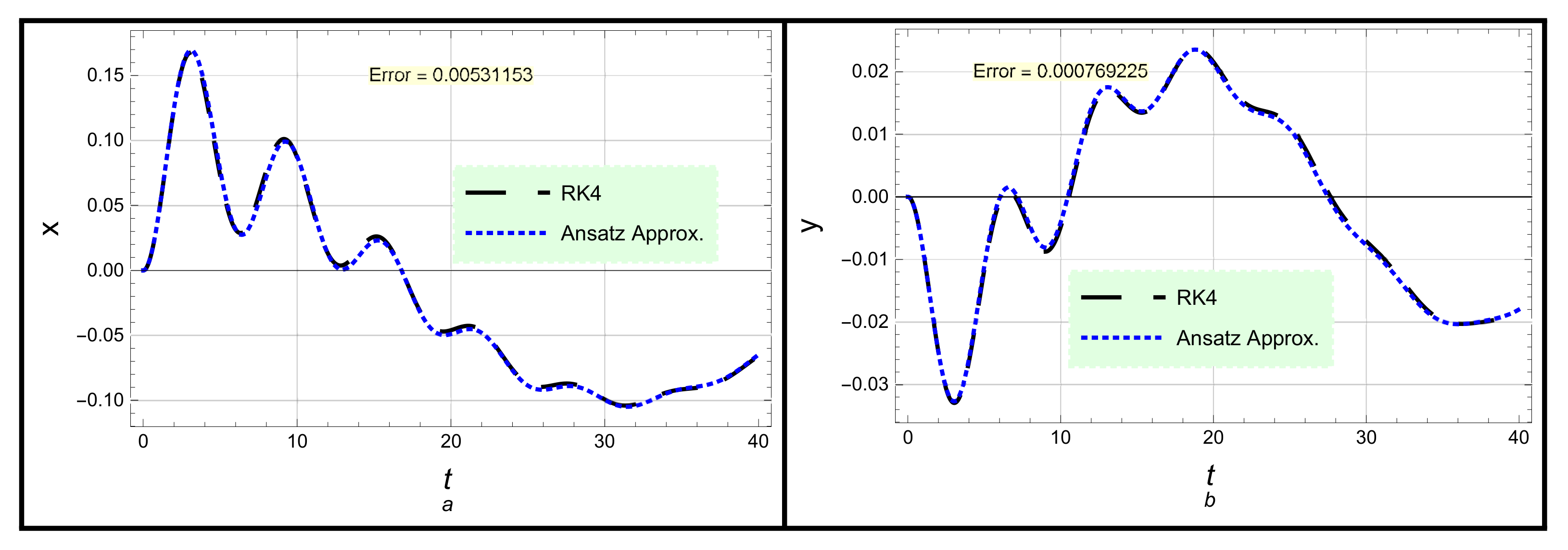
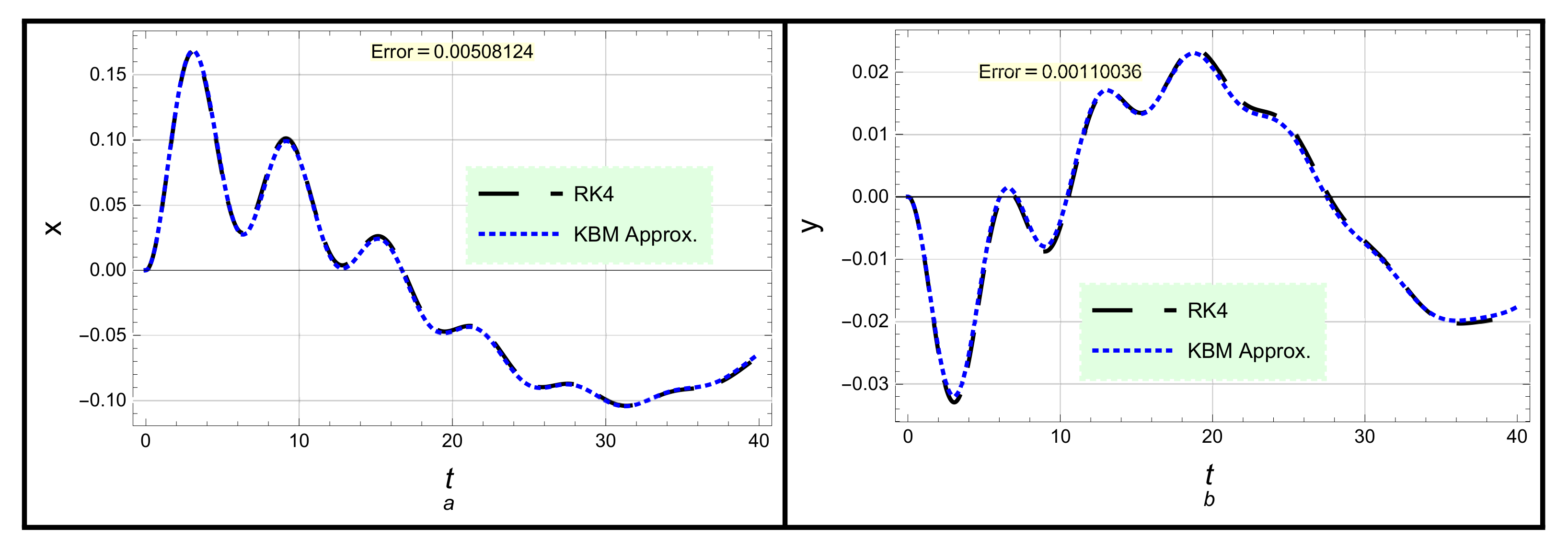
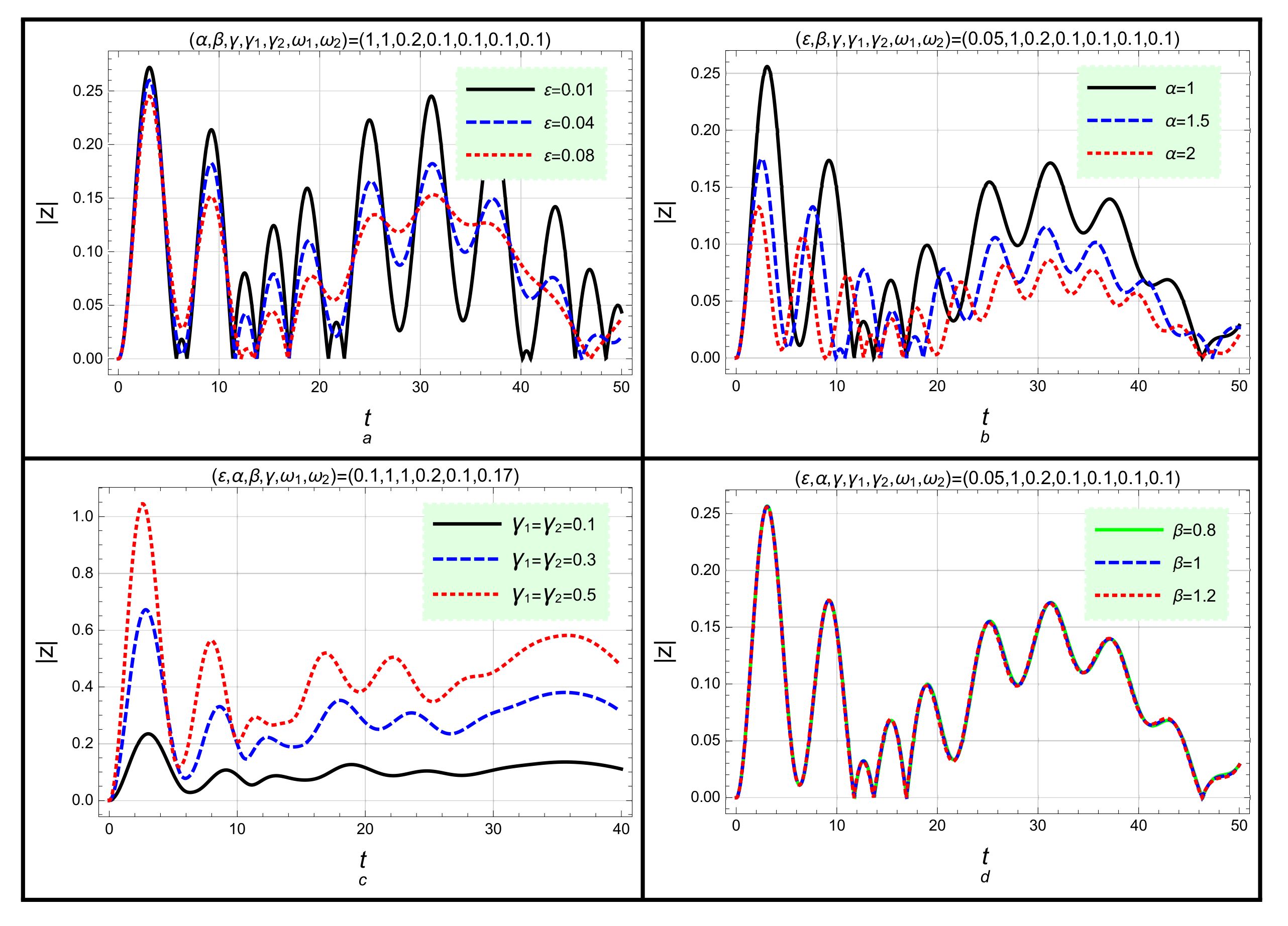
6. Results and Discussion

Let us consider the following numerical example for the first model of the FDCDO (I):

$$\left\{\begin{array}{c}\ddot{z}+0.2\dot{z}+z+z{\left|z\right|}^2+0.2{\overline{z}}^3=ϝ\left(t\right),\\ z\left(0\right)=0\& \dot{z}\left(0\right)=0,\end{array}\right.$$

(51)

with $f_1\left(t\right)={\gamma }_{1}cos\left({\omega }_{1}t\right)=0.1cos\left(0.1t\right)$, $f_2\left(t\right)={\gamma }_{2}cos\left({\omega }_{2}t\right)=-0.02cos\left(0.17t\right)$ and $T=40$.

Now, the ansatz approximation (29) and the KBM approximation (45) can be carried out to model the i.v.p. (51). The approximation of the real component $x\left(=u+v\right)$ and the approximation of the imaginary component $y\left(=u-v\right)$ using the ansatz approximation (29) and the KBM approximation (45) are compared with the numerical approximations using the RK4 approach, as illustrated in Figure 1 and Figure 2. In addition, the numerical approximations for both the real and imaginary components $\left(x,y\right)$ using the FDM are compared with the numerical RK4 approximations, as depicted in Figure 3. In addition, the absolute analytical approximations of $\left|z\right|$ using approximations (29) and (45) are compared with the absolute numerical RK4 approximations, as illustrated in Figure 4. Moreover, the numerical approximation using the FDM for the absolute $\left|z\right|$ is compared with the numerical RK4 approximation, as seen in Figure 5. Furthermore, the MRDE $L_{MRDE}$ for all obtained approximations in comparison with that of the numerical RK4 approximation is estimated, as shown in

Table 1. The estimation of the MRDE $L_{MRDE}$ for all obtained approximations.

Approximation	${\left.{\mathit{L}}_{\mathbf{MRDE}}\right|}_{\mathit{x}}$	${\left.{\mathit{L}}_{\mathbf{MRDE}}\right|}_{\mathit{y}}$	${\left.{\mathit{L}}_{\mathbf{MRDE}}\right|}_{\left|\mathit{z}\right|}$
Ansatz Approx.	$0.00531153$	$0.000769225$	$0.00534933$
KBM Approx.	$0.00508124$	$0.00110036$	$0.00511926$
FDM Approx.	$0.00157888$	$0.000318576$	$0.0016104$

. Remember that the following formulas are used to estimate the MRDE $L_{MRDE}$: ${\left.L_{MRDE}\right|}_x=\left|x-Re\left(\mathrm{RK}4\right)\right|$, ${\left.L_{MRDE}\right|}_y=\left|y-Im\left(\mathrm{RK}4\right)\right|$, and ${\left.L_{MRDE}\right|}_{\left|z\right|}=\left|\left|z\right|-\left|\mathrm{RK}4\right|\right|$.

The tabulated and graphical findings show that all of the analytical and numerical approximations have a high degree of accuracy and are more stable with respect to long periods of time. However, the analytical KBM approximations are more accurate than the ansatz approximations, but they are less accurate than the numerical FDM approximations. In the same way, all obtained analytical and numerical approximations can be applied in order to model the second model of the FDCDO (II) (13) and many other models.

The impacts of some related parameters on the profile of the FDCDO (I) (3) are investigated in Figure 6. It is observed that the amplitude of the oscillator decreases with the enhancement of $\left(\epsilon ,\alpha \right)$, while increasing both $\left({\gamma }_1,{\gamma }_2\right)$ would lead to an increase in the oscillator amplitude. The amplitude is somewhat insensitive to other parameters, such as $\left(\beta ,\gamma \right)$. For some physical applications, such as plasma physics, the fluid equations for some plasma models can be reduced to a nonlinear Schrödinger-type equation by using a reductive perturbation method [20]. Subsequently, the nonlinear Schrödinger-type equation [20,21] can be reduced to a CDO by using a suitable transformation. After that, the obtained approximations can be implemented to study the impacts of the plasma parameters on the profile of the CDO.

7. Conclusions

Nonlinear complex Duffing oscillators, including a damped complex Duffing oscillator (CDO) and a forced and damped CDO, were analyzed and solved by using some different analytical and numerical approaches. Two different general models of the forced and damped CDO, which are known as the forced and damped CDO (I) and the forced and damped CDO (II), were analyzed and discussed via both the ansatz method and the KBM approach. Accordingly, some accurate analytic approximations were derived in the terms of trigonometric functions for both the unforced and damped CDO and the forced and damped CDO. All analytical approximations that were obtained were compared with the numerical approximations when using both the fourth-order Runge–Kutta (RK4) method and the finite difference method (FDM). The distinguishing feature of the numerical methods is that of obtaining numerical approximations without decoupling in the original coupled models. To verify the accuracy of the obtained approximations, the maximum residual distance error was estimated in the whole study domain, as compared with that in the numerical RK4 approximations. It was found that the obtained approximations exhibited good accuracy and prolonged stability. However, it was noticed that the second analytic approximation (45) was a little more accurate than the first one (29).

References

1. Cveticanin, L. Analytic solution of the system of two coupled differential equations with the fifth-order non-linearity. Physica A 2003, 317, 83–94. [Google Scholar] [CrossRef]
2. Cveticanin, L. Analytic approach for the solution of the complex-valued strong non-linear differential equation of Duffing type. Physica A 2001, 297, 348–360. [Google Scholar] [CrossRef]
3. Nayfeh, A.H.; Zavodney, L.D. Experimental observation of amplitude and phase modulated responses of two internally coupled oscillators to a harmonic excitation. J. Appl. Mech. 1988, 55, 706–710. [Google Scholar] [CrossRef]
4. Grattarola, M.; Torre, V. Necessary and suffcient conditions for synchronization of non-linear oscillator with a given class of coupling. IEEE Trans. Circuits Syst. 1977, 24, 209–215. [Google Scholar] [CrossRef]
5. Cveticanin, L. Approximate analytical solutions to a class of nonlinear equations with complex functions. J. Sound Vib. 1992, 157, 289–302. [Google Scholar] [CrossRef]
6. Mahmoud, G.M. Approximate solutions of a class of complex nonlinear dynamical systems. Physica A 1998, 253, 211–222. [Google Scholar] [CrossRef]
7. Manasevich, R.; Mawhin, J.; Zanolin, F. Periodic solutions of some complex-valued Lienard and Rayleigh equations. Nonlinear Anal. 1999, 36, 997–1014. [Google Scholar] [CrossRef]
8. Cveticanin, L. An approximate solution for a system of two coupled differential equations. J. Sound Vib. 1992, 152, 375–380. [Google Scholar] [CrossRef]
9. Alhejaili, W.; Salas, A.H.; El-Tantawy, S.A. Approximate solution to a generalized Van der Pol equation arising in plasma oscillations. AIP Adv. 2022, 12, 105104. [Google Scholar] [CrossRef]
10. El-Tantawy, S.A.; Alharthi, M.R. Novel solutions to the (un)damped Helmholtz-Duffing oscillator and its application to plasma physics: Moving boundary method. Phys. Scr. 2021, 96, 104003. [Google Scholar]
11. Anh, N.D.; Hai, N.Q.; Hieu, D.V. The equivalent linearization method with a weighted averaging for analyzing of nonlinear vibrating systems. Lat. Am. J. Solids Struct. 2017, 14, 1723. [Google Scholar] [CrossRef]
12. Hieu, D.V.; Hai, N.Q.; Hung, D.T. The Equivalent Linearization Method with a Weighted Averaging for Solving Undamped Nonlinear Oscillators. J. Appl. Math. 2018, 2018, 7487851. [Google Scholar] [CrossRef] [Green Version]
13. Hieu, D.V. A New Approximate Solution for a Generalized Nonlinear Oscillator. Int. J. Appl. Comput. Math. 2019, 5, 126. [Google Scholar] [CrossRef]
14. Kadji, H.E.; Orou, J.C.; Woafo, P. Regular and chaotic behaviors of plasma oscillations modeled by a modified Duffing equation. Phys. Scr. 2008, 77, 025503. [Google Scholar] [CrossRef]
15. Salas, A.H.; Hammad, M.A.; Alotaibi, B.M.; El-Sherif, L.S.; El-Tantawy, S.A. Analytical and Numerical Approximations to Some Coupled Forced Damped Duffing Oscillators. Symmetry 2022, 14, 2286. [Google Scholar] [CrossRef]
16. He, J.H. Some asymptotic methods for strongly nonlinear equations. Int. J. Mod. Phys. B 2006, 20, 1141–1199. [Google Scholar] [CrossRef] [Green Version]
17. He, J.H. An improved amplitude-frequency formulation for nonlinear oscillators. Int. J. Nonlinear Sci. Numer. Simul. 2008, 9, 211–212. [Google Scholar] [CrossRef]
18. El-Tantawy, S.A.; Salas Alvaro, H.; Alharthi, M.R. A new approach for modelling the damped Helmholtz oscillator: Applications to plasma physics and electronic circuits. Commun. Theor. Phys. 2021, 73, 035501. [Google Scholar] [CrossRef]
19. Alhejaili, W.; Salas, A.H.; El-Tantawy, S.A. Novel Approximations to the (Un)forced Pendulum–Cart System: Ansatz and KBM Methods. Mathematics 2022, 10, 2908. [Google Scholar] [CrossRef]
20. El-Tantawy, S.A.; Salas, A.H.; Alharthi, M.R. On the Analytical and Numerical Solutions of the Linear Damped NLSE for Modeling Dissipative Freak Waves and Breathers in Nonlinear and Dispersive Mediums: An Application to a Pair-Ion Plasma. Front. Phys. 2021, 9, 580224. [Google Scholar] [CrossRef]
21. Cao, Q.H.; Dai, C.Q. Symmetric and Anti-Symmetric Solitons of the Fractional Second- and Third-Order Nonlinear Schrödinger Equation. Chin. Phys. Lett. 2021, 38, 090501. [Google Scholar] [CrossRef]
Figure 1. Both the analytic approximation (29) using the ansatz method and the RK4 approximation to the i.v.p. (6) for (a) the real and (b) imaginary components x , y are considered.
Mathematics 10 04475 g001
Figure 2. Both the analytic approximation (45) using the KBM method and the RK4 approximation to the i.v.p. (6) for (a) the real and (b) imaginary components x , y are considered.
Mathematics 10 04475 g002
Figure 3. The numerical approximations for (a) the real and (b) imaginary components x , y using the FDM are compared with the RK4 numerical approximations.
Mathematics 10 04475 g003
Figure 4. (a) The analytic approximation (29) using the ansatz method and (b) the analytic approximation (45) using the KBM method for the absolute value of | z | are compared with the numerical RK4 approximations of the i.v.p. (6).
Mathematics 10 04475 g004
Figure 5. The numerical approximation for the absolute value | z | using the FDM is compared with the numerical RK4 approximation.
Mathematics 10 04475 g005
Figure 6. The impacts of the coefficients (a) ε , (b) α , (c) γ 1 , γ 2 , and (d) β on the profile of the forced and damped CDO (I) (3) according to the analytic approximation (29).
Mathematics 10 04475 g006