
Radii of Starlikeness of Ratios of Analytic Functions with Fixed Second Coefficients


Abstract
1. Introduction
2. Analysis and Mapping of for , and
3. Radius of Starlikeness
- 1.
- For the class , the sharp radius is the smallest root of the equation , where.
- 2.
- For the class , the sharp radius is the smallest root of the equation , where
- 3.
- For the class , the sharp radius is the smallest root of the equation , where.
- Note that and ; thus, in view of the Intermediate Value Theorem, there exists a root of the equation in the interval . Let be the smallest root of the equation . For , using (5), we havewhich yieldswhenever . This shows that for .This proves that the radius is sharp.
- A calculation shows that and . By the Intermediate Value Theorem, there exists a root of the equation . Let be the smallest root of the equation and . An easy calculation shows that, for ,where and are given by (1). From (9) and (11) and using Lemma 2 together with (23), we havewhenever . Thus, for . To prove the sharpness, consider the function defined byandwhere and Note that, for ,andwhereare Schwarz functions; hence, , , and . For , and , it follows from (24) that
- It is easy to see that and . By the Intermediate Value Theorem, there exists a root of the equation . Let be the smallest root of the equation . From (18), it follows that, for any ,whenever . This proves that for . The result is sharp for the function defined for the class in (20). At and for , it follows from (25) that
- 1.
- For the class , the sharp radius is the smallest root of the equation , where
- 2.
- For the class , the sharp radius is the smallest root of the equation , where
- 3.
- For the class , the sharp radius is the smallest root of the equation , where.
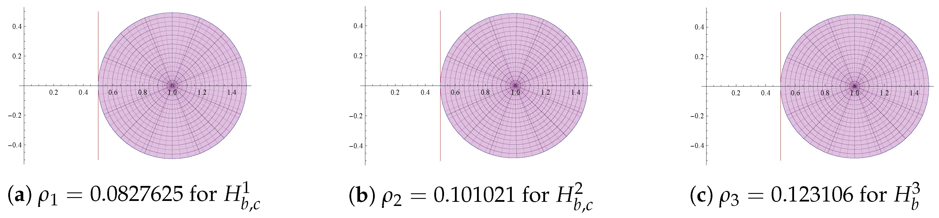
- 1.
- For the class , the sharp radius is the smallest root of the equation , where.
- 2.
- For the class , the sharp radius is the smallest root of the equation , where.
- 3.
- For the class , the sharp radius is the smallest root of the equation , where.
- Note that and ; thus, in view of the Intermediate Value Theorem, there exists a root of the equation in the interval . Let be the smallest root of the equation . Ali et al. [30] (Lemma 2.2) proved that, forIn view of (26) and the fact that the centre of the disc in (21) is 1, ifwhich is equivalent to if . Since and is the smallest root of the equation , is an increasing function on . In view of this for . For , , using (27), the function defined for the class in (6) at satisfies the following equalityThus, the radius is sharp.
- A calculation shows that and . By the Intermediate Value Theorem, there exists a root of the equation . Let be the smallest root of the equation , and . As the centre of the disc in (13) is 1, by (26), ifwhich is equivalent to if . Since and is the smallest root of the equation , is an increasing function on . Thus, for . To prove the sharpness, consider the function defined in (14). For , and , it follows from (28) that
- It is easy to see that and . By the Intermediate Value Theorem, there exists a root of the equation . Let be the smallest root of the equation . From (16) and (17) it follows that, for any
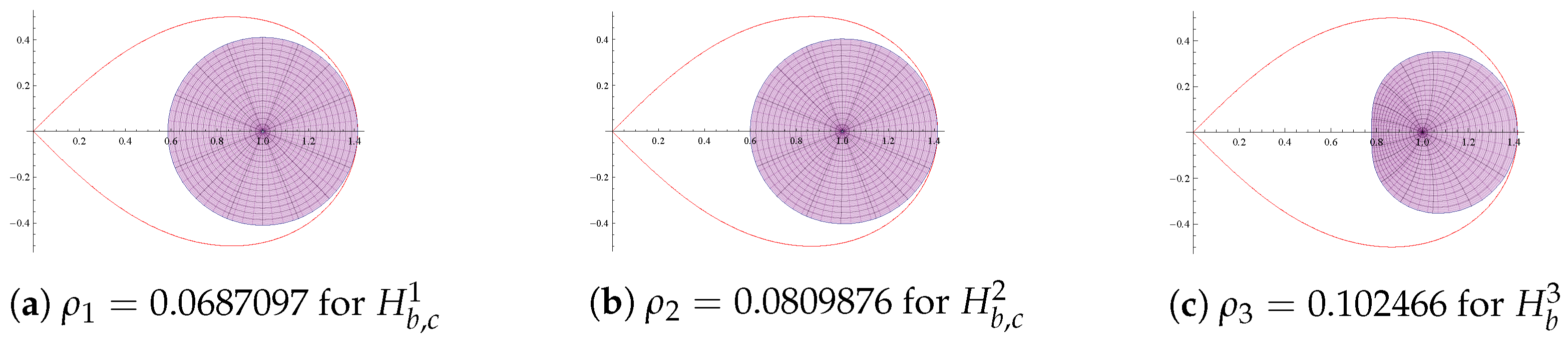
- 1.
- For the class , the sharp radius is the smallest root of the equation , where
- 2.
- For the class , radius is the smallest root of the equation , where
- 3.
- For the class , the sharp radius is the smallest root of the equation , where
- Note that and ; thus, in view of the Intermediate Value Theorem, there exists a root of the equation in the interval . Let be the smallest root of the equation . Shanmughan and Ravichandran (p. 321, [34]) proved, for thatAs the centre of the disc in (21) is 1, by (31), ifwhich is equivalent to if . Since and is the smallest root of the equation , is an increasing function on . In view of this, for . For , , using (32), the function defined for the class in (8) at , satisfies the following equalityThis proves that the radius is sharp.
- A calculation shows that and, which is greater than 0. By the Intermediate Value Theorem, there exists a root of the equation . Let be the smallest root of the equation and . From (9) and (11) and using Lemma 2 together with (23), we havewhenever . Since and is the smallest root of the equation , is an increasing function on . Thus, for .
- It is easy to see that and . By the Intermediate Value Theorem, there exists a root of the equation . Let be the smallest root of the equation . In view of (31) and the fact that the centre of the disc in (29) is 1, ifwhich is equivalent to if . Since and is the smallest root of the equation , is an increasing function on . This proves that for .
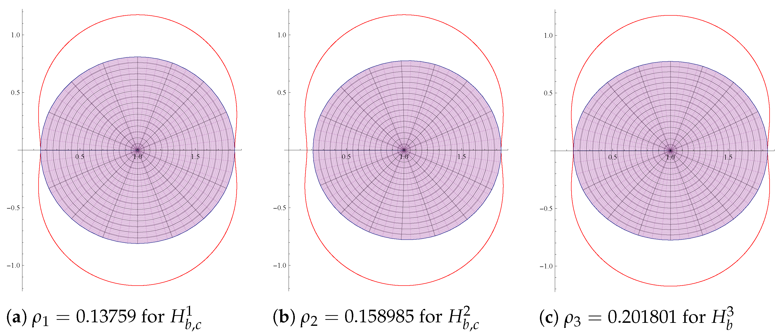
- 1.
- For the class , the sharp radius is the smallest root of the equation , where.
- 2.
- For the class , radius is the smallest root of the equation , where
- 3.
- For the class , the sharp radius is the smallest root of the equation , where.
- Note that and ; thus, in view of the Intermediate Value Theorem, there exists a root of the equation in the interval . Let be the smallest root of the equation . Mendiratta et al. [35] proved, for , thatAs the centre of the disc in (21) is 1, by (34), ifwhich is equivalent to if . Since and is the smallest root of the equation , is an increasing function on . In view of this, for . For , , using (35), the function defined for the class in (8) at , satisfies the following equality,Thus, the radius is sharp.
- A calculation shows that and . By the Intermediate Value Theorem, there exists a root of the equation . Let be the smallest root of the equation and . In view of (34) and the fact that the centre of the disc in (13) is 1, ifwhich is equivalent to if . Since and is the smallest root of the equation , is an increasing function on . Thus, for .
- It is easy to see that and . By the Intermediate Value Theorem, there exists a root of the equation . Let be the smallest root of the equation . Since the centre of the disc in (29) is 1, by (34), ifwhich is equivalent to if . Since and is the smallest root of the equation , is an increasing function on . This proves that for .
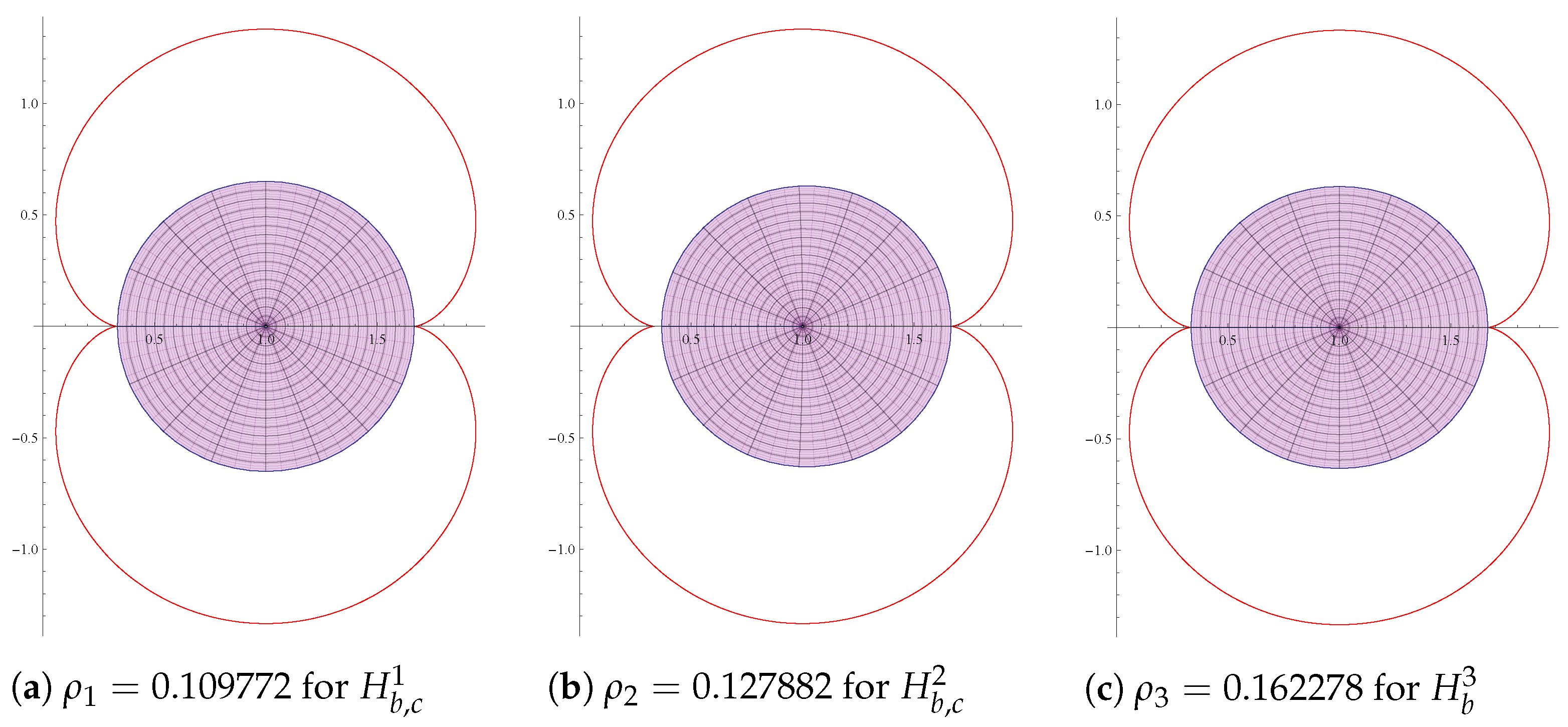
- 1.
- For the class , the sharp radius is the smallest root of the equation , where.
- 2.
- For the class , the radius is the smallest root of the equation , where.
- 3.
- For the class , the sharp radius is the smallest root of the equation , where.
- Note that and ; thus, in view of the Intermediate Value Theorem, there exists a root of the equation in the interval . Let be the smallest root of the equation . Sharma et al. [36] proved that, for ,As the centre of the disc in (21) is 1, by (37), ifwhich is equivalent to if . Since and is the smallest root of the equation , is an increasing function on . In view of this for . For , , using (38), the function defined for the class in (8) at , satisfies the following equalitywhich belongs to boundary of the region . Thus, the radius is sharp.
- A calculation shows that and . By the Intermediate Value Theorem, there exists a root of the equation . Let be the smallest root of the equation and . In view of (37) and the fact that the centre of the disc in (13) is 1, ifwhich is equivalent to if . Since and is the smallest root of the equation , is an increasing function on . Thus, for .
- It is easy to see that and . By the Intermediate Value Theorem, there exists a root of the equation . Let be the smallest root of the equation . In view of the fact that the centre of the disc in (29) is 1, by (37), ifwhich is equivalent to if . Since and is the smallest root of the equation , is an increasing function on . This proves that for .
- 1.
- For the class , the sharp radius is the smallest root of the equation , where.
- 2.
- For the class , the sharp radius is the smallest root of the equation , where.
- 3.
- For the class , the sharp radius is the smallest root of the equation , where.
- Note that and ; thus, in view of the Intermediate Value Theorem, there exists a root of the equation in the interval . Let be the smallest root of the equation . For Cho et al. [37] established the following inclusion property,where is the image of the unit disc under the mappings . As the centre of the disc in (21) is 1, by (40), ifwhich is equivalent to if . Since and is the smallest root of the equation , is an increasing function on . In view of this for . For , , using (41), the function defined for class in (6) at , satisfies the following equalitywhich belongs to the boundary of region . This proves the radius is sharp.
- A calculation shows that and . By the Intermediate Value Theorem, there exists a root of the equation . Let be the smallest root of equation and . In view of (40) and the fact that centre of the disc in (13) is 1, ifwhich is equivalent to if . Since and is the smallest root of the equation , is an increasing function on . Thus, for . To prove sharpness, consider the function defined in (14). For , and , it follows from (42) thatwhich illustrates the sharpness.
- It is easy to see that and . By the Intermediate Value Theorem, there exists a root of the equation . Let be the smallest root of the equation . Since the centre of the disc in (29) is 1, by (40), ifwhich is equivalent to if . Since and is the smallest root of the equation , is an increasing function on This proves that for .
- 1.
- For the class , the sharp radius is the smallest root of the equation , where.
- 2.
- For the class , the radius is the smallest root of the equation , where.
- 3.
- For the class , the sharp radius is the smallest root of the equation , where.
- Note that and ; thus, in view of the Intermediate Value Theorem, there exists a root of the equation in the interval . Let be the smallest root of the equation . Gandhi and Ravichandran [39] (Lemma 2.1) proved that, for ,As the centre of the disc in (21) is 1, by (44), ifwhich is equivalent to if . Since and is the smallest root of the equation , is an increasing function on . In view of this for . For , , using (45), the function defined for the class in (8) at , satisfies the following equalityThis proves the sharpness.
- A calculation shows that and . By the Intermediate Value Theorem, there exists a root of the equation . Let be the smallest root of the equation and . In view of (44) and the fact centre of the disc in (13) is 1, ifwhich is equivalent to if . Since and is the smallest root of the equation , is an increasing function on . Thus, for .
- It is easy to see that and . By the Intermediate Value Theorem, there exists a root of the equation . Let be the smallest root of the equation . Since the centre of the disc in (29) is 1, by (44), ifwhich is equivalent to if . Since and is the smallest root of the equation , is an increasing function on This proves that for .
- 1.
- For the class , the sharp radius is the smallest root of the equation , where.
- 2.
- For the class , the radius is the smallest root of the equation , where.
- 3.
- For the class , the sharp radius is the smallest root of the equation , where
- Note that and ; thus, in view of the Intermediate Value Theorem, there exists a root of the equation in the interval . Let be the smallest root of the equation . For Kumar et al. [40] proved thatAs the centre of the disc in (21) is 1, by (47) ifwhich is equivalent to if . Since and is the smallest root of the equation , is an increasing function on . In view of this for . For , , using (48), the function defined for the class in (8) at , satisfies the following equalityThis proves the sharpness.
- A calculation shows that and . By the Intermediate Value Theorem, there exists a root of the equation . Let be the smallest root of the equation and . In view of (47) and the fact that the centre of the disc in (13) is 1, ifwhich is equivalent to if . Since and is the smallest root of the equation , is an increasing function on . Thus, for .
- It is easy to see that and . By the Intermediate Value Theorem, there exists a root of the equation . Let be the smallest root of the equation . Since the centre of the disc in (29) is 1, by (47), ifwhich is equivalent to if . Since and is the smallest root of the equation , is an increasing function on This proves that for .
- 1.
- For the class , the sharp radius is the smallest root of the equation , where.
- 2.
- For the class , the sharp radius is the smallest root of the equation , where
- 3.
- For the class , the sharp radius is the smallest root of the equation , where.
- Note that and ; thus, in view of the Intermediate Value Theorem, there exists a root of the equation in the interval . Let be the smallest root of the equation . For Wani and Swaminathan [41] (Lemma 2.2) had proved thatAs the centre of the disc in (21) is 1, by (50), ifwhich is equivalent to if . Since and is the smallest root of the equation , is an increasing function on . In view of this for . For , , using (51), the function defined for the class in (6) at , satisfies the following equalitywhich belongs to the boundary of the region . This proves sharpness.
- A calculation shows that and . By the Intermediate Value Theorem, there exists a root of the equation . Let be the smallest root of the equation and . In view of (50) and the fact that centre of the disc in (13) is 1, ifwhich is equivalent to if . Since and is the smallest root of the equation , is an increasing function on . Thus, for . To prove the sharpness, consider the function defined in (14). For , and , it follows from (52) thatwhich illustrates the sharpness.
- It is easy to see that and . By the Intermediate Value Theorem, there exists a root of the equation . Let be the smallest root of the equation . Since the centre of the disc in (29) is 1, by (50), ifwhich is equivalent to if . Since and is the smallest root of the equation , is an increasing function on This proves that for .
- 1.
- For the class , the sharp radius is the smallest root of the equation , where
- 2.
- For the class , the sharp radius is the smallest root of the equation , where
- 3.
- For the class , the sharp radius is the smallest root of the equation , where
- Note that and . In view of the Intermediate Value Theorem, there exists a root of the equation in the interval . Let be the smallest root of the equation . For Goel and Kumar [42] proved the following inclusion property,As the centre of the disc in (21) is 1, by (54), ifwhich is equivalent to if . Since and is the smallest root of the equation , is an increasing function on . In view of this for . For , , using (55), the function defined for the class in (6) at , satisfies the following equalityIt follows that the radius is sharp.
- A calculation shows that and . By the Intermediate Value Theorem, there exists a root of the equation . Let be the smallest root of the equation and . In view of (54) and the fact that the centre of the disc in (13) is 1, ifwhich is equivalent to if . Since and is the smallest root of the equation , is an increasing function on . Thus, for . To prove the sharpness, consider the function defined in (14). For , and , the similar calculations as in (56) together with (57) proves that the result is sharp.
- It is easy to see that and . By the Intermediate Value Theorem, there exists a root of the equation . Let be the smallest root of the equation . Since the centre of the disc in (29) is 1, by (54), ifwhich is equivalent to if . Since and is the smallest root of the equation , is an increasing function on This proves that for .At and for , a calculation as in part(i) shows that the result is sharp for the function defined for the class in (20)
4. Conclusions
Author Contributions
Funding
Institutional Review Board Statement
Informed Consent Statement
Data Availability Statement
Acknowledgments
Conflicts of Interest
References
- Gronwall, T.H. On the distortion in conformal mapping when the second coefficient in the mapping function has an assigned value. Nat. Acad. Proc. 1920, 6, 300–302. [Google Scholar] [CrossRef] [PubMed]
- Ali, R.M.; Nagpal, S.; Ravichandran, V. Second-order differential subordination for analytic functions with fixed initial coefficient. Bull. Malays. Math. Sci. Soc. (2) 2011, 34, 611–629. [Google Scholar]
- Lee, S.K.; Ravichandran, V.; Supramaniam, S. Applications of differential subordination for functions with fixed second coefficient to geometric function theory. Tamsui Oxf. J. Inf. Math. Sci. 2013, 29, 267–284. [Google Scholar]
- Kumar, S.; Ravichandran, V.; Verma, S. Initial coefficients of starlike functions with real coefficients. Bull. Iranian Math. Soc. 2017, 43, 1837–1854. [Google Scholar]
- Ahuja, O.P. The influence of second coefficient on spiral-like and the Robertson functions. Yokohama Math. J. 1986, 34, 3–13. [Google Scholar]
- Ahuja, O.P.; Silverman, H. Extreme points of families of univalent functions with fixed second coefficient. Colloq. Math. 1987, 54, 127–137. [Google Scholar] [CrossRef]
- Ali, R.M.; Kumar, V.; Ravichandran, V.; Kumar, S.S. Radius of starlikeness for analytic functions with fixed second coefficient. Kyungpook Math. J. 2017, 57, 473–492. [Google Scholar]
- Ali, R.M.; Cho, N.E.; Jain, N.K.; Ravichandran, V. Radii of starlikeness and convexity for functions with fixed second coefficient defined by subordination. Filomat 2012, 26, 553–561. [Google Scholar] [CrossRef]
- Nehari, Z. Conformal Mapping; McGraw-Hill Book Co., Inc.: New York, NY, USA, 1952. [Google Scholar]
- Ma, W.C.; Minda, D. A unified treatment of some special classes of univalent functions. In Proceedings of the Conference on Complex Analysis (Tianjin, 1992); Conf. Proc. Lecture Notes Anal., I; Int. Press: Cambridge, MA, USA, 1992; pp. 157–169. [Google Scholar]
- Ma, W.C.; Minda, D. Uniformly convex functions. Ann. Polon. Math. 1992, 57, 165–175. [Google Scholar] [CrossRef]
- MacGregor, T.H. The radius of convexity for starlike functions of order 12. Proc. Amer. Math. Soc. 1963, 14, 71–76. [Google Scholar]
- Anand, S.; Jain, N.K.; Kumar, S. Normalized analytic functions with fixed second coefficient. J. Anal. to appear.
- Lecko, A.; Ravichandran, V.; Sebastian, A. Starlikeness of certain non-univalent functions. Anal. Math. Phys. 2021, 11, 163. [Google Scholar] [CrossRef]
- MacGregor, T.H. The radius of univalence of certain analytic functions. Proc. Amer. Math. Soc. 1963, 14, 514–520. [Google Scholar] [CrossRef]
- MacGregor, T.H. The radius of univalence of certain analytic functions. II. Proc. Amer. Math. Soc. 1963, 14, 521–524. [Google Scholar] [CrossRef]
- Ratti, J.S. The radius of convexity of certain analytic functions. Indian J. Pure Appl. Math. 1970, 1, 30–36. [Google Scholar] [CrossRef]
- Ratti, J.S. The radius of univalence of certain analytic functions. Math. Z. 1968, 107, 241–248. [Google Scholar] [CrossRef]
- El-Faqeer, A.S.A.; Mohd, M.H.; Ravichandran, V.; Supramaniam, S. Starlikeness of certain analytic functions. Appl. Math. -Notes 2022, 22, 516–528. [Google Scholar]
- Kanaga, R.; Ravichandran, V. Starlikeness for certain close-to-star functions. Hacet. J. Math. Stat. 2021, 50, 414–432. [Google Scholar] [CrossRef]
- Lee, S.K.; Khatter, K.; Ravichandran, V. Radius of starlikeness for classes of analytic functions. Bull. Malays. Math. Sci. Soc. 2020, 43, 4469–4493. [Google Scholar] [CrossRef]
- Sebastian, A.; Ravichandran, V. Radius of starlikeness of certain analytic functions. Math. Slovaca 2021, 71, 83–104. [Google Scholar] [CrossRef]
- Ali, R.M.; Jain, N.K.; Ravichandran, V. On the radius constants for classes of analytic functions. Bull. Malays. Math. Sci. Soc. 2013, 36, 23–38. [Google Scholar]
- McCarty, C.P. Functions with real part greater than α. Proc. Amer. Math. Soc. 1972, 35, 211–216. [Google Scholar] [CrossRef]
- McCarty, C.P. Two radius of convexity problems. Proc. Amer. Math. Soc. 1974, 42, 153–160. [Google Scholar] [CrossRef]
- Hayami, T.; Owa, S. Hankel determinant for p-valently starlike and convex functions of order α. Gen. Math. 2009, 17, 29–44. [Google Scholar]
- Anand, S.; Jain, N.K.; Kumar, S. Certain estimates of normalized analytic functions. Math. Slovaca 2022, 72, 85–102. [Google Scholar] [CrossRef]
- Madaan, V.; Kumar, A.; Ravichandran, V. Starlikeness associated with lemniscate of Bernoulli. Filomat 2019, 33, 1937–1955. [Google Scholar] [CrossRef]
- Sokół, J.; Stankiewicz, J. Radius of convexity of some subclasses of strongly starlike functions. Zeszyty Nauk. Politech. Rzeszowskiej Mat. 1996, 19, 101–105. [Google Scholar]
- Ali, R.M.; Jain, N.K.; Ravichandran, V. Radii of starlikeness associated with the lemniscate of Bernoulli and the left-half plane. Appl. Math. Comput. 2012, 218, 6557–6565. [Google Scholar] [CrossRef]
- Ali, R.M.; Ravichandran, V. Uniformly convex and uniformly starlike functions. Ramanujan Math. Newsl. 2011, 21, 16–30. [Google Scholar]
- Gangadharan, A.; Ravichandran, V.; Shanmugam, T.N. Radii of convexity and strong starlikeness for some classes of analytic functions. J. Math. Anal. Appl. 1997, 211, 301–313. [Google Scholar] [CrossRef]
- Ravichandran, V.; Rønning, F.; Shanmugam, T.N. Radius of convexity and radius of starlikeness for some classes of analytic functions. Complex Variables Theory Appl. 1997, 33, 265–280. [Google Scholar] [CrossRef]
- Shanmugam, T.N.; Ravichandran, V. Certain properties of uniformly convex functions. In Computational Methods and Function Theory 1994 (Penang); Ser. Approx. Decompos., 5; World Scientific Publishing: River Edge, NJ, USA, 1995; pp. 319–324. [Google Scholar]
- Mendiratta, R.; Nagpal, S.; Ravichandran, V. On a subclass of strongly starlike functions associated with exponential function. Bull. Malays. Math. Sci. Soc. 2015, 38, 365–386. [Google Scholar] [CrossRef]
- Sharma, K.; Jain, N.K.; Ravichandran, V. Starlike functions associated with a cardioid. Afr. Mat. 2016, 27, 923–939. [Google Scholar] [CrossRef]
- Cho, N.E.; Kumar, V.; Kumar, S.S.; Ravichandran, V. Radius problems for starlike functions associated with the sine function. Bull. Iranian Math. Soc. 2019, 45, 213–232. [Google Scholar] [CrossRef]
- Raina, R.K.; Sokół, J. Some properties related to a certain class of starlike functions. C. R. Math. Acad. Sci. Paris 2015, 353, 973–978. [Google Scholar] [CrossRef]
- Gandhi, S.; Ravichandran, V. Starlike functions associated with a lune. Asian-Eur. J. Math. 2017, 10, 1750064. [Google Scholar] [CrossRef]
- Kumar, S.; Ravichandran, V. A subclass of starlike functions associated with a rational function. Southeast Asian Bull. Math. 2016, 40, 199–212. [Google Scholar]
- Wani, L.A.; Swaminathan, A. Starlike and convex functions associated with a nephroid domain. Bull. Malays. Math. Sci. Soc. 2021, 44, 79–104. [Google Scholar] [CrossRef]
- Goel, P.; Sivaprasad Kumar, S. Certain class of starlike functions associated with modified sigmoid function. Bull. Malays. Math. Sci. Soc. 2020, 43, 957–991. [Google Scholar] [CrossRef]
- Sharma, M.; Kumar, S.; Jain, N.K. Differential subordinations for functions with positive real part using admissibility conditions. Asian-Eur. J. Math. 2022, 15, 2250066. [Google Scholar] [CrossRef]


Publisher’s Note: MDPI stays neutral with regard to jurisdictional claims in published maps and institutional affiliations. |
© 2022 by the authors. Licensee MDPI, Basel, Switzerland. This article is an open access article distributed under the terms and conditions of the Creative Commons Attribution (CC BY) license (https://creativecommons.org/licenses/by/4.0/).
Share and Cite
Rana, S.; Ahuja, O.P.; Jain, N.K. Radii of Starlikeness of Ratios of Analytic Functions with Fixed Second Coefficients. Mathematics 2022, 10, 4428. https://doi.org/10.3390/math10234428
Rana S, Ahuja OP, Jain NK. Radii of Starlikeness of Ratios of Analytic Functions with Fixed Second Coefficients. Mathematics. 2022; 10(23):4428. https://doi.org/10.3390/math10234428
Chicago/Turabian StyleRana, Shalini, Om P. Ahuja, and Naveen Kumar Jain. 2022. "Radii of Starlikeness of Ratios of Analytic Functions with Fixed Second Coefficients" Mathematics 10, no. 23: 4428. https://doi.org/10.3390/math10234428
APA StyleRana, S., Ahuja, O. P., & Jain, N. K. (2022). Radii of Starlikeness of Ratios of Analytic Functions with Fixed Second Coefficients. Mathematics, 10(23), 4428. https://doi.org/10.3390/math10234428