An Aggregation Rule Based on the Binomial Distribution

Abstract

Many decision-making situations require the evaluation of several voters or agents. In a situation where voters evaluate candidates, the question arises of how best to aggregate evaluations so as to compare the candidates. The aim of this work is to propose a method of aggregating the evaluations of the voters, which has outstanding properties and serve as a potential evaluative tool in many contexts. Ordered weighted averages is a family of rules appropriate for studying this problem. In this paper, I propose as a solution an ordered weighted average that satisfies compelling properties and whose weights are derived from the binomial distribution.

1. Introduction

A method of aggregating scores from various voters (also known as judges) to one or more candidates is proposed in this article. The study carries out analyses of the family of ordered weighted averages and selects the one with the best properties, with the purpose to assign a fair evaluation of a single candidate and to rank fairly the candidates when they compete. A unified procedure is proposed for these two situations. I formally describe the context under study by defining three sets.

Let $N=\{1,2,\cdots ,n\}$ be the set of judges. Throughout this article I assume $n\ge 2$. Let $C=\{c_1,c_2,\cdots ,c_m\}$ be the set of candidates. I am interested in two different situations: that in which a sole candidate is evaluated, i.e., $m=1$, and that in which several candidates are evaluated and afterwards ranked, i.e., $m\ge 2$. Let $\Gamma$ be the evaluation set, through which judges express their evaluation in $\Gamma$ to each candidate. There is no restriction on the ballots or choices. For instance, a judge can assign the same evaluation to several candidates. In this article, I mainly refer to numerical evaluations that in most cases can be thought of as grades. The terms grades or scores is used interchangeably from now on. I deal with several types of sets for $\Gamma$. The most standard type for it is a finite set $\Gamma =\{g_1,\cdots ,g_{\gamma }\}$ of cardinality $\gamma \ge 2$. The evaluations are numerical (Grades can also be qualitative, (e.g., $\Gamma =\{1,2,3,4,5\}$ can be also thought of as $\Gamma =\{A,B,C,D,E\}$) if there is a bijection between the two sets, i.e., if they can be thought of as equivalent forms of grading.) (e.g., $\Gamma =\{0,1,2,\cdots ,9,10\}$ or $\Gamma =\{1,2,3,4,5\}$), being equally spaced, i.e., $g_{i+1}-g_i=ϵ>0$ for all $i=1,\cdots ,\gamma -1$. However, practically everything exposed in the article also applies to larger sets where grades’ equidistance is not required, or more generally, continuous intervals of real numbers, such as, for example, $\Gamma =[0,1]$, (The continuous set $[0,1]$ can also be understood as a normalization of any other closed, bounded and convex set.) so that the judges can express their evaluation from a finer grid.

The case of several candidates has been extensively studied. In fact, additive rules, close solutions to the mean, interpret the evaluations as grades selecting as winner the candidate with the highest total grade. They are sometimes referred to as “utilitarian” voting rules, [1]. Two characterization results for additive rules are provided in [2]: evaluative voting and range voting. Other rules are conceivable as well, such as comparing candidates according to their median evaluation, see [3], or to their minimum evaluation [4]. The rule I propose in this paper is an alternative to all these proposals.

This work on voting rules is connected to game theory in the following sense. A voting method is identified with a game structure. The voters are the players, the social decisions to be adopted are the alternatives, the strategies are the concrete ways of casting the vote available to each voter and the aggregation function incorporates the set of rules through which is determined the social decision to adopt.

The remainder of this section provides motivating examples of real situations coming from very different backgrounds. The other sections of this article are organized as follows. The ordered weighted averages are introduced in Section 2, as a broad class of solutions to the aggregation problem posed. Some particular ordered weighted averages are introduced in Section 3, including the new rule, which is the main objective of study in this work. Two characterizations of this rule are presented in Section 4. Section 5 highlights additional compelling properties of the rule proposed in this article. The conclusion ends the paper in Section 6.

Motivating Examples

I start by discussing several examples from very different backgrounds. In the first three examples, a single candidate is evaluated. In the next examples, various candidates are evaluated and subsequently ranked.

• Evaluating final degree projects and Ph.D. thesis: The evaluation of the project consists of the presentation and defense of an innovative work. The jury of the project is usually made up of three or five professors. It is usually five when it comes to doctoral theses. Each member of the committee proposes a grade. The final qualification awarded by the committee is deduced from the individual grades. Some aspects are crucial for the student: pass or not, cum laude or not.
  The mean of the individual grades is often used to obtain the student’s final grade. For instance, assume that the grades are $5,5,9,9,10$ on an integer scale from 0 to 10. The mean is $7.5$, the median is 9 and the proposed rule in this paper yields $7.8125$.
• Judging professors by students in universities: Students evaluate their professors according to their satisfaction with their teaching performance. They are allowed to assign an integer number from one (very unsatisfactory) to five (very satisfactory). Thus, each professor gets a score between one and five per course, which is the mean of students’ scores. A professor usually teaches between 10 and 20 courses every five years, and therefore obtains an aggregated score of the five-year period, which is again the mean of all the courses taught.
  Professors can request a teaching supplement every 5 years. A very important criterion is the assessment obtained by students during these 5 years. A professor needs a minimum mark of three to obtain the five-year teaching supplement. For instance, assume the scores per course obtained by a professor in the 10 courses taught in a five-year period were:

  $$1.5,1.5,2,3,3.2,3.2,3.2,3.6,3.8,4.$$
  The mean is $2.9$ which has fatal consequences for the professor, the median is $3.2$ and the proposed rule is $3.09$.
• Rating companies by debt agencies: Debt rating agencies (such as Standard and Poors, Fitch, Moody’s or DBR, among others) evaluate companies. They use a rating scale, which goes from the best evaluation to the worst evaluation and comprises 21 degrees. The rating scale is mainly divided into two sections or categories: investment (from 1st to 10th) and speculative (from 11th to 21st). Different agencies provide company rankings simultaneously. The way their qualifications are aggregated is fundamental for the company, investors of the company and potential future investors. Assume, that the qualifications of the four agencies for a certain company are: $8,9,10,14$. If the mean, which is over 10, is used to aggregate these evaluations, the company’s category is declared speculative. Instead, the proposed rule assigns 10, which corresponds to the last level of investment category. Note that in this example, I have taken the ordinal criterion so that the lower the number, the better the rating.
• Doctoral student selection problem: Some universities offer programs for gaining the doctoral (Ph.D.) degree. The process to select students is open to students from everywhere. In most of the cases, the number of applicants is much greater than the number of available scholarships, so the candidates must be ranked. The problem of selecting young promising doctoral researchers can be seen to consist of a collection of applicants for the Ph.D. program and a set of experts who grade each applicant by using a pre-established set of allowed scores. An application of this problem at the Graduate School of Turku Center for Computer Science in Finland has been studied by using ordered weighted averages in [5].
• Artistic sports competitions: Some sports competitions require the evaluation of athletes performance by a panel of judges, such as diving, artistic skating, gymnastics, rhythmic gymnastics, dancing, riding, etc. The rules used are very diverse and range from the mean (used by several federations, for example, the International Federation for Equestrian Sports), the median (the synthesis of the scores of each subjury in rhythmic gymnastics is a median), trimmed means (used in various cases of diving) to some sophisticated methods. Other interesting techniques have been proposed by Crowley [6] or Gambarelli [7]. Both used the arithmetic mean of some scores. The first technique was based on discarding a fixed number of scores being the furthest from the median, while the second only discards scores when these were considered to be inappropriate. Regulations of some international federations collect the use of these rules, see, e.g., [8].
• Judging the judges: Federations, companies or universities are also interested in evaluating the judges that make up the evaluation panel after each evaluative activity. Judges that are too strict or not rigorous enough with the majority of the candidates are less appropriate for the constitution of new panels. Neither the mean nor the median are useful rules for detecting such extreme form of grading. The rule proposed in the article is also ideal for detecting these profiles of judges and therefore to establish rankings of judges based on their past performances as judges.

The following two examples are similar to the fourth one described above, so I omit their description here. I just point out relevant aspects of them.

7.

Ranking of research projects by scientific committees: The main distinction with the fourth example above is that in this example, the expected number of applicants is usually huge.

8.

Ranking of restaurants or movies on designed websites: At a given time, the set N is large and formed from all the people who have rated these restaurants or these movies. In most of the previous examples, N is not necessarily large.

The rule presented in Section 3 of this paper is useful for all these contexts.

2. Ordered Weighted Averages

Following [9], aggregation is the process of combining several numerical values into a single representative one, a procedure called an aggregation function. Despite the simplicity of this definition, the size of the field of its applications is incredibly huge. Making decisions (in artificial intelligence as well) often leads to aggregating preferences or scores on a given set of alternatives. The concept of the ordered weighted averaging operator was introduced by Yager, [10] and intensively developed in [11] and subsequent works. Since then, these functions have been axiomatized and extended in various ways. The development of an appropriate methodology for obtaining the weights is still an issue of great interest. This work is a contribution in the search for appropriate weights for several decision-making problems.

Formally, an ordered weighted average (OWA) operator of dimension n is a mapping $G^n:{\mathbb{R}}^n\to \mathbb{R}$ that has an associated collection of weights $w^n=(w_1^n,\dots ,w_n^n)$ lying in the unit interval and summing to one ($w_i^n\ge 0$ for all i and ${\displaystyle \sum _{i=1}^n}{w}_i^n=1$) with

$$G^n(x_1,\dots ,x_n)=\sum _{j=1}^n{w}_j^n{y}_j$$

where $y_j$ is the jth largest element in $\{x_1,\cdots ,x_n\}$. A fundamental aspect of this operator is that the reordering step, in particular an $x_i$ is not associated with a particular weight $w_i^n$ but rather a weight is associated with a particular ordered position of the $x_i$’s. By choosing different $w^n$, one can implement different aggregation operators. The OWA operator is a nonlinear operator as a result of the process of determining the $y_j$’s.

If $\Gamma =\{g_1,g_2,\cdots ,g_{\gamma }\}$ with $g_{i+1}-g_i>0$ for all $i=1,\cdots ,\gamma -1$, then the image of any OWA is contained in the real interval $[g_1,g_{\gamma }]$. If $\Gamma =[0,1]$, then the image of any OWA is contained in $[0,1]$.

The OWA operator is anonymous on the variables, i.e.,

$$G^n(x_1,\dots ,x_n)=G^n(x_{\pi \left(\mathbf{1}\right)},\dots ,x_{\pi \left(\mathbf{n}\right)})$$

(1)

if $\pi$ is a permutation map on the set N. The property of anonymity on the variables of an OWA hints at the natural property of fairness among the judges. Thus, all OWAs implicitly assume that all judges play an a priori equivalent evaluative role, which does not mean that their evaluations for a particular panel decision are weighted in the same way.

As there is a permutation $\pi$ in (1) such that $x_{\pi \left(i\right)}=y_i$ for all i with $y_1\le y_2\cdots \le y_n$, I directly consider from now n-dimensional vectors in the domain being nondecreasingly ordered:

$$G^n(y_1,\dots ,y_n)=\sum _{j=1}^n{w}_j^n{y}_j$$

where $y_j$ is the jth largest element of $x_i$. Hence, the jth component does not necessarily correspond to the evaluation of the labeled jth judge. Hereafter, I just use as a domain the n-dimensional vectors $x=(x_1,\cdots ,x_n)$ with the property

$$x_1\le x_2\le \cdots \le x_n$$

(2)

Let me remark that I am interested in well-defined operators for all n. Thus, I use a superscript n for the OWAs and their associated collection of weights, i.e., $G^n$ and $w^n$. When there is no confusion, I write G and w instead of $G^n$ and $w^n$, respectively. I also point out that not all the aggregated rules are OWAs, but OWAs constitute a large family of rules.

Properties and Examples of Ordered Weighted Averages

Any OWA operator G is idempotent, bounded and monotonic:

1.

Idempotency: $G(c,\cdots ,c)=c$ for all $c\in \Gamma$.

2.

Boundness: If $x_1\le \cdots \le x_n$, then $x_1\le G(x_1,\cdots ,x_n)\le x_n$.

3.

Monotonicity: If $x_1\le y_1,\cdots ,x_n\le y_n$, then $G(x_1,\cdots ,x_n)\le G(y_1,\cdots ,y_n).$

Nevertheless, not all of them satisfy strict monotonicity:

4.

Strict monotonicity: If $x_1\le y_1,\cdots ,x_n\le y_n$ and $(x_1,\cdots ,x_n)\ne (y_1,\cdots ,y_n)$, then $G(x_1,\cdots ,x_n)<G(y_1,\cdots ,y_n).$

Notable OWA operators are:

$G(x_1,\dots ,x_n)=max(x_1,\dots ,x_n)$ if $w_n=1$ and $w_j=0$ for $j\ne n$.

$G(x_1,\dots ,x_n)=min(x_1,\dots ,x_n)$ if $w_1=1$ and $w_j=0$ for $j\ne 1$.

$G(x_1,\dots ,x_n)=\mathrm{mean}(x_1,\dots ,x_n)$ if $w_j=\frac{1}{n}$ for all $j\in \{1,\cdots ,n\}$.

$G(x_1,\dots ,x_n)=\mathrm{median}(x_1,\dots ,x_n)$ if the weights $w=(w_1,\cdots ,w_n)$ are:

$$w=\left\{\begin{array}{cc}(\stackrel{(n-1)/2}{\overbrace{0,\cdots ,0}},1,\stackrel{(n-1)/2}{\overbrace{0,\cdots ,0}})\hfill & \mathrm{if}n\mathrm{is}\mathrm{odd}\hfill \\ (\stackrel{n/2-1}{\overbrace{0,\cdots ,0}},{\displaystyle \frac{1}{2}},{\displaystyle \frac{1}{2}},\stackrel{n/2-1}{\overbrace{0,\cdots ,0}})\hfill & \mathrm{if}n\mathrm{is}\mathrm{even}\hfill \end{array}\right.$$

$G(x_1,\dots ,x_n)=(n-2)/n$-$\mathrm{trimmed}\mathrm{mean}(x_1,\dots ,x_n)$ for $n\ge 3$ proceeding as in the mean, but eliminating the highest and lowest scores.

$$w_i=\left\{\begin{array}{ccc}\frac{1}{n-2}& \mathrm{if}& 1<i<n\hfill \\ \\ 0& \mathrm{if}& i=1ori=n\hfill \end{array}\right.$$

$G(x_1,\dots ,x_n)=(n-4)/n$-$\mathrm{trimmed}\mathrm{mean}(x_1,\dots ,x_n)$ for $n\ge 5$ proceeding as in the mean, but eliminating the two highest and two lowest scores.

$$w_i=\left\{\begin{array}{ccc}\frac{1}{n-4}& \mathrm{if}& 2<i<n-1\hfill \\ \\ 0& & \mathrm{otherwise}\hfill \end{array}\right.$$

Combinations of the previous well-known OWAs could also be considered. For instance,

$$G(x_1,\dots ,x_n)=\left\{\begin{array}{ccc}min(x_1,\dots ,x_n)& \mathrm{if}& n\mathrm{is}\mathrm{odd}\hfill \\ max(x_1,\dots ,x_n)& \mathrm{if}& n\mathrm{is}\mathrm{even}\hfill \end{array}\right.$$

Henceforth, the capital letters M, $M_{-1}^{-1}$, $M_{-2}^{-2}$ and D refer, respectively, to the OWAs mean, $(n-2)/n$-trimmed mean, $(n-4)/n$-trimmed mean and to the median.

Subfamilies of OWAs may be given according to the structure of the weights $w=(w_1,\cdots ,w_n)$:

5.

Symmetry:$w_i=w_{n+1-i}$ for all $i=1,2,\cdots ,n$.

6.

Positivity:$w_i>0$ for all i.

7.

ID-monotonicity:$w_i\le w_j$ if $i<j$ and $j\le \lceil \frac{n}{2}\rceil$, and $w_i\ge w_j$ if $i<j$ and $\lfloor \frac{n}{2}\rfloor +1\le i$.

8.

Strict ID-monotonicity:$w_i<w_j$ if $i<j$, and $j\le \lceil \frac{n}{2}\rceil$ and $w_i>w_j$ if $i<j$ and $\lfloor \frac{n}{2}\rfloor +1\le i$.

The property of symmetry tells us that each pair of equally distant judges’ evaluations to the median grade have the same weight assigned and therefore the two judges’ evaluations count equally in the final weighted average. If, for a given number of judges n, one depicts the weights of the OWA in the plane as pairs $(i,w_i^n)$ for $i=1,\cdots ,n$ where the indices of the first coordinates are chosen by respecting the ordering in (2), the symmetry property implies that the vertical line $x=\frac{n+1}{2}$ is a symmetry axis of the bidimensional graphic.

The term ID-monotonicity corresponds to the abbreviation that refers to increasing weights on the left of the median index i and decreasing on the right of the median index i. This property tells us that the nearer the judge’s evaluation is to this median index, the higher (with possibility of ties) their influence is in the aggregated score. As ID-monotonicity is not necessarily strict, there could be a case of ties with precedent or subsequent assigned scores, as it occurs for the mean. Thus, strict ID-monotonicity avoids these ties and underestimates, with an emphasis, extreme evaluations, either by excess or defect. The mean is an example of OWA that satisfies ID-monotonicity but does not satisfy strict ID-monotonicity.

The property of positivity means that all judges’ evaluations are taken into account, i.e., none of them is discarded by the OWA that provides the aggregated score. Thus, positivity can be thought of as a measure of representativeness for an OWA, which can be defined as the ratio between the number of nonzero weights and the number of judges in the panel. Thus, positivity is identified with a maximum representative equal to one. Note that only the mean M among the OWAs described above satisfies strict positivity.

Proposition 1.

An OWA is strictly positive if and only if it is strictly monotonic.

Proof. 

Let G be an arbitrary n-dimensional OWA with weights $w=(w_1,w_2,\cdots ,w_n)$. The first part is quite obvious because $w_i>0$ for all i, $x_i\le y_i$ for all i and $x_j<y_j$ for some j, implies $w_i(y_i-x_i)\ge 0$ for all i and $w_j(y_j-x_j)>0$. Thus,

$$G(x_1,\cdots ,x_n)=\sum _{i=1}^n{w}_i{x}_i<\sum _{i=1}^n{w}_i{y}_i=G(y_1,\cdots ,y_n).$$

Conversely, assume that G is strictly monotonic. Let $(x_1,\cdots ,x_n)\le (y_1,\cdots ,y_n)$ and $x_j<y_j$ for some j ($1\le j\le n$). Let $g_1$ and $g_{\gamma }$ be the minimum and maximum values in $\Gamma$. Consider the sequence of $n+1$n-dimensional vectors ${\chi }^i=(x_1,\cdots ,x_n)$ from $i=0$ to $i=n$ such that the i greatest components of ${\chi }^i$ are equal to $g_{\gamma }$ and the $(n-i)$ lowest components of ${\chi }^i$ are equal to $g_1$. It holds that $G\left({\chi }^i\right)-G\left({\chi }^{i-1}\right)=w_{n-i+1}(g_{\gamma }-g_1)$ for all $i=1,\cdots ,n$. As $(g_{\gamma }-g_1)>0$ and $G\left({\chi }^i\right)-G\left({\chi }^{i-1}\right)>0$, since G is strictly monotonic, it follows that $w_{n-i+1}>0$. By varying i from 1 to n, positivity is deduced. □

In summary, the stated properties of OWAs point towards potential good aggregation measures; nevertheless, they are not sufficient since there exist many OWAs that satisfy all of them. In the next section, I introduce the OWA, which in my view has better properties to be chosen as the evaluative measure of many processes. The proposed OWA belongs to a family based on a well-known and significant probabilistic model.

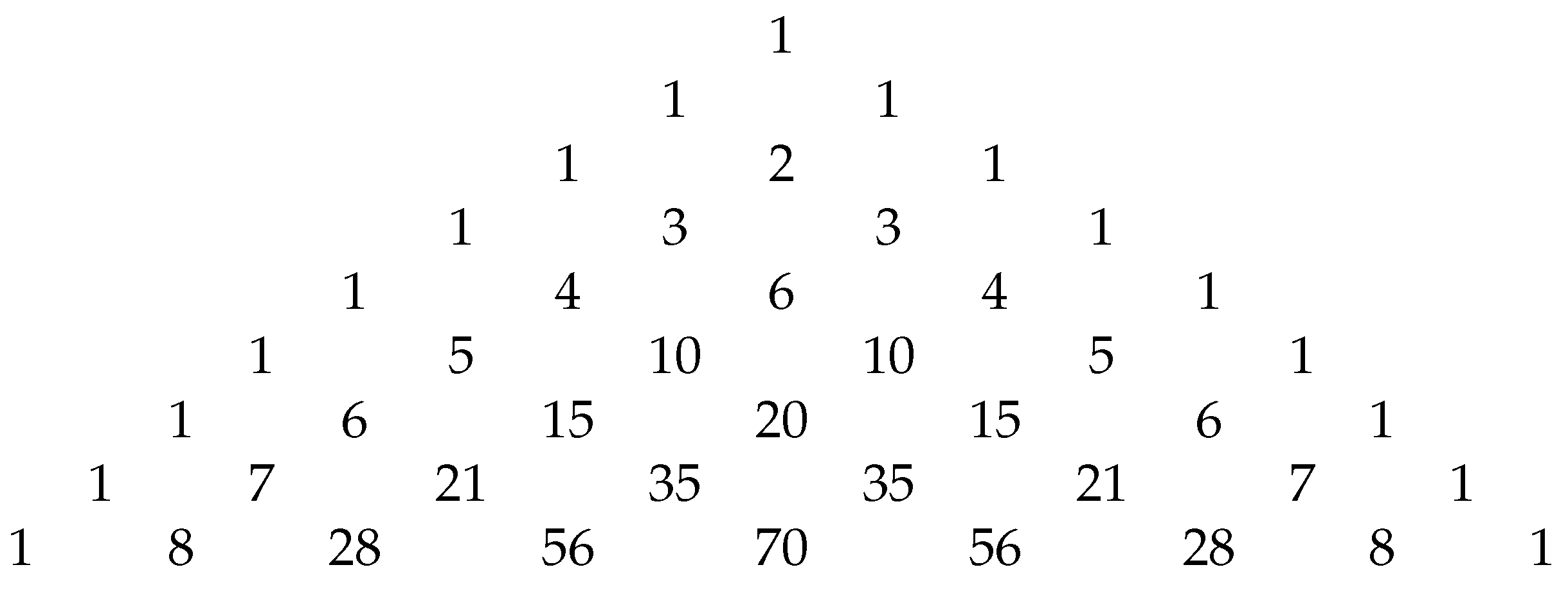
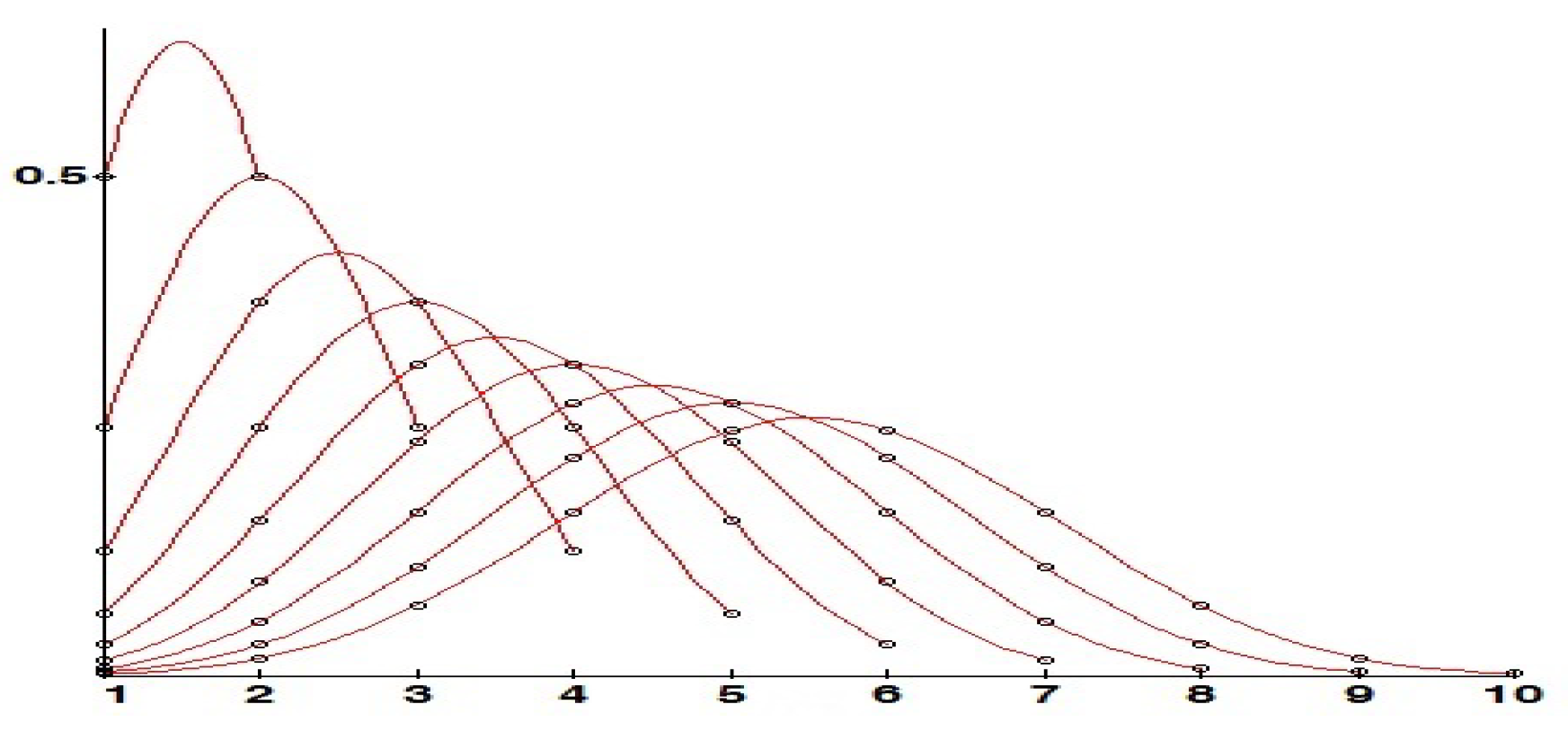
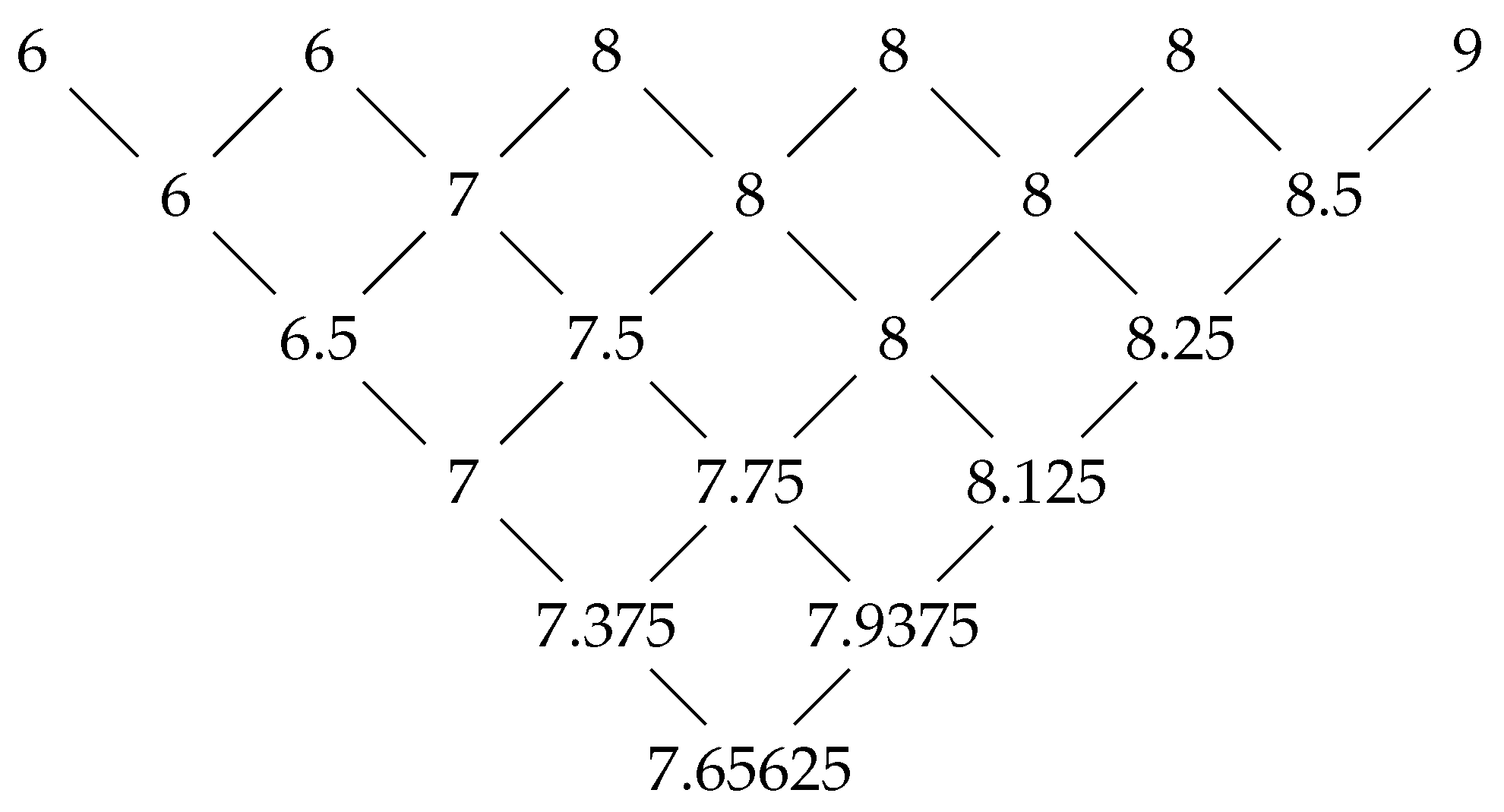
3. Binomial OWA Rules

Let $n\ge 1$ and

$$p_i^n=\left(\genfrac{}{}{0pt}{}{n-1}{i-1}\right)\mathrm{for}\mathrm{all}i=1,2,\cdots ,n$$

(3)

which are well-defined for each positive integer n. A well-known property of Pascal’s numbers in (3) is ${\displaystyle \sum _{i=1}^n}{p}_i^n=2^{n-1}$ for all positive integer n. For each $a\in (0,1)$, consider the weights

$$w_i^n=p_i^n·a^{i-1}·{(1-a)}^{n-i}$$

(4)

These weights define for each $a\in (0,1)$ an OWA binomial rule of dimension n,12]. The binomial term is due to the following probabilistic interpretation of the coefficients. The weights of $w_i^n$ follow a binomial distribution X with parameters $n-1$ (which stands for the number of trials) and $p=a$ (which stands for the probability of success), so that

$$w_i^n=P(X=i-1)$$

for $i=1,\cdots ,n$, which is approximated by the normal distribution with parameters:

$$\mu =(n-1)aand\sigma =\sqrt{(n-1)·a·(1-a)}.$$

(5)

An interesting particular case arises when $a=1/2$. Then, (4) becomes $w_i^n:=q_i^n$ where

$$q_i^n=\frac{p_i^n}{2^{n-1}}$$

(6)

and the normal approximation in (5) has parameters:

$$\mu =\frac{n-1}{2}and\sigma =\frac{\sqrt{n-1}}{2}.$$

(7)

Henceforth, I refer to the binomial OWA rule for $a=\frac{1}{2}$ as the F-rule, which can be expressed as:

$$F^n(x_1,\cdots ,x_n)=\sum _{i=1}^n{q}_i^n·x_i$$

Figure 1 shows the numerators $p_i^n$ in (3) of the weighted coefficients $q_i^n$ in (6) of the F-rule for small values of n. These numbers form the well-known Pascal triangle. As the number of judges is known in advance, I just need to take the numbers $p_i^n$ in the nth row in Figure 1 and standardize them to get the weights $q_i^n$ for F. For instance, the numbers in the antepenultimate row are used to calculate the F-rule for a panel of seven judges. Figure 2 shows the shapes of bidimensional graphics $(i,q_i^n)$ of $F^n$-rules for panels of $n=2,\cdots ,10$ judges:

Variants of the F-Rule

In this subsection, I introduce variants of the F-rule, based on discarded extreme judges’ scores, similarly to the trimmed versions of the mean, $M_{-1}^{-1}$ and $M_{-2}^{-2}$.

The F-rule minus the best and the worst judges’ scores for $n\ge 3$: I just remove $x_1$ and $x_n$ in (2), redefine the scores $x_i$ for $i>1$ and $i<n$ as $x_i:=x_{i+1}$, replace n by $n-2$ and then apply the F-rule to the new $n-2$ variables. That is, I take

$$F^{n-2}(x_1,\cdots ,x_{n-2})={\displaystyle \frac{1}{2^{n-3}}}\sum _{i=1}^{n-2}{p}_i^{n-2}·x_i=\sum _{i=1}^{n-2}{q}_i^{n-2}·x_i$$

(8)

Hereafter, I refer to the OWA in (8) as $F_{-1}^{-1}$.

The F-rule minus the two best and the two worst judges’ scores for $n\ge 5$: I just remove $x_1$, $x_2$, $x_{n-1}$ and $x_n$ in (2), redefine the scores $x_i$ for $i>2$ and $i<n-1$ as $x_i:=x_{i+2}$, replace n by $n-4$ and then apply the F-rule to the new $n-4$ variables. That is, I take

$$F^{n-4}(x_1,\cdots ,x_{n-4})={\displaystyle \frac{1}{2^{n-5}}}\sum _{i=1}^{n-4}{p}_i^{n-4}·x_i=\sum _{i=1}^{n-4}{q}_i^{n-4}·x_i$$

(9)

Hereafter, I refer to the OWA in (9) as $F_{-2}^{-2}$.

The numerators of the coefficients $q_i^{n-2}$ and $q_i^{n-4}$ to compute the $F_{-1}^{-1}$ and $F_{-2}^{-2}$ indices, respectively, appear in Figure 1. As the number of judges is fixed and known in advance, I just need to take the respective numbers in the $(n-2)$th and $(n-4)$th row in Figure 1. For instance, the numbers in the fifth row are used to calculate the $F_{-1}^{-1}$-rule for a panel of seven judges and to calculate $F_{-2}^{-2}$-rule for a panel of nine judges.

4. Some Characterizations of the F-Rule

4.1. A Characterization as a Binomial Rule

It is clear that the binomial rules satisfy monotonicity and strict monotonicity, as described in Section 2, since positivity, $w_i^n>0$ for all n and $i\le n$ in (4), implies strict monotonicity by Proposition 1. The next result concerns the properties of symmetry and ID-monotonicity of binomial rules.

Proposition 2.

• A binomial rule is symmetric if and only if $a=\frac{1}{2}$.
• A binomial rule is ID-monotonic for n large enough if and only if $a=\frac{1}{2}$.

Proof. 

• The converse is clear since

  $$\left(\genfrac{}{}{0pt}{}{n-1}{i-1}\right)=p_i^n=p_{n-i+1}^n=\left(\genfrac{}{}{0pt}{}{n-1}{n-i}\right)$$

  for all $i\le n$, which implies $q_i^n=q_{n-i+1}^n$. For the direct implication, assume that the binomial rule is symmetric, then $w_i^n=w_{n-i+1}^n$ for all $i=1,2,\cdots ,n$, which implies $p_i^n{a}^{i-1}{(1-a)}^{n-i}=p_{n-i-1}^n{a}^{n-i}{(1-a)}^{i-1}$. Thus, $a=1-a$ and $a=\frac{1}{2}$.
• The converse is clear since

  $$\begin{array}{ccc}\left(\genfrac{}{}{0pt}{}{n-1}{i-1}\right)<\left(\genfrac{}{}{0pt}{}{n-1}{i}\right)& \mathrm{if}& i=1,\cdots ,\lceil \frac{n}{2}\rceil -1,\mathrm{and}\\ \\ \left(\genfrac{}{}{0pt}{}{n-1}{i-1}\right)>\left(\genfrac{}{}{0pt}{}{n-1}{i}\right)& \mathrm{if}& i=\lfloor \frac{n}{2}\rfloor +1,\cdots ,n-1.\end{array}$$

  which, respectively, imply $q_i^n<q_{i+1}^n$ if $i=1,\cdots ,\lceil \frac{n}{2}\rceil -1$ and $q_i^n>q_{i+1}^n$ if $i=\lfloor \frac{n}{2}\rfloor +1,\cdots ,n-1$.
  For the direct implication, I assume that the binomial rule is not the F-rule, i.e., $a\ne \frac{1}{2}$.
  Assume first that $a>\frac{1}{2}$ and n is odd. Consider

  $$\frac{w_{\frac{n+1}{2}}^n}{w_{\frac{n+3}{2}}^n}=\frac{n+1}{n-1}·\frac{1-a}{a}$$
  As $\frac{1-a}{a}<1$ is a fixed number and $\underset{n\to \infty }{lim}\frac{n+1}{n-1}=1$ there exists some $n_0\in \mathbb{N}$ such that for all $n\ge n_0$, it holds that $w_{\frac{n+1}{2}}^n<w_{\frac{n+3}{2}}^n$, which ensures that ID-monotonicity fails. The proof for $a>\frac{1}{2}$ and n even is analogous to the former one by checking that $w_{\frac{n}{2}+1}^n<w_{\frac{n}{2}+2}^n$ for n large enough, which ensures that ID-monotonicity fails.
  The proof for $a<\frac{1}{2}$ is analogous to the previous one by checking, in the odd case, that $w_{\frac{n+1}{2}}^n<w_{\frac{n-1}{2}}^n$ for n large enough, and that $w_{\frac{n}{2}}^n<w_{\frac{n}{2}-1}^n$ for n large enough, inequalities that lead to failures of ID-monotonicity.

□

Proposition 2 highlights the F-rule, since it is the only OWA based on the binomial distribution which satisfies symmetry and ID-monotonicity. The probabilistic interpretation of the binomial rules together with one of these two properties constitute a characterization of the F-rule.

Corollary 1.

• The F-rule is the only binomial rule which satisfies symmetry.
• The F-rule is the only binomial rule which satisfies ID-monotonicity.

The F-rule, in contrast to rules M and D, has other interesting properties deduced from the structure of its weights. These two additional properties follow from known properties of the binomial distribution.

The central concavity ($CC$-property):

A sequence of OWAs, ${\left\{G^n\right\}}_{n\ge 1}$, satisfies the CC-property if the pairs $(i,w_i^n)$ are either concave in the domain of indices or concave in a central interval of the domain of indices and convex in two extreme intervals.

The bidimensional graphic of the pairs $(i,q_i^n)$ for $i=1,\cdots ,n$ has the next pattern: for $n\le 5$ it is concave, for $n\ge 6$ it is convex on the left of the domain of indices and on the right of it, while concave in the middle. This property is fulfilled by the sequence of rules ${\left\{F^n\right\}}_{n\ge 1}$ because Pascal’s numbers verify it. Observe, for example, in Figure 2 that for $n=9$, concavity is achieved in the interval $[3,7]$, while convexity is achieved in $[1,4]\cup [6,9]$. Thus, the two inflection points in the normal approximation with parameters given in (7) and shown in Figure 2 belong to the real intervals $(3,4)$ and $(6,7)$.

The interquartile asymptotic density (asymptotic $IQ$-density):Let $IQ$ be the interquartile interval of judges’ scores in (2), i.e., the interval between the first and third quartiles. A sequence of OWAs, ${\left\{G^n\right\}}_{n\ge 1}$, satisfies the asymptotic IQ-density if:

$$\underset{n\to \infty }{lim}\sum _{i:x_i\in IQ}{w}_i^n=1.$$

This property is fulfilled by the sequence of rules ${\left\{F^n\right\}}_{n\ge 1}$ and its proof is easily derived from the normal approximation in (7) of the binomial distribution.

4.2. A Characterization as an OWA Rule

Let $n\ge 2$ be the number of judges and $\Gamma$ be a closed and bounded real interval. From the ordered judges’ grades $x=(x_1,\cdots ,x_n)$ $x_1\le x_2\le \cdots \le x_n$, consider $y=(y_1,\cdots ,y_{n-1})$ such that $y_i=\frac{x_i+x_{i+1}}{2}$ for all $i=1,\cdots ,n-1$, which obviously satisfy $y_1\le y_2\le \cdots \le y_{n-1}$ and $y_i\in \Gamma$ for all $i=1,\cdots ,n-1$. I say that y is the average reduction of x.

A sequence of OWAs ${\left\{G^n\right\}}_{n\ge 1}$ satisfies the invariant average reduction (IAR) if $G^n\left(x\right)=G^{n-1}\left(y\right)$ for all $n\ge 2$ and whenever y is the average reduction of x.

Vector y is a way of shrinking vector x, keeping the value of the rule invariant. By successively shrinking vector x, the value of the rule is obtained. From a practical perspective, this axiom is compelling: a rule satisfying the IAR can be viewed as transparent, as it can be computed by a recursive procedure of means of consecutive pairs of scores.

Proposition 3.

A sequence of OWAs ${\left\{G^n\right\}}_{n\ge 1}$ satisfies the IAR if and only if it is the sequence of ${\left\{F^n\right\}}_{n\ge 1}$-rules.

Proof. 

The sequence of $F^j$-rules for all $j\le n$ satisfies the IAR, since $q_i^n+q_{i-1}^n=q_i^{n+1}$ for all $i=1,\cdots ,n-1$, which is a consequence of the well-known property of Pascal’s numbers:

$$\left(\genfrac{}{}{0pt}{}{n}{i}\right)=\left(\genfrac{}{}{0pt}{}{n-1}{i-1}\right)+\left(\genfrac{}{}{0pt}{}{n-1}{i}\right),$$

(10)

For the converse, I proceed by induction on the number of judges.

Let $n=2$, by the IAR, it holds

$$w_1^2{x}_1+w_2^2{x}_2=w_1^1{y}_1=w_1^1\left(\frac{x_1+x_2}{2}\right)$$

The OWA conditions for $n=1$ and $n=2$ imply $w_1^1=1$ and $w_2^2=1-w_1^2$. Thus,

$$\left(\frac{1}{2}-w_1^2\right)(x_1-x_2)=0$$

(11)

Let $\chi =(z_1,z_2)$ be a vector such that $z_1<z_2$; by substituting it in (11) it follows that $w_1^2=\frac{1}{2}$. Hence, $w_1^2=w_2^2=\frac{1}{2}$.

Assume the condition is true for all n, i.e.,

$$w_i^n=\frac{\left(\genfrac{}{}{0pt}{}{n-1}{i-1}\right)}{2^{n-1}}i=1,\cdots ,n$$

I want to see that

$$w_i^{n+1}=\frac{\left(\genfrac{}{}{0pt}{}{n}{i-1}\right)}{2^n}i=1,\cdots ,n+1$$

By the IAR, it holds

$$\sum _{i=1}^{n+1}{w}_i^{n+1}{x}_i=\sum _{i=1}^n{w}_i^n{y}_i$$

By the definition of the $y_i$’s, the induction hypothesis, the well-known property of Pascal’s numbers (10) for all $i=1,\cdots n-1$ and using $\left(\genfrac{}{}{0pt}{}{j}{0}\right)=\left(\genfrac{}{}{0pt}{}{j}{j}\right)=1$ for all positive integer j, it holds:

$$\sum _{i=1}^{n+1}{w}_i^{n+1}{x}_i=\frac{1}{2^n}\left[\sum _{i=1}^{n+1}\left(\genfrac{}{}{0pt}{}{n}{i-1}\right)x_i\right]$$

Thus,

$$\sum _{i=1}^{n+1}\left(w_i^{n+1}-\frac{1}{2^n}\left(\genfrac{}{}{0pt}{}{n}{i-1}\right)\right)x_i=0$$

(12)

Equation (12) can be written as

$$\sum _{i=1}^{n+1}{c}_i{x}_i=0$$

(13)

where $c_i=w_i^{n+1}-\frac{1}{2^n}\left(\genfrac{}{}{0pt}{}{n}{i-1}\right)$. Let $\Gamma =[a,b]$. To prove that $c_i=0$ for all i, consider the vectors ${\chi }^j$ for $j=1,\cdots ,n+1$ satisfying (2) and with the j largest components equal to b and the rest of the components (for $j\le n$) equal to a. By applying (13) to these $n+1$ vectors, it results for all $j=1,\cdots ,n+1$:

$$C·{\chi }^j=0$$

(14)

where $C=(c_1,\cdots ,c_{n+1})$ and “·” is the inner product.

From (14) it follows an homogeneous and linear system with unknowns $c_i$ and unique solution $c_i=0$ for all $i=1,\cdots ,n+1$. Thus,

$$w_i^{n+1}=\frac{\left(\genfrac{}{}{0pt}{}{n}{i-1}\right)}{2^n}i=1,\cdots ,n+1.$$

as desired. □

5. Other Significant Advantages of Using the $\mathbf{F}$-Rule

As seen in the previous sections, several mathematical properties support the use of the F-rule. In this section I still want to emphasize other desirable properties, in a slightly more informal way, that a good rule should ideally fulfill.

These new properties refer to: discrimination, outliers’ dependency, consistency with respect to truncations of the rule itself, and computational simplicity.

5.1. Discrimination

Assume there is a large number of candidates m. Let n be the number of judges on the panel and assume that the domain of the judges’ scores is $\Gamma =\{0,1,\cdots ,10\}$. Then, each judge has 11 choices between 0 and 10 and the F-rule is either 10 or a rational number between 0 and 9, plus a fraction of the type $i/2^{n-1}$ where $i=0,1,\cdots ,2^{n-1}-1$. Thus, the range of values for the F-rule is $10·2^{n-1}+1$. This number is considerably high, even for moderately small panels, and guarantees very few ties among candidates.

By way of comparison, I consider the range for the mean, M-rule, under the same assumptions. The M-rule is either 10 or a number between 0 and 9, plus a fraction of the type $i/n$ where $i=0,1,\cdots ,n-1$. Thus, the range of values for the mean is $10·n+1$. This number is considerably smaller than $10·2^{n-1}+1$, even for panels of a reduced number of judges. Therefore, ties among candidates are much more frequent for the M-rule than for the F-rule. Of course, the lack of discrimination is even more pronounced for the median, the D-rule, which is the main drawback of the median as a good rule for evaluating candidates.

5.2. Almost Independence of Extreme Judges’ Scores

Judges’ scores in the interquartile interval are the most transparent evaluation of the candidates’ performances. Scores in the interquartile interval are the only ones that are surely free of outliers (i.e., extreme scores produced for some personal technical reason or, even, for manipulation) and therefore should be of greater importance in the rule selected. The interquartile range, the difference between the third and the first quartiles, is a good measure of dispersion for skewed distributions. Outliers for technical reasons should be minimized, whereas outliers for manipulation should ideally be avoided.

As reflected by the asymptotic $IQ$-density, the F-rule for a moderate number of judges mainly depends on the central grades, so the incidence of extreme scores is minimal when F or any other of its variants, $F_{-1}^{-1}$ or $F_{-2}^{-2}$, are used. Oppositely, the dependency on judges’ extreme scores of the M-rule and its variants is high.

The F-rule cannot prevent manipulation, since results in [13,14,15,16] fail for it, but at least it minimizes its incidence. The larger the panel of judges, the less manipulable the F-rule is. The variants $F_{-1}^{-1}$ and $F_{-2}^{-2}$ rules prevent the manipulation of a few judges and preserve the main ideas of F.

5.3. Almost Consistency with Its Variants

Assume there are at least two candidates, $m\ge 2$. Let x and y be the scores obtained by two candidates, which are taken orderly as in (2). I write $G\left(x\right)$ for the aggregated evaluation for the OWA G. Let H be another OWA. A reversal of two candidates with scores x and y for the pair of OWAs G and H arises when

$$\left(G\right(x)-G(y\left)\right)·\left(H\right(x)-H(y\left)\right)<0.$$

This means that G and H order x and y oppositely.

The interest here lies in the reversals of an OWA with its variants. For instance, between the M-rule and any of its variants $M_{-1}^{-1}$ or $M_{-2}^{-2}$, or between the F-rule and any of its variants $F_{-1}^{-1}$ or $F_{-2}^{-2}$. If $M\left(x\right)-M\left(y\right)>0$ and $M_{-1}^{-1}\left(x\right)-M_{-1}^{-1}\left(y\right)<0$, then I say that the rules M and $M_{-1}^{-1}$reverse candidates’ scores x and y. The same applies for F and its variants $F_{-1}^{-1}$ and $F_{-2}^{-2}$.

If $M\left(x\right)-M\left(y\right)\ne 0$ and is close to zero, then the x’s and y’s outliers become decisive in whether M and $M_{-1}^{-1}$ or M and $M_{-2}^{-2}$ show reversals. I regard this situation as an internal inconsistency of the rule M since it reflects that it is vulnerable to some small score changes. Reversals are seen as an internal weakness. I claim that the mean witnesses many reversals, which is another reason to discard it as a good aggregating rule since M, $M_{-1}^{-1}$ and $M_{-2}^{-2}$ easily provide different rankings.

Fewer reversals are observed for F and $F_{-1}^{-1}$ or for F and $F_{-2}^{-2}$. The intuition lies in the fact that F and its variants are very little dependent on extreme scores in comparison with the M rule and its variants. Simulations for a particular sports event, see [17], showed that reversals of F with its variants were very infrequent.

5.4. Computational Simplicity

The F-rule is an OWA, so it is very simple to be understood and computed by the audience, in contrast with some sophisticated rules that are applied in some sports. The IAR property illustrates that the F-rule can be calculated iteratively by just computing $\frac{n(n-1)}{2}$ means of pairs of numbers, which is incredibly easy.

Figure 3 shows this iterative calculation of a candidate with grades $(6,6,8,8,8,9)$, which was evaluated by a panel of six judges. The numbers in the second row in Figure 3 are the means of the indicated numbers in the first row. The numbers in the remaining rows are obtained in the same way. Thus, the F-rule is $F(6,6,8,8,8,9)=7.65625$.

6. Conclusions

OWAs constitute a large family of aggregation rules. The mean, the median and some trimmed means are examples of OWAs that are frequently used in practice and are supported for several theoretical works. This article proposes an alternative which, as far as I known, is new and is supported by several theoretical arguments exposed in the previous sections. By way of summary, I review here some of its good properties:

• It is based on the binomial (and normal) distribution;
• It is sensitive to an increase or decrease of any judge’s score;
• It is representative of the panel of judges; all judges’ scores count;
• It discriminates very well and ties among candidates are almost avoided;
• It mostly concentrates the aggregated score in the intermediate judges’ scores, and this tendency increases when the number of members in the panel increases;
• It is consistent with its variants $F_{-1}^{-1}$ or $F_{-2}^{-2}$, so that reversals are almost nonexistent;
• It has very little dependence on extreme judges’ scores; although potential judges’ manipulation is not fully avoided, at least it is considerably minimized when compared with other rules such as the mean;
• Close versions $F_{-1}^{-1}$ or $F_{-2}^{-2}$ can prevent having a few manipulators or radical judges, while keeping almost all the ideas that support F; the hypothetical presence of manipulators or radical judges may suggest the use of one of these two variants;
• It is also useful to evaluate the post judges’ reliability. A way to do that is by summing the coefficients $q_i^n$ assigned by the judge to all the candidates being evaluated. Judges who are poorly scored in this way can be potentially penalized;
• It is transparent, very simple to compute and therefore easy to be understood for candidates and potential audience;
• It has been shown to be applicable as a tie-breaking system in open tournaments with a limited number of rounds and many participants, e.g., as in chess, go, scrabble, bridge, etc., see [17].

We highlighted the median, the mean and some trimmed means, among the most relevant studied alternative aggregation rules to the one proposed in this paper. Note that the median and close rules to it, such as the majority judgment, fail to be representative and do not discriminate well, resulting in many draws (properties 3, 4 and 11 above fail for the median). The mean and some of its trimmed versions show a worst behavior than the F-rule for properties 4 to 8 and 11. Moreover, the median and the mean rules do not satisfy strict $ID$-monotonicity, the $CC$-property and the asymptotic $IQ$-density.

The main motivation of the present article was to propose a simple and well-defined rule that could be implemented in practice in multiple real-life situations that require aggregation. It would be of great interest if the proposal were analyzed in detail by other scholars. Theoretical studies on the proposed rule would be of interest, such as, for example, obtaining a compelling new axiomatic characterization of the F-rule. Carrying out simulations to verify the intuitively high degree of fulfillment of the properties stated in Section 5.2 and Section 5.3 is also a topic of interest. As stated, the F-rule is not immune to manipulation, and studies on this issue would also be significant. Finally, I wonder whether it exists a rule, not coming from a discretization of a normal distribution, that satisfies the properties for an OWA stated in Section 2 as well as the $CC$-property and the asymptotic $IQ$-density in Section 4.

References

1. Hillinger, C. The case for utilitarian voting. Homo Oeconomicus 2005, 23, 295–321. [Google Scholar] [CrossRef] [Green Version]
2. Macé, A. Voting with evaluations: Characterizations of evaluative voting and range voting. J. Math. Econ. 2018, 79, 10–17. [Google Scholar] [CrossRef]
3. Balinski, M.L.; Laraki, R. Majority Judgement: Measuring, Ranking, and Electing; The MIT Press: Cambridge, MA, USA, 2011. [Google Scholar]
4. Aleskerov, F.; Chistyakov, V.V.; Kalyagin, V. The threshold aggregation. Econ. Lett. 2010, 107, 261–262. [Google Scholar] [CrossRef]
5. Carlsson, C.; Fullér, R.; Fullér, S. OWA operators for doctoral student selection problem. In The Ordered Weighted Average Operators: Theory and Applications; Yager, R.R., Kacprzyk, J., Eds.; Kluwer Academic Publishers: London, UK, 1997; pp. 167–177. [Google Scholar]
6. Crowley, L. The best average: It’s time to change how we compute scores. Int. Gymnast. 2002, 44, 34. [Google Scholar]
7. Gambarelli, G. The ‘coherent majority average’ for juries’ evaluation processes. J. Sport. Sci. 2008, 26, 1091–1095. [Google Scholar] [CrossRef] [PubMed]
8. Technical Regulations 2022. Fédération Internationale de Gymnastique. Available online: https://www.gymnastics.sport/site/ (accessed on 19 October 2022).
9. Csiszar, O. Ordered weighted averaging operators: A short review. IEEE Syst. Man, Cybern. Mag. 2021, 7, 4–12. [Google Scholar] [CrossRef]
10. Yager, R.R. On ordered weighted averaging aggregation operators in multicriteria decision making. IEEE Trans. Syst. Man Cybern. 1988, 18, 183–190. [Google Scholar] [CrossRef]
11. Yager, R.R.; Kacprzyk, J. The Ordered Weighted Averaging Operators, Theory and Applications; Kluwer Academic Publishers: London, UK, 1997. [Google Scholar]
12. Montero, J.; Cutello, V. Aggregation rules in committee procedures. In The Ordered Weighted Average Operators: Theory and Applications; Yager, R.R., Kacprzyk, J., Eds.; Kluwer Academic Publishers: London, UK, 1997; pp. 219–237. [Google Scholar]
13. Freixas, J.; Parker, C. Manipulation in games with multiple levels of output. J. Math. Econ. 2015, 61, 144–151. [Google Scholar] [CrossRef] [Green Version]
14. Gibbard, A. Manipulation of voting schemes: A general result. Econometrica 1973, 41, 587–601. [Google Scholar] [CrossRef] [Green Version]
15. Moulin, H. On strategy-proofness and single peakedness. Econometrica 1980, 35, 437–455. [Google Scholar] [CrossRef]
16. Satterthwaite, M.A. Strategy-proofness and Arrow’s conditions: Existence and correspondence theorems for voting procedures and social welfare functions. J. Econ. Theory 1975, 10, 187–217. [Google Scholar] [CrossRef]
17. Freixas, J. The decline of the Buchholz tiebreaker system: A preferable alternative. In Transactions on Computational Collective Intelligence, vol. XXXVII. Lecture Notes on Computer Science, 13750; Nguyen, N.T., Kowalczyk, R., Mercik, J., Motylska-Kuźma, A., Eds.; Springer: Berlin/Heidelberg, Germany, 2022. [Google Scholar]
Figure 1. The numbers of Pascal’s triangle, p i n for all n = 1 , , 9 and i = 0 , , n 1 .
Mathematics 10 04418 g001
Figure 2. Weights q i n for the F n -rules from n = 2 to n = 10 .
Mathematics 10 04418 g002
Figure 3. Recursive method to compute the F-rule by just using means of pairs of numbers.
Mathematics 10 04418 g003
Publisher’s Note: MDPI stays neutral with regard to jurisdictional claims in published maps and institutional affiliations.