Mathematical Chemistry Approaches for Computer-Aid Design of Free-Shaped Structures in Architecture and Construction Engineering

Abstract

The use of computers in architecture and construction engineering simplifies and automatize many manual operations, especially in the case of curved surfaces such as shell structures. Moreover, it allows fast screening and characterization of many technical solutions through computer-solving equations and the verification of buildings and metallic structures stabilities in different weather and seismic conditions. In parallel, significant efforts have been made to characterize and explore carbon-based nanosystems. Important mathematical concepts and methods were developed for the description of such structures in the frame of mathematical chemistry. Because the lattice topology of shell structures in architecture and nanosystems in chemistry are similar, it is possible to transfer well-established theoretical concepts and knowledge of using nanosystems to the design of shell structures. The topologies of the nanosystems are characterized by lower densities of edges per node offering better solutions for curved surfaces than the typical grids used in architecture. As far as we know, no such connections between the topologies of nanosystems and shell structures have been established before. This transfer would be helpful for increased accuracy and speed in finding the best technical solutions for the building’s design. In this paper, we identify and propose for the design of the shell structures several mathematical approaches developed for atomistic systems.

1. Introduction

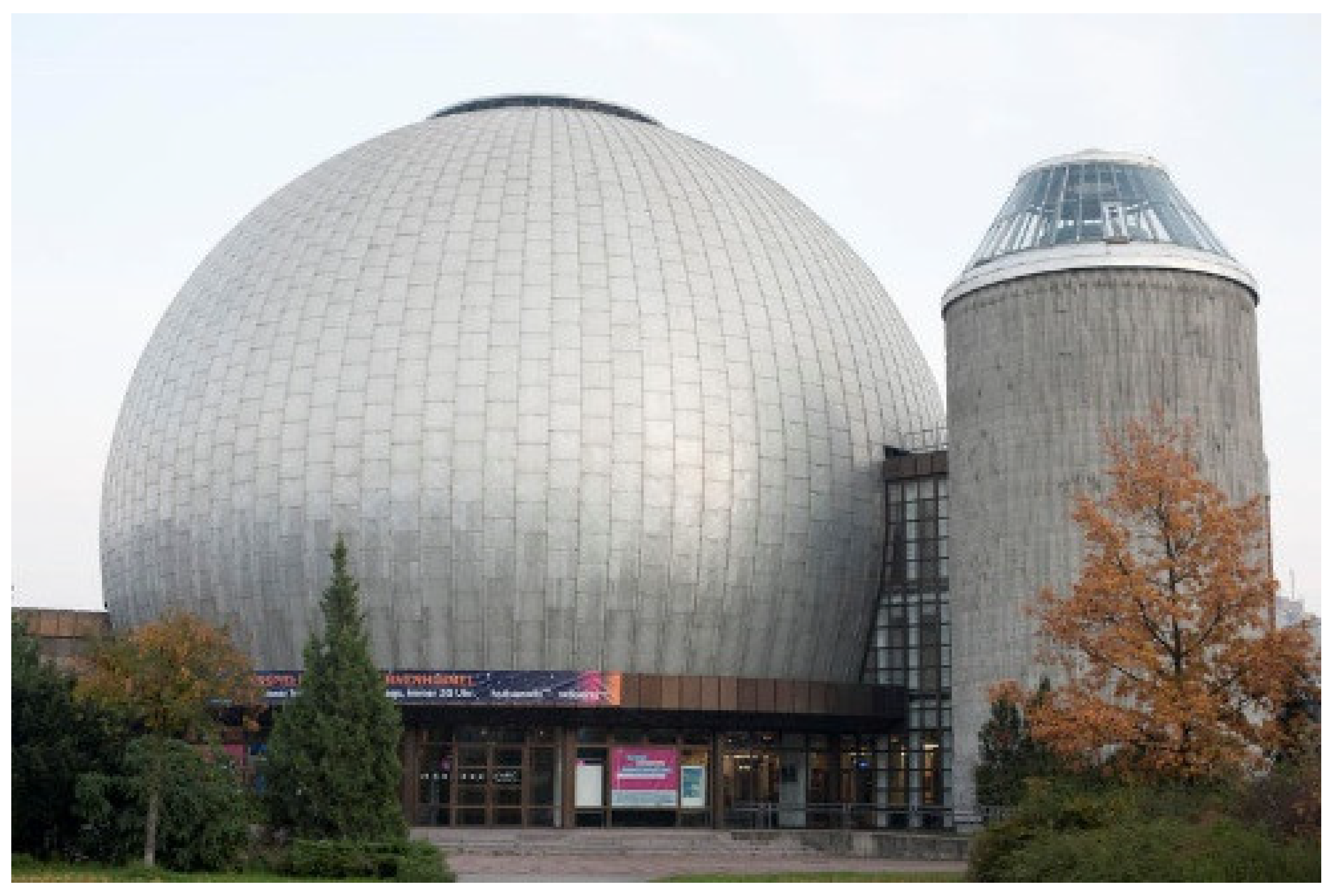
Modern architecture uses more and more polyhedral platonic geometric forms and curved surfaces together with traditional orthogonal shapes. The curved surfaces, characterized by bended, curled and twisted curves, can be designed as more interesting and pleasantly shapes, with a high degree of continuity. The most representative curved surface is the geodesic dome, which is a hemispherical shell structure based on supported and self-supported triangular, quadrilateral, or hexagonal lattices. In 1919, Walther Wilhelm Johannes Bauersfeld designed the first building with an icosahedron shape, a planetarium for the company Carl Zeiss, in Berlin, Germany (see Figure 1). Richard Buckminster Fuller, a prolific architect and engineer, continued to popularize this technology as a building design. He introduced the term of the geodesic dome.

The three-dimensional curved surfaces, called shell structures, have one dimension much smaller than the other two and are constructed from panels of various shapes. Some beams along the edges of the panels give resistance to the structure against the external loads. The panel shapes and the size of the beams are designed in such a way as to reduce the bending moments and structure compression. The connected beams that form a shell structure define a grid or mesh. The beams are arranged along the edges of the grids. The alternative way to describe a grid is to define the connection points of beams, called nodes of the grid.

The 3D curved surface is discretized on a 3D grid with simple predefined mesh topologies, such as triangular, quadrahedral, pentagonal and hexagonal lattices [2]. The structured meshes with implicit connectivity are the most familiar and simple. In the most general form, the triangular grids are unstructured. The triangular grids can be easily automated and have important benefits for numerical treatments. However, they encompass a high density of edges and high connectivity of the grid nodes (of the order of six edges connected to a node). The implementations of non-triangular grids are numerically more efficient and provide less density, superior transparency and greater design freedom. They can be obtained by merging of few triangular rings of the grids. The exterior edges of the triangles that share a node (called the central node) can be considered as a larger ring of a new grid. The size of the new ring is equal to the connectivity of the corresponding central node. Thus, for planar grids four- and six-member rings are formed, but for non-planar grids, other ring sizes are also determined.

The quadrilateral mesh has four coordinating nodes. Quadrilateral grids are compatible with planar or regular shapes (cylinders, cones). The hexagonal grids involve less coordination of the node to 3. However, it is more appropriate for the planar or cylindrical meshes and requires to be deformed for the spheroidal or ellipsoid shapes. Pentagonal grids give the sphericity and concave shapes, and the heptagonal and octagonal grids generate objects with a convex shape.

For the mechanical (structural stability and deformation) characterization of the shell structure under external forces, a further discretization (or meshing) of the beams and nodes is required for the Finite Elements Model (FEM) simulations, which make calculations for a limited number of points and interpolate the results for the entire surface or volume.

Several mathematical tools were developed in the field of architecture. Geometry computing is the field of mathematics that has been developed and applied to freeform architecture, by computer design, surface discretization on grids with the help of the Bezier curves, and calculation at points extra grid nodes by Non-uniform rational basis spline (NURBS). Building Information Modelling (BIM) is the digital integrated technique that integrates and simplifies the collaboration and data management of the architecture, engineering and construction industries. BIM identifies the technical solutions that have to balance the constraints of the engineering (material properties, technological solutions) and financial (cost, sustainability, maintenance) aspects. Several computer graphics and computer-aided design applications—CAD software (ArchiCAD [3], Blender [4], Grasshopper [5], Rhino 3D [6] and SketchUp [7], just to enumerate a few of them) are available for the design of free-form surfaces and the characterization of the shell structures for architectural and interior modeling and industrial design. FEM can further use the designed shell structures by meshing free-form surfaces and characterize the stability of the shell structures under various external factors (wind, rain, snow, ice, shocks and vibrations) based on the static and dynamic linear-elastic stress analysis (Ansys [8], Autodesck [9], AutoFEM [10], Catia [11], Dlubal [12], FreeCAD [13], KiCAD [14], OpenFOAM [15], PyCAD [16] and SolidWORKS [17]). Thus, the overuse of construction materials and disasters can be avoided by predicting the minimal size of the beams and nodes in order to control the stress below the values of the breaking thresholds, in order to avoid construction collapse.

Mathematical chemistry is a subfield of mathematics, which provides the theoretical framework and methodology for the various fields of chemistry [18,19,20,21]. In particular, different fields of mathematical chemistry (chemistry graph theory, algorithms of structure enumeration and generation, molecular static and dynamic methods) were developed, parameterized and applied to the investigation of various structures formed by carbons atoms. At the nanoscale the carbon atoms form two-dimensional lattices, which are characterized by five- and six-member rings, where carbon atoms are connected to another three neighbor carbons atoms by strong covalent bonds. The topologies of these nanosystems are very similar to those of the macroscopic shell structures but have fewer edges per node and implicitly more reduced self-weight.

In the present paper, we transfer some knowledge to architecture and construction engineering and mathematical tools developed by materials science researchers in their approaches to the nanostructures formed by atoms. Section 2 is dedicated to the description of the problematics of the nanostructures, especially those formed by the carbon atoms (tube-like, cones, junctions and fullerenes) and to some mathematical tools developed for their characterization (graphs, topologies, Schlegel diagram, Hamilton and spiral paths, enumeration and building algorithms). Various carbon-based nanosystems are presented and their topology is discussed from the perspective of building algorithms. In Section 3 we suggest the transfer of some mathematical tools developed for nanosystems to the shell structures based on five- and six-member rings. The design of five- and six-ring shell structures to an imposed ground contour is presented. A calculation scheme is suggested. A modified Elastic Network Model is proposed as a particle-based dynamic simulation method. The possibilities of using various software for the transferring of the nanosystem models to the macroscale and discretization for the Finite Element Method simulations are suggested.

2. Carbon Nanoscale Structures

Carbon presents many allotropes, with the most known natural structures as crystals, diamond (the carbon atoms form a three-dimensional 3D crystalline lattice) and graphite (the carbon atoms are stacked on hexagonal lattices on two-dimensional sheets), or amorphous materials (the carbon atoms fill the three-dimensional, without regular arrangements) [22,23,24]. These systems are compact and extended and are built by carbon atoms that are mostly connected in a hybridization sp³, sp² or mixed, respectively. Many other 3D compact carbon structures are predicted to be stable by molecular simulations [25,26].

The carbon atoms might also form limited-size allotropes, where each atom is arranged in a two-dimensional hexagonal-type lattice, similar to the graphite layer, called graphene [27,28]. The graphene sheets can be folded in such a way to form differently shaped nano-objects [29] as tubes [30], tori and foams.

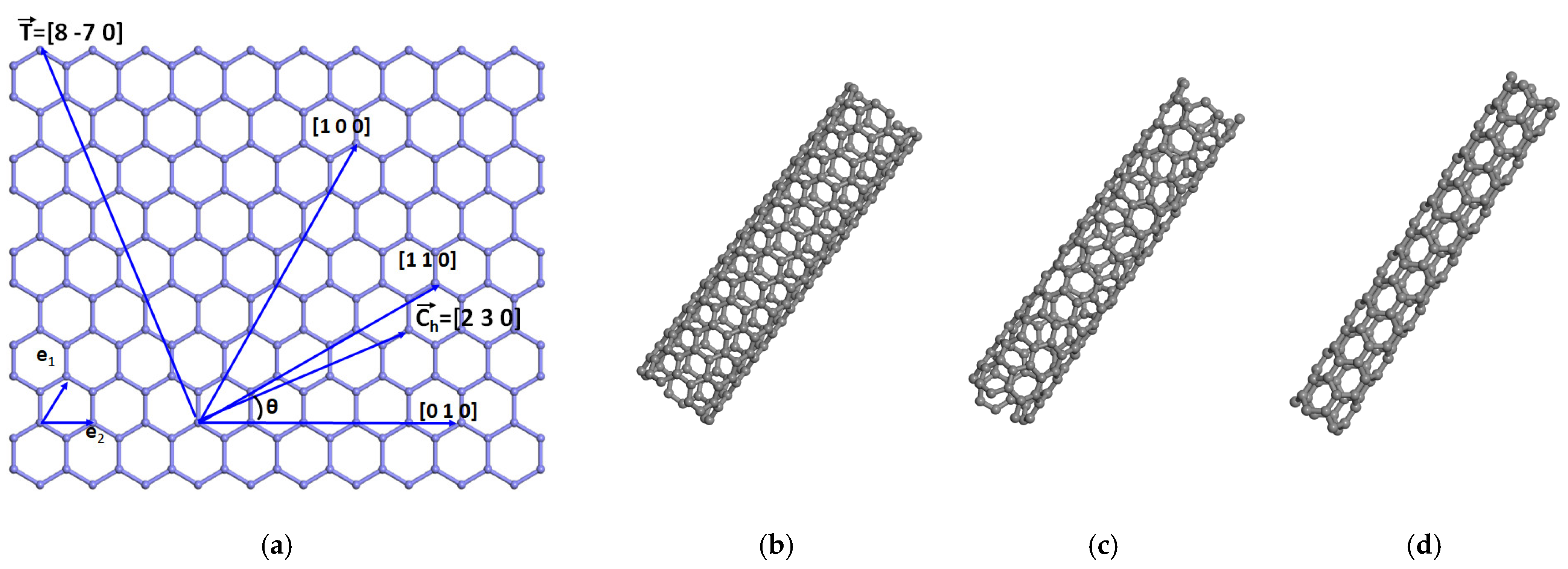
A single-wall carbon nanotube can be built by rolling up a hexagonal lattice (graphene or a layer of graphite) [31], along the chiral vector

$${\overrightarrow{C}}_h=n{\overrightarrow{e}}_1+m{\overrightarrow{e}}_2\equiv (n,m),\hspace{1em}n,m\in \mathbb{Z}$$

(1)

where ${\overrightarrow{e}}_1=\frac{a}{2}\left(\sqrt{3},1\right)$, and ${\overrightarrow{e}}_2=\frac{a}{2}\left(\sqrt{3},-1\right)$ (see Figure 2a) are the vectors that describe the hexagonal lattice, of length $a=\left|{\overrightarrow{e}}_1\right|=\left|{\overrightarrow{e}}_2\right|=l\sqrt{3}$, with l as the internode distance. n and m are any integer numbers. A nanotube of diameter $d=\frac{a}{\pi }\sqrt{n^2+nm+m^2}$ is obtained by rolling the planar hexagonal sheet along the vector

$$\overrightarrow{T}=h{\overrightarrow{a}}_1+k{\overrightarrow{a}}_2\equiv (h,k),\hspace{1em}h,k\in \mathbb{Z}$$

(2)

where $h=\left(2m+n\right)/\delta$ and $k=-\left(2n+m\right)/\delta$ are integer numbers determined by n and m in such a way that $\overrightarrow{T}$ is orthogonal to ${\overrightarrow{C}}_h$. $\delta$ is the greatest common integer divisor of integers $2n+m$ and $n+2m$. The number of hexagonal rings in the nanotube is $N=2(n^2+nm+m^2)/\delta$.

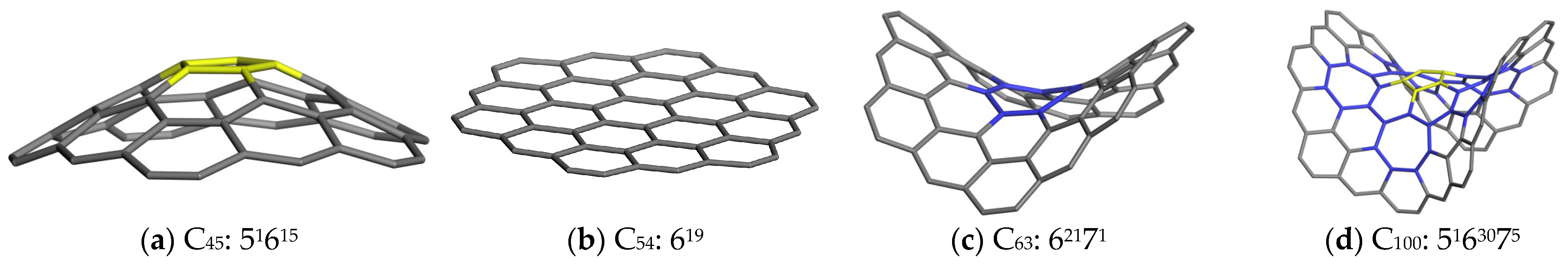
The hexagonal lattice is a 2D planar lattice of hexagonal rings, sharing a common edge with their neighboring rings. The existence of five and/or seven-member rings such as in some carbon flakes makes the system nonplanar (see Figure 3a–d).

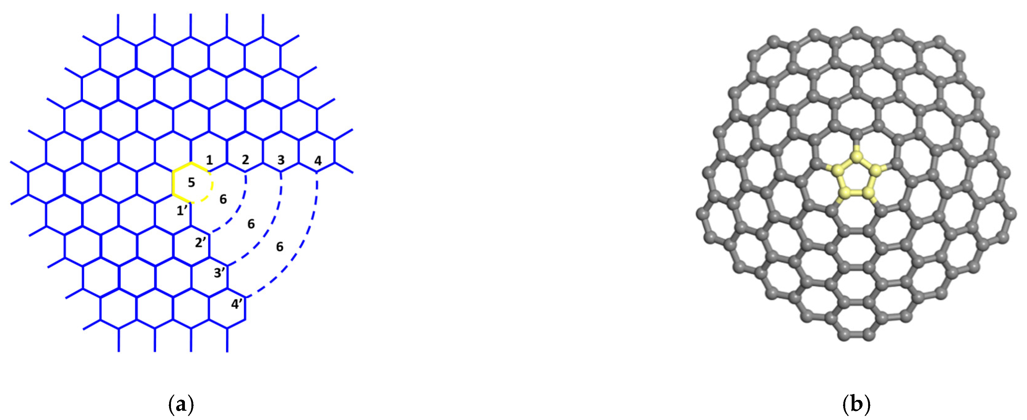
Nanocones are formed when one or a few pentagonal rings are inserted in the middle of a graphene piece [32,33]. Topologically, such cones can be derived from a hexagonal lattice (see Figure 4a), where a sixth region is removed and the non-three-coordinated atoms are bond-connected (dash lines in Figure 4a) [34]. The central ring becomes a five-member ring (see Figure 4b).

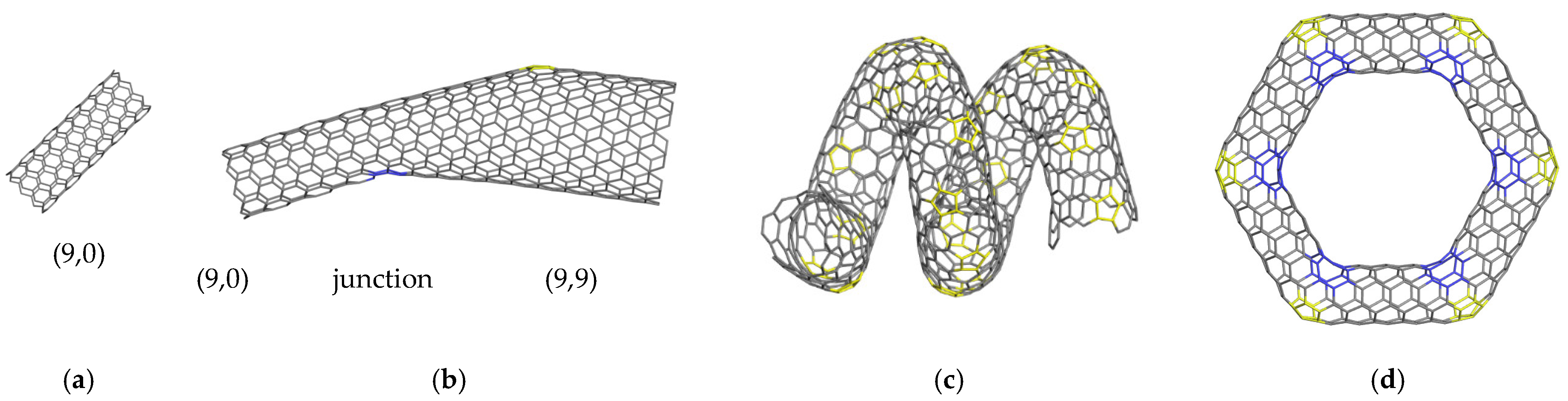
The nanotubes obtained from rolled graphite sheets (see, for example, Figure 5a) are monodimensional systems, but they can be transformed into three-dimensional systems by introducing several non-hexagonal rings. Thus, two nanotubes of different chirality types can be joined by introducing pentagonal and hexagonal rings. In Figure 5b, a hetero-junction between two nanotubes (9,0) and (9,9) is shown; there is a heptagonal ring at the boundary between the (9,0) nanotube and the heterojunction, and a pentagonal ring at the boundary between (9,9) and the heterojunction. When several successive pentagonal rings are inserted into a nanotube, it transforms into a nano-spiral system (see Figure 5c), or into a closed torus (see Figure 5d), when several heptagonal rings are also considered.

When the carbon atoms form 12 pentagons that share their edges with none or additional hexagonal rings cage-type structures C_n, named fullerenes, are formed. The first discovered fullerene is C₆₀ [37], formed by n = 60 carbon atoms arranged on a sphere and called Buckminsterfullerene after the name of Richard Buckminster Fuller. Except for n = 22, a fullerene can be formed by any number of carbon atoms n ≥ 20. 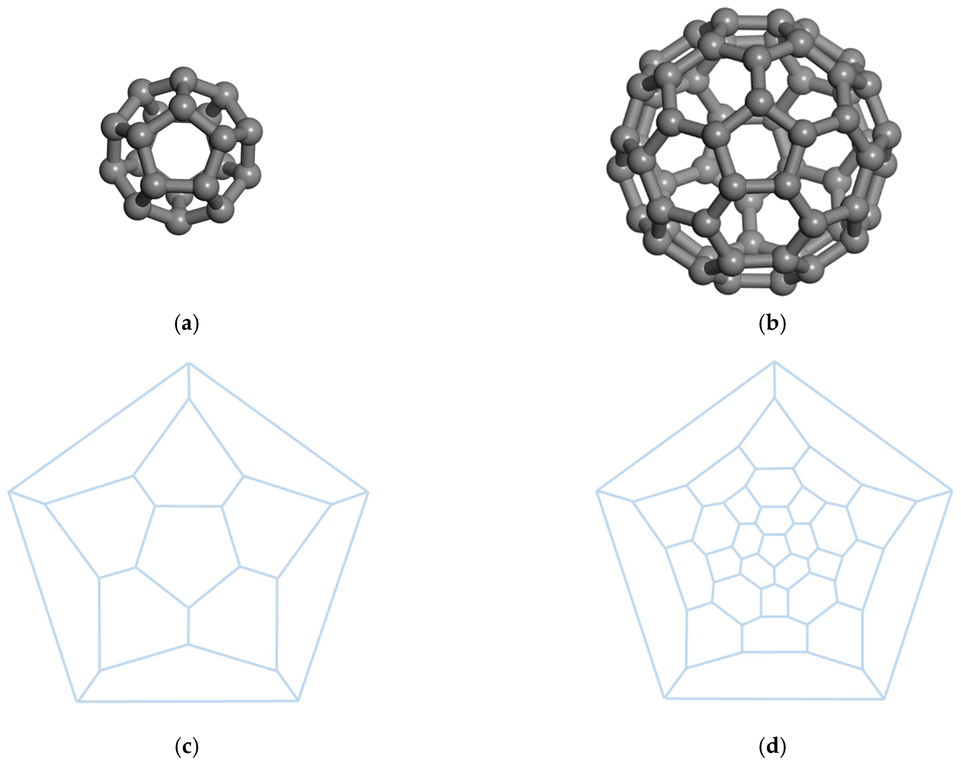The C₂₂ contains four-member rings or even seven-member rings depending on how the pentagons are arranged [38]. The fullerenes with only five- and six-member rings are called classical fullerenes, or just fullerenes. The fullerenes that also contain other types of rings are called extended or non-classical fullerenes. In Figure 6, two spherical fullerenes C₂₀ and C₆₀, are shown.

The topology of the polyhedrons is analyzed by graph theory (a subfield of discrete mathematics) that analyses the pairwise connectivity of the connected structures. Thus, a graph is a set G = (V, E), where V are the vertices (occupied by atoms or molecules) and E are the edges (pairs of atoms or molecules) [39]. A fullerene is a three-regular graph (each node is connected to the other three nodes) with faces that are five or six in size. From each vertex (the carbon atoms) three edges start (the bond between two carbon atoms), and each edge is shared by two rings. Therefore, a fullerene C_n made by n carbon atoms has $n_E=3/2n$ edges. Since every edge is determined by the intersection of two faces, the number of edges is $n_E=(5n_P+6n_H)/2$, where $n_P$ and $n_H$ are the number of pentagonal and hexagonal rings, respectively. Based on the Euler theorem for the convex polyhedrons $n_F+n=n_E+2$, where $n_F=n_P+n_H$ is the total number of faces. Thus, the number of pentagonal and hexagonal faces can be determined as $n_P=12$ and $n_H=n/2-10$. There is a huge number of possible arrangements for the pentagonal and hexagonal rings, estimated at $n^9$, each case corresponding to an isomer of C_n [40].

The connectivity of the nodes in the graph is described by a matrix called the connection matrix. The elements have a value of 1 when the rows and columns correspond to connected nodes, and a value of 0 when the respective nodes are not connected. The dual graph, defined by the central points of the rings, is a triangular graph. The number of vertices, edges, and faces of the dual graph is equal to the number of rings, edges, and vertices of the initial graph, respectively [41].

The distinction between two isomers of C_n can be made by their symmetry or by the determinant of the connectivity matrix that describes the topology of the fullerenes [42]. Another tool provided by graph theory is the Schlegel diagrams [43], a method for reducing the representation of fullerene to a two-dimensional graph that describes the connectivity of the nodes on the graph and the arrangement of the rings (see Figure 6c,d).

The smallest fullerene, C₂₀, has a spherical shape and consists only of 12 pentagons, no hexagons, and has 30 edges (see Figure 5a). The arrangement of the $n_P=12$ pentagonal and $n_H=20$ hexagonal rings of C₆₀ is the same as in the case of the standard soccer-ball polyhedron and has 90 edges (see Figure 5b). The pentagonal and hexagonal rings can also be arranged in various orders, yielding a variety of 1812 isomers but being less stable than buckminsterfullerene. The most stable fullerene satisfies the so-called isolated pentagonal rule (IPR), which states that two pentagonal rings must not share an edge [44]. The explanation of IPR is that a pentagonal ring is surrounded by five hexagonal rings, reducing the strain energy. Any other isomer of C₆₀ has at least a pair of pentagonal rings that share one edge. It is shown that the complementary units (CU), which are the pieces of the carbon network remaining after the removal of the pentagonal rings from the structure [45], stabilize the isomers of C₈₄. The CUs lead the planar area and the adjacent pentagons induce the sphericity of the fullerenes and increase the strain energy.

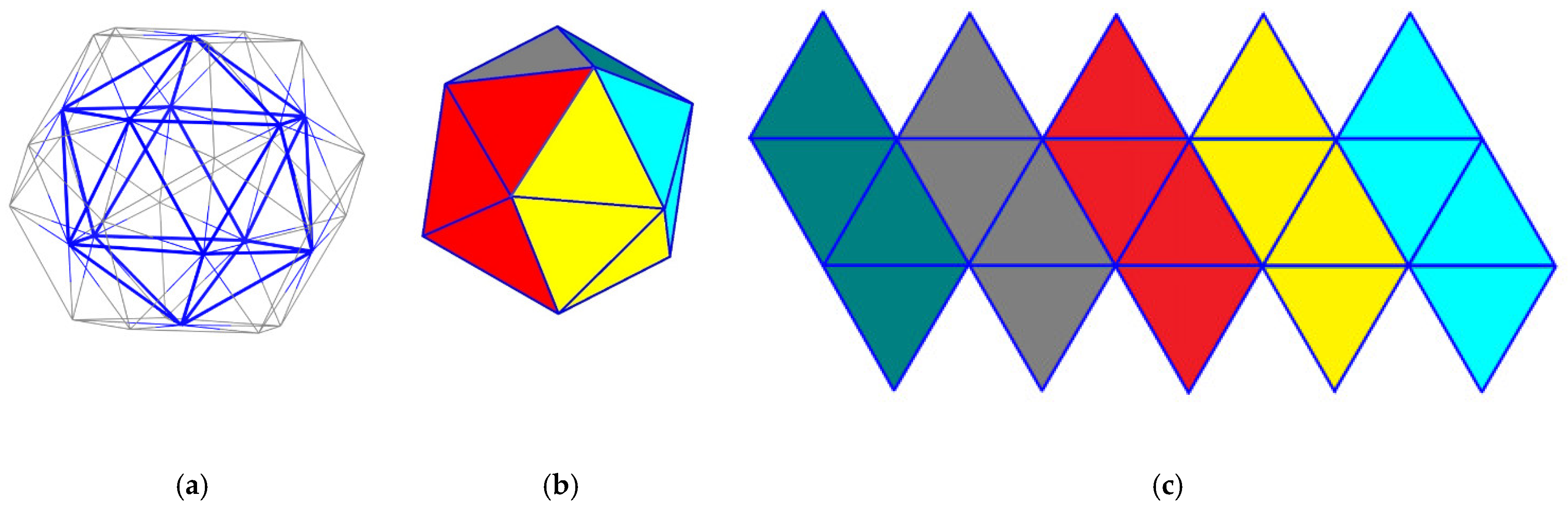
Considering the centers of the pentagonal rings and connecting them, we obtain the dual graph of the dodecahedron, which is the icosahedron, a polyhedron with 20 triangle faces (see Figure 7a) [46]. The vertices of the icosahedron have a degree of 5. After coloring each of the three neighboring faces of an icosahedron with the same color (Figure 7b), the unfolded icosahedron looks like Figure 7c.

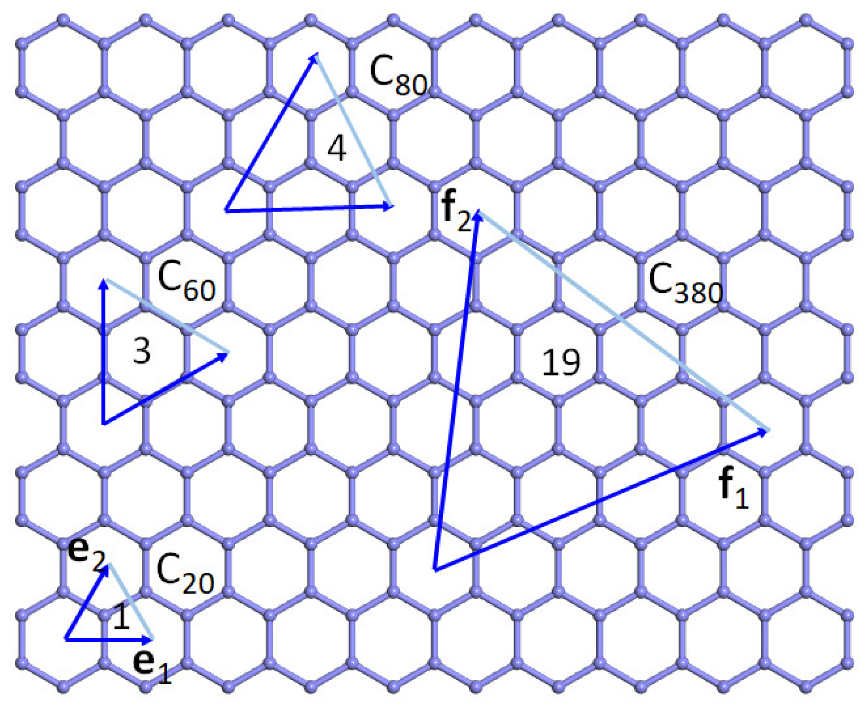
By decorating the equilateral triangle faces with an equilateral triangle cut from the carbon hexagonal lattice (see Figure 8), we can produce the Schlegel diagrams for the fullerenes of different sizes with the highest symmetry, the icosahedral one. These isomers are among the most stable fullerenes, as the pentagons are at the largest distances.

The pentagons are formed at the sites of the 12 sets of crossing tree triangles, and the other rings are hexagons, with a number of fullerene vertices of (m² + mn + n²), where m and n are integer numbers that determine the orientation of the equilateral triangle.

$${\overrightarrow{f}}_1=m{\overrightarrow{e}}_1+n{\overrightarrow{e}}_2,{\overrightarrow{f}}_2=-n{\overrightarrow{e}}_1+(m+n){\overrightarrow{e}}_2,\hspace{1em}n,m\in \mathbb{Z}$$

(3)

and ${\overrightarrow{e}}_1$ and ${\overrightarrow{e}}_2$ are the vectors of the hexagonal lattice (see Figure 8).

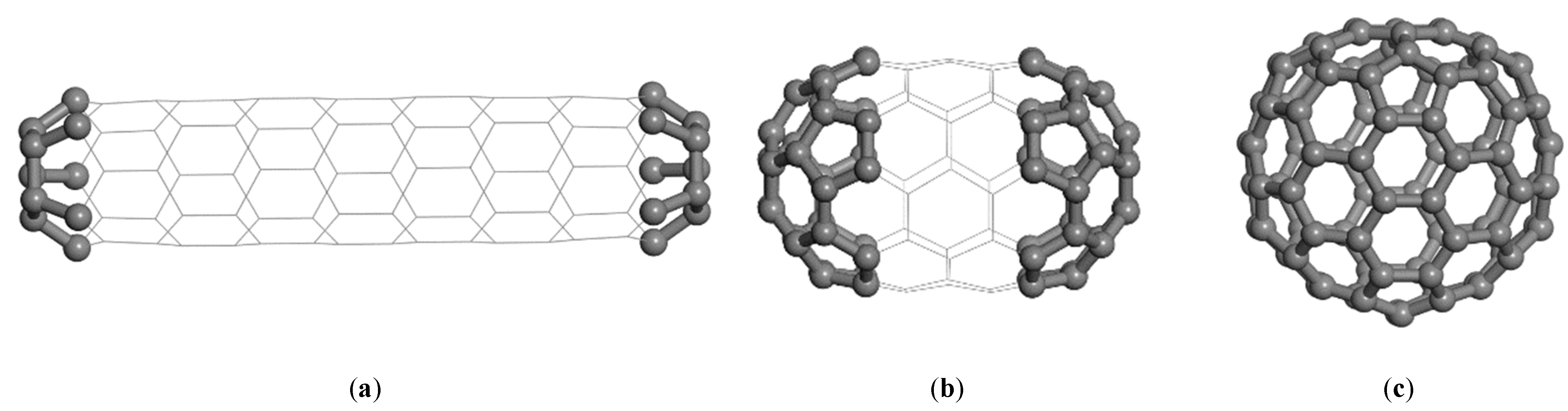
Depending on how the five- and six-membered rings are arranged, different isomers can be constructed for a given order n. In Figure 9, three isomers of C₉₀ are presented as examples. The first two isomers (see Figure 9a,b), with an oblong shape and a symmetry of C_5h, are actually capped nanotubes of type (5,0) and (5,5) with two halves of C₂₀ and C₆₀ at the ends, respectively. A round-shaped fullerene with the symmetry C_2v is presented in Figure 9c. Any nanotube can be capped with half of a fullerene. Therefore, such nanotubes are also called cylindrical fullerenes. The capped nanotubes are less stable because of the high curvature at the ends of the nanotubes. A nanotube decorated by dispersed pentagons may have a spiral shape, depending on the distribution of the pentagonal rings.

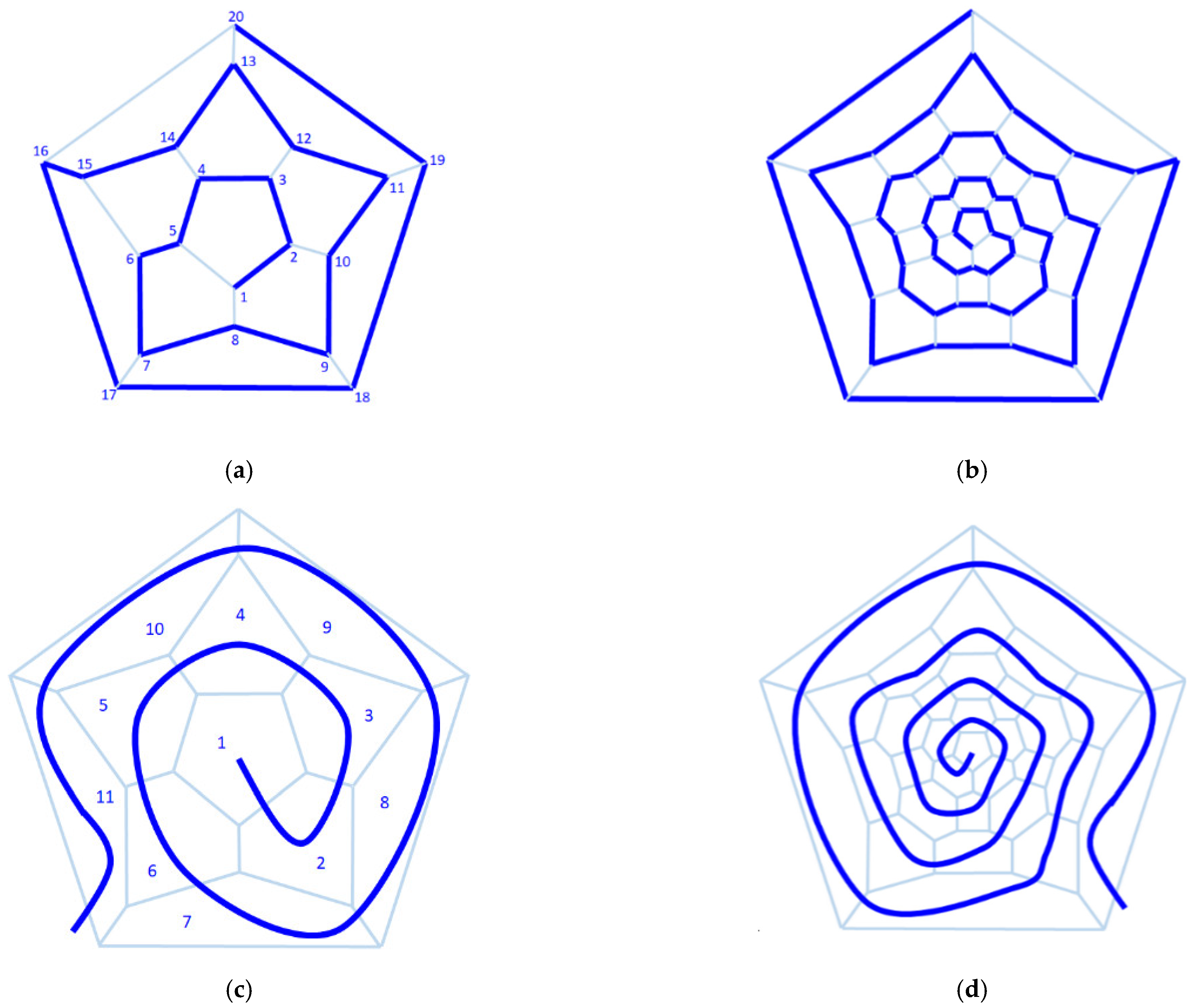
How can the arrangement of the rings be described? The solution is provided by graph theory, which defines the Hamilton path as a path that begins at one face (usually a pentagonal one) and proceeds in a spiral order through each face that is visited exactly once [47,48]. A similar path can be determined by using the vertices as references instead of the faces. When the path ends at the same initial face or vertex, the Hamiltonian path is called the Hamiltonian cycle. In the first row of Figure 10 are presented the Hamiltonian paths for C₂₀ and C₆₀ fullerenes, the smallest fullerenes with the icosahedral symmetry Ih. The numbering of the nodes is along the Hamilton path. Thus, based on the ordering of the types of rings, the different isomers can be distinguished and the unique isomers are identified.

The spiral path can be used for the generation of all the isomers of C_n in the so-called spiral algorithm [49], which specifies the positions of the pentagons along the spiral path. For fullerenes larger than n = 380, there are a few cases of isomers that cannot be generated by this algorithm [50]. Software can generate the 3D isomers of fullerenes: Buckygen [51], AME [52], CaGe [53], Fullgen [54], Fui-GUI [55] and Fullerene [56]. These codes differ by implementation, performance and completeness of the sets of isomers, and some of them generate both the 3D structure and the Schlegel diagram.

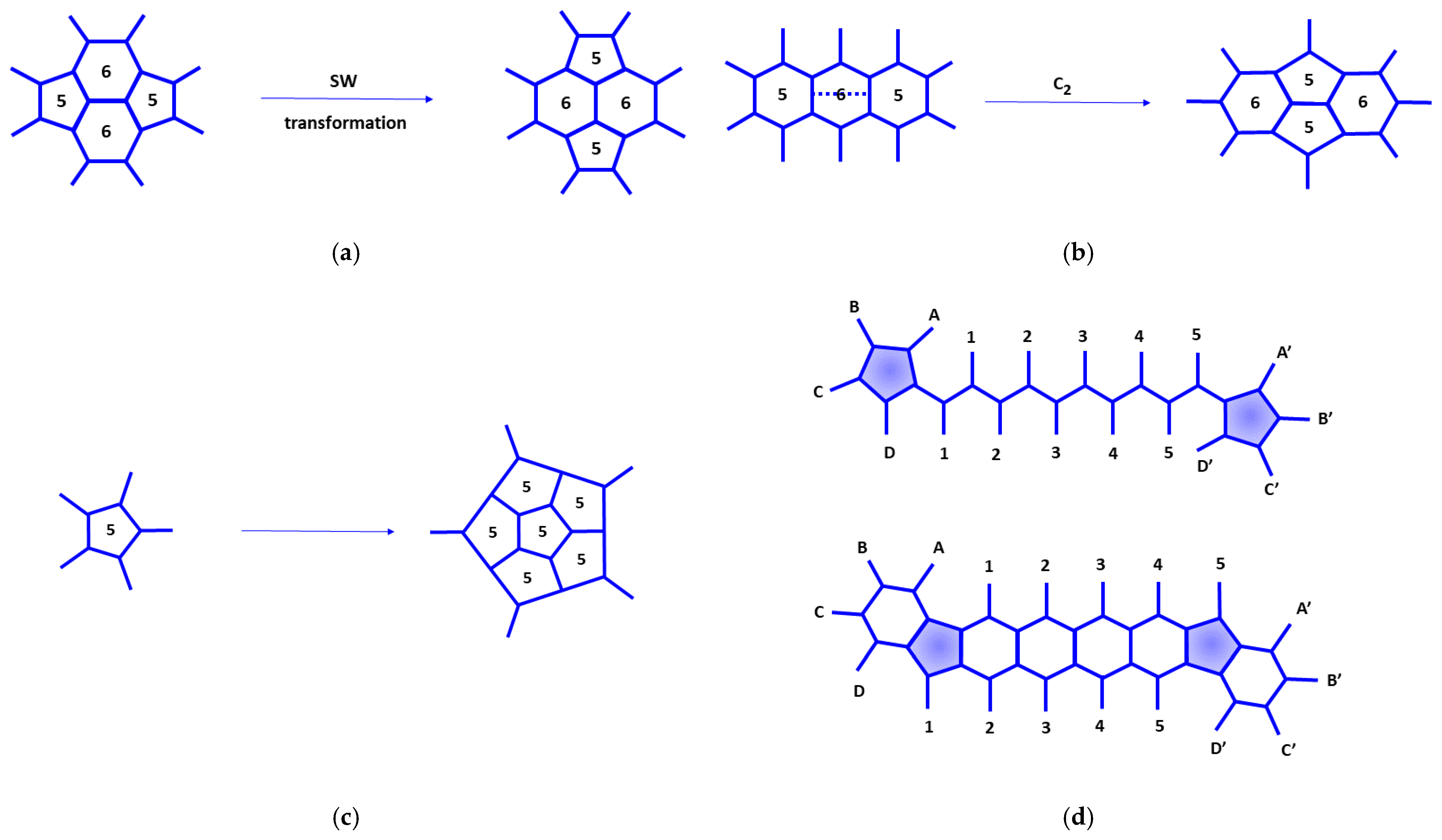
The isomers can be transformed from one to another by the Stone–Wales rearrangements [57], which consist of the rotation of a common edge of two pentagonal rings by 90° (see Figure 11a). Some rings different from five and six-member rings, which are considered defects, are produced for other situations. Larger fullerenes can be constructed from a given fullerene by insertion of a dimer C₂ into a hexagonal ring connected to two pentagonal rings (the Endo–Kroto procedure [58], see Figure 11b) or insertion of pentagonal and hexagonal rings (see Figure 11c,d). Thus, the connectivity of the respective rings with the environmental atoms is preserved. Fullerene coalescence [59] is another growth mechanism that can be described at the atomic scale [60].

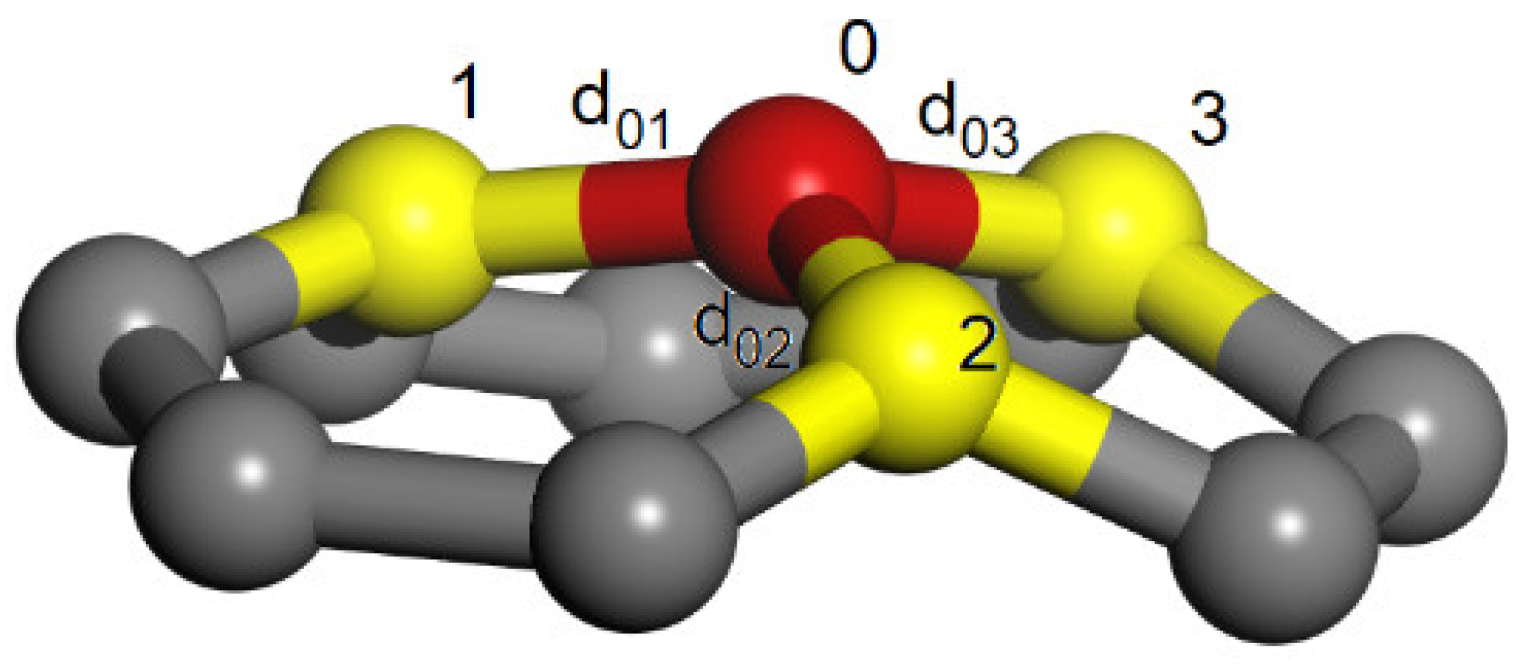
For a given Schlegel diagram or connectivity matrix, with specified internode distances, the coordinates of the nodes can be determined by the distance geometry algorithms [61,62,63]. The procedure is capable to give the Cartesian coordinates of the fourth vertex (denoted by the index 0 in Figure 12) with desired distances from the other three neighbor vertices 1–3 which for the Cartesian coordinates are already determined. In order to satisfy all the internode demanded distances the algorithm can be iteratively applied for all the nodes. An alternative procedure for a known Schlegel diagram consists of successive assembling of the rings, which have edges of lengths corresponding to the desired internode distances. The procedure starts with three assembled rings that share one node and continue by adding rings of appropriate size along the spiral path.

3. Applications to Architecture and Construction Engineering

The concepts and mathematical methods presented in the previous section are very useful for the design of shell structures with topologies characterized by three-coordinated nodes, as in the case of the carbon nanosystems. The linear, spiral, and junction tube-like substructures can be used as connection elements and supporting poles for shell structures. The fullerene and cone curved-type structures can be used as components of the shell structures. The transformation procedures presented in Figure 11 can be used for the redesign of shell structures in order to control the shape of the shell and the uniform distribution of the mechanical tension along the shell, for structure stabilization.

For a fixed contour of the grid shell on the ground, a patch of compatible fullerene can be chosen. A procedure for the completion of the fullerene piece with the given contour, as for the filling curve, can be applied by inserting new vertices and flipping edges to obtain a triangulation [64]. Depending on the density of these triangles near the contour and their topology, the triangular patches are merged into a coarse-grained grid of pentagons and hexagons, and occasionally other types of cycles. To control stress within the grid vertices network, nodes are displaced in space to ensure specific inter-vertices distances. The beams that are oriented along the edges of the fullerene-type structure form the shell structure.

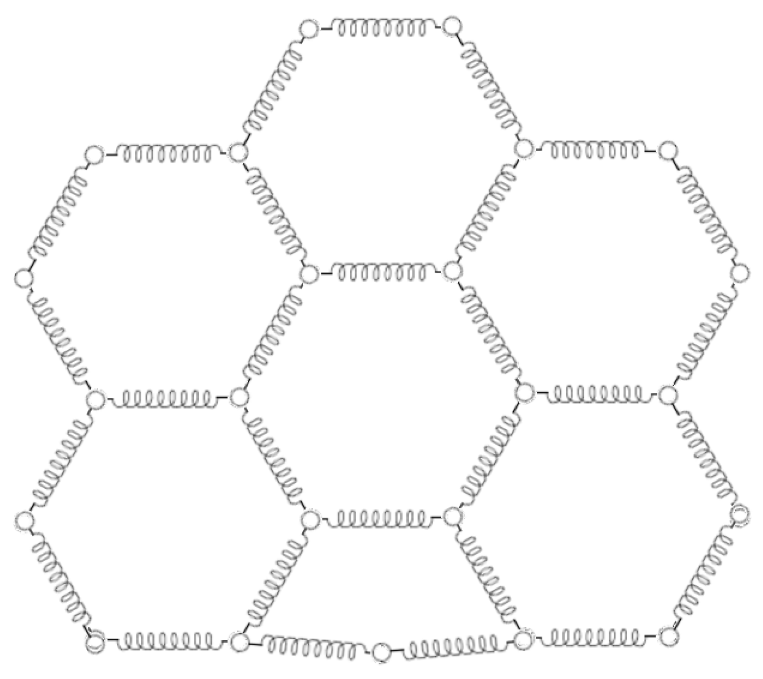
The fullerene-type shell structures can be treated in terms of a very simple particle-based model such as the Elastic Network Model (ENM), where the nodes of the structure are represented by particles that interact through elastic forces [65,66] along the grid edges (see Figure 13). ENM was developed as a simulation tool for the study of protein flexibility by coarse-graining the vibrational normal modes. It reduces the computational effort by replacing the interatomic force calculation with a simple elastic interaction [67,68]. Thus, the elastic energy of the shell structure is

$$E_{elast}={{\displaystyle \sum _{i<j=1}^N{\gamma }_{ij}\left(\left|{\overrightarrow{r}}_{ij}\right|-d_{ij}\right)}}^2$$

(4)

where N is the total number of nodes, ${\gamma }_{ij}$ and $d_{ij}$ are the elastic constants and the length of the beam that connect the nodes i and j, $\left|{\overrightarrow{r}}_{ij}\right|$ is the current distance between the nodes i and j. The parameter $\left|{\overrightarrow{r}}_{ij}\right|-d_{ij}$ represents the deviation from the length of the beam. The deformation strain or longitudinal strain of the edge i–j is defined as ${\epsilon }_{ij}=\frac{\left|{\overrightarrow{r}}_{ij}\right|-d_{ij}}{d_{ij}}$ and it has negative and positive values indicating the beam contraction and elongation, respectively. In our model, we consider only the elastic deformation of the beams. For the case of plastic deformation, the Finite Element Method has to be applied.

The ENM has to be modified by applying some external forces (gravitation, mass of the deposited ice or dust on the shell, waves induced by wind, rain or earthquakes) on nodes. The ground-supported particles are considered solidly fixed to the support and follow its motion due to the waves generated by earthquakes or soil motion such as sliding by the interaction energy

$$E(\left|{\overrightarrow{r}}_i-{\overrightarrow{r}}_{i\perp }\right|)=\left\{\begin{array}{c}\infty ,\hspace{1em}\hspace{1em}\hspace{1em}\hspace{1em}\hspace{1em}\hspace{1em}\hspace{0.33em}\hspace{0.17em}\left|{\overrightarrow{r}}_i-{\overrightarrow{r}}_{i\perp }\right|\ge 2d_{i0}\\ {{\displaystyle \sum _{i<j=1}^N{\gamma }_{i0}\left(\left|{\overrightarrow{r}}_{i0}\right|-d_{i0}\right)}}^2\hspace{0.33em},\left|{\overrightarrow{r}}_i-{\overrightarrow{r}}_{i\perp }\right|<2d_{i0}\end{array}\right.$$

(5)

where ${\gamma }_{i0}$ is the elastic constant of the beam connected to the ground and d_i0 is the maximum allowed distance between the ground-supported nodes and the support.

The static gravitational forces are considered through the mass of the beams and their connection nodes and the additional mass of the deposited materials on the shell. It is expressed as ${\overrightarrow{F}}_i^g=m_i\overrightarrow{g}$, where m_i is the mass of node i and $\overrightarrow{g}=g\overrightarrow{k}$ is the gravitational acceleration, with g—the gravitational constant and $\overrightarrow{k}={\left(0\hspace{0.33em}0\hspace{0.33em}1\right)}^T$—the direction of the gravity, which is chosen to be vertical. The corresponding gravitation energy of the node at the high h_i is $E_i^g=m_{i}g{h}_i$. The mass of a node is given by its own mass m_0i, plus half of the mass m_ij of the beams that are connected by the nodes i and j, and the eventual mass of the deposited material as ice on the i–j beam. The mass m_ij is equally distributed to the two nodes i and j. Thus, the mass of each node i is $m_i=m_{0i}+\frac{1}{2}{\displaystyle \sum _j^{i-neighb}{m}_{ij}}$, where the summation is over the nodes j that are neighbor nodes of i. The nodes are treated as virtual particles.

The temperature effects, due to the external environment or sunlight, can be considered through the thermal linear expansion coefficient $\alpha$, with an additional contribution to the deformation of each beam $\Delta {\epsilon }_{ij}=\left|{\overrightarrow{r}}_{ij}\right|\alpha T$, where T is the temperature. In this simplified model, the effects of the beam’s profile are ignored, and the beams are subjected only to axial load. The effects of the beam’s bending can be considered by discretizing the beam into additional particles that interact through the elastic forces. In order to also treat the bending and twisting of the beams, the model can be improved by considering the contributions to the potential energy of the bonding and dihedral angles formed by the neighboring nodes, respectively:

$$E_{bend}={{\displaystyle \sum _{j=1}^N{\displaystyle \sum _{j<k}^{i-neighb}{\gamma }_{ijk}}\left({\theta }_{ijk}^{}-{\theta }_{ijk}^o\right)}}^2$$

(6)

$$E_{torsion}={{\displaystyle \sum _{j<k}^{neighbours}{\displaystyle \sum _i^{j-neighb}{\displaystyle \sum _l^{k-neighb}{\gamma }_{ijkl}\left({\varphi }_{ijkl}^{}-{\varphi }_{ijkl}^o\right)}}}}^2$$

(7)

The bending and torsion angles ${\theta }_{ijk}^o$ and ${\varphi }_{ijkl}^o$ correspond to the equilibrium configuration of the beams, and the parameters ${\gamma }_{ijk}$ and ${\gamma }_{ijkl}$ characterize the elastic contribution of the bending and torsional distortions.

Usually, the beams are made from the same material, and the elastic, bending and torsion constants are related to Young’s modulus E and shear modulus G as ${\gamma }_{ij}=\frac{EA}{L}$, ${\gamma }_{ijk}=\frac{EI}{L}$ and ${\gamma }_{ijkl}=\frac{GJ}{L}$ [69], where L and A are the length and cross-section of the beam, and I and J are the cross-section and polar moment of inertia, respectively. If the beams have very similar geometries, then L, A, I and J can be considered the same for any beam. Therefore, the elastic, bending and torsion energies of the shell structure are directly related to the connectivity matrix, which reflects the shell topology.

The potential energy of the shell structure is given by the summation of all the components that act on each virtual particle $E({\left\{{\overrightarrow{r}}_j\right\}}_{j=1.N})$. The force that acts on the nodes i = 1, N is:

$${\overrightarrow{F}}_i=-\frac{d}{d{\overrightarrow{r}}_i}E({\left\{{\overrightarrow{r}}_j\right\}}_{j=1.N})$$

(8)

The virial stress of particle i with the Cartesian components $\alpha ,\beta =x,y,z$ is defined as [70,71]

$${\sigma }_i^{\alpha \beta }=-〈\frac{1}{V_i}\left(m_i{v}_i^{\alpha }{v}_i^{\beta }+{\displaystyle \sum _{j<i}^{}{f}_{ij}^{\alpha }{r}_{ij}^{\beta }}\right)〉$$

(9)

where V_i and m_i are the characteristic volume and the mass of the particle i, $v_i^{\alpha }$,$f_{ij}^{\alpha }$ and $r_{ij}^{\alpha }$ are the components along the direction $\alpha =x,y,z$ of the velocity of i, of the force and distance vector between the i and j particles, respectively. Due to the local nature of the interactions, the considered particles j are the neighbor particles of i. The $\alpha ,\beta =x,y,z$ components of the total virial stress are ${\sigma }_{}^{\alpha \beta }=\frac{1}{V}{\displaystyle \sum _{i=1}^N{V}_i}{\sigma }_i^{\alpha \beta }$, where $V={\displaystyle \sum _{i=1}^N{V}_i}$ is the total volume of the particles. The stiffness tensor $C_{\gamma \delta }^{\alpha \beta }$ describes the stress tensor in terms of the strain tensor

$${\sigma }^{\alpha \beta }=C_{\gamma \delta }^{\alpha \beta }{\epsilon }^{\gamma \delta }$$

(10)

which is the generalized Hooke’s law.

On each node of the beam mesh the local macroscopic normal and tangential components, $P_i^N$ and $P_i^T$ can be calculated as the projections along the normal and in-plane components of the plane determined by the three neighbor particles of the considered particle located on node i [72]

$${\gamma }_i=h_{i\perp }\left[P_i^N-P_i^T\right]$$

(11)

where $h_{i\perp }$ is the distance from the particle located on node i to the plane determined by the three neighbor nodes.

The static calculations are essential for the design of the equilibrium configurations through the determination of the node positions [73], in the absence of the external forces exerted by wind, rain and earthquakes. The internode distances are the lengths of beams that assure tension in the structure with a value below the breaking value specified in material properties databases [74]. Thus, the length of each individual beam element is determined in order to uniformly distribute the tension over the shell structure. The equilibrium configurations can be used to determine the stresses and strains in the shell structures when external forces are applied to the structures.

For the equilibrium configuration ${\left\{{\overrightarrow{r}}_i^o\right\}}_{i=1.N}$ of the shell system, determined by the geometry equilibration, the forces on each node of the system are negligible ${\overrightarrow{F}}_i=0,\hspace{1em}i=1,N$. Considering some small displacements about the equilibrium positions ${\left\{{\overrightarrow{r}}_i^o\right\}}_{i=1.N}$, the potential energy of the system can be expanded in a Taylor series

$$E({\left\{{\overrightarrow{r}}_i\right\}}_{i=1.N})=E({\left\{{\overrightarrow{r}}_i^o\right\}}_{i=1.N})+\frac{1}{2}{\displaystyle \sum _{i<j}{\overrightarrow{r}}_i^T{H}_{ij}{\overrightarrow{r}}_j}$$

(12)

where $H_{ij}=\frac{{\partial }^{2}E}{\partial {\overrightarrow{r}}_i\partial {\overrightarrow{r}}_j}$ is the second-derivative or Hessian matrix of the potential energy. The full spectra of vibration frequencies of the shell structures can be determined by applying the lattice vibrations harmonic theory. The low-frequency vibration motions describe the shell structure deformation as a hole and it can be used for identification of the areas with a high amplitude deformation. The high vibration modes are localized vibrations on some nodes and are related to the high deformation of the beams that connect those nodes. The vibration spectra depend on the topology of the shell structure. Thus, some dangerous vibration modes that are responsible for the large structural deformation can be attenuated or even annihilated by modification of the shell topology. The investigation of the propagation of waves caused by wind, rain and earthquakes can be regarded as perturbations of vibration modes specific to the investigated shell structure.

The numeric dynamic simulations of the particles under the influence of the external forces can be performed by time integration of Newton’s second law using similar algorithms as in Molecular Dynamics methods. The time propagation of the particles can be conducted by time discretization with the timestep $\Delta t$ of Newton’s equation of motion, using the Verlet algorithm [75]

$${\overrightarrow{r}}_i(t+\Delta t)=2{\overrightarrow{r}}_i(t)-{\overrightarrow{r}}_i(t-\Delta t)+{\overrightarrow{a}}_i(t)\Delta t^2$$

(13)

or using a derived algorithm that allows the velocities calculation at the next time step, called the velocity Verlet algorithm

$${\overrightarrow{r}}_i(t+\Delta t)={\overrightarrow{r}}_i(t)+{\overrightarrow{v}}_i(t)\Delta t+{\overrightarrow{a}}_i(t)\Delta t^2$$

(14)

$${\overrightarrow{v}}_i(t+\Delta t)={\overrightarrow{v}}_i{}_i(t)+\raisebox{1ex}{$1$}\!\left/ \!\raisebox{-1ex}{$2$}\right.({\overrightarrow{a}}_i(t)+{\overrightarrow{a}}_i(t+\Delta t))\Delta t$$

(15)

where ${\overrightarrow{r}}_i(t)$, ${\overrightarrow{v}}_i(t)$ and ${\overrightarrow{a}}_i(t)={\overrightarrow{F}}_i(t)/m_i$ are the vectors of positions, velocities and accelerations at time t. The timestep $\Delta t$ is chosen large enough in order to simulate longer evolution of the system, but not too large, in order to conserve the total energy of the system. The initial structure must be obtained by a static equilibration, and the initial velocities are obtained under the influence of external forces.

Knowing the coordinates of the nodes or the node’s connectivity in the fullerene-type shell structure, the length and thickness of the beams that form the shell, the elastic parameters of the beams, and the applied forces on the shell, the simulation based on the Finite Strip Method allows the cross-section elastic buckling analysis [76]. The software CUFSM [77] has an interface to generate the input files with cross-sectional imperfections based on CUFSM buckling modes for the code ABAQUS [78].

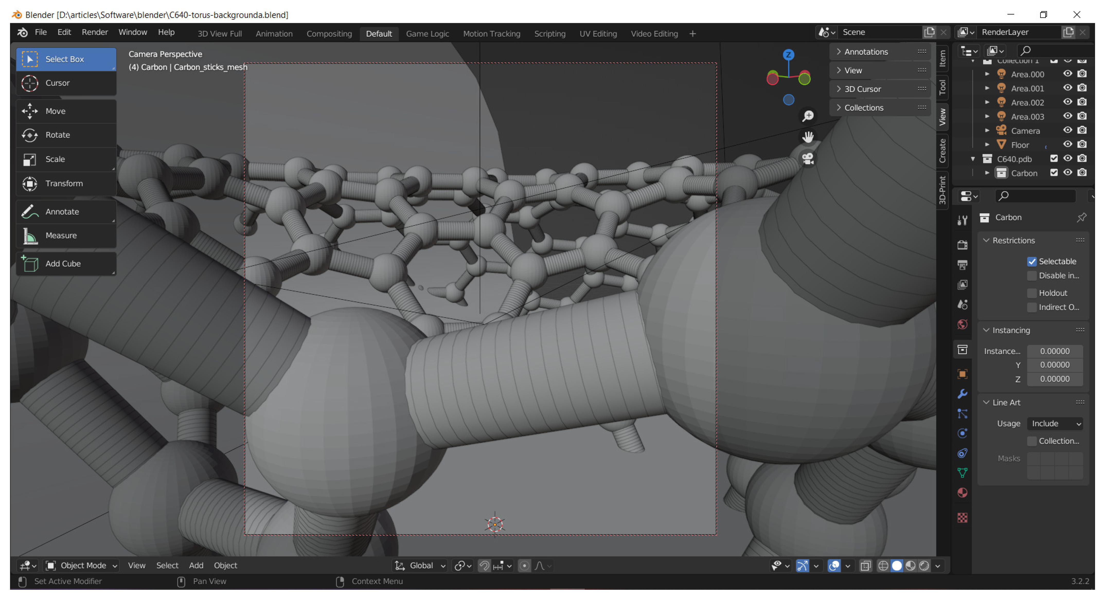
Various computational chemistry software can be used to produce the nanostructures and save the atoms’ coordinates in files of type pdb (Protein Date Base) or xyz (Cartesian coordinates). Such files can be imported into CAD codes as Blender [4] allows, together with the add-ons molblend [79] or atomic [80], the conversion of the nanostructures to a macroscopic object by size rescaling and automatic meshing of the edges of the fullerene- or tube-like objects (see Figure 14). Blender is a free program, oriented towards 3D design, rendering, meshing, sculpting and artistic modeling. It is able to perform some simulations and animations, considering various forces.

In FEM, the deformation of each finite element of the discretized beams determines stress within the grid [81,82]. By its scripting capabilities, Blender can be involved in FEM, but for more advanced simulations, the Blender data can be exported to more specialized software. Thus, the code Blender can be used to create 3D objects and meshes and then export them as .iges or .stp files to Salome-Mecha [83], which is a platform for numerical simulation and has more advanced FEM capabilities. Blender meshes can be exported to Rhino 3D [6] in a variety of formats, as .ply (stanford), .stl, .fbx or .obj (wavefront). Alternatively, an add-on [84] developed for Blender can be used for such conversions. The meshes can be exported to slicer applications such as Cura [85], which can prepare the 3D models for printing with a 3D printer. The UV Blender function can be used for mapping the 3D coordinates into 2D coordinates and unwrapping the 3D objects into planar objects.

4. Conclusions

In the present paper, we attempt to connect two distinct human activity fields, nanochemistry and architecture, which have different aims and address different space and time scales, but they approach similar lattice systems with 2D topologies. The topologies of the carbon-based nanosystems are characterized by nodes that are three-coordinated and lower compared with those of the shell structures. Thus, the nanostructures are characterized by a lower density of edges per node, which means fewer complex grids to cover the same curved surface.

The various mathematical tools developed in the framework of the graph theory and the computing geometry for the description of carbon-type nanosystems and their stability characterization are presented, which might be of use for the design of free-shaped structures in architecture and construction engineering. The enumeration and building methods for the various nanostructures and their use for the design of the shell structures are presented. A particle-based simulation method is proposed for the investigation of the shell systems by the modification of the Elastic Network Model. The simulation method can be applied for the determination of the equilibrium configuration and the dynamics of the shell structures under the influence of external factors such as wind, rain or earthquakes. Thus, the possible scenarios for the shell structures collapsing can be investigated.

Various software products used in computing chemistry, computer graphics, and computer-aided design as well as the conversion data between such software are discussed. Thus, a framework for software from the fields of nanochemistry, architecture, and construction is established, which opens up the opportunity for knowledge transfer from nanochemistry to architecture and construction.