Generation of Synthetic Data for the Analysis of the Physical Stability of Tailing Dams through Artificial Intelligence

Abstract

In this research, we address the problem of evaluating physical stability (PS) to close tailings dams (TD) from medium-sized Chilean mining using artificial intelligence (AI) algorithms. The PS can be analyzed through the study of critical variables of the TD that allow estimating different potential failure mechanisms (PFM): seismic liquefaction, slope instability, static liquefaction, overtopping, and piping, which may occur in this type of tailings storage facilities in a seismically active country such as Chile. Thus, this article proposes the use of four machine learning algorithms, namely random forest (RF), support vector machine (SVM), artificial neural networks (ANN), and extreme gradient boosting (XGBoost), to estimate five possible PFM. In addition, due to the scarcity of data to train the algorithms, the use of generative adversarial networks (GAN) is proposed to create synthetic data and increase the database used. Therefore, the novelty of this article consists in estimating the PFM for TD and generating synthetic data through the GAN. The results show that, when using the GAN, the result obtained by the ML models increases the F1-score metric by 30 percentage points, obtaining results of 97.4%, 96.3%, 96.7%, and 97.3% for RF, SVM, ANN, and XGBoost, respectively.

1. Introduction

The storage of large volumes of data, the latest advances in algorithms, and an increase in computer processing have led artificial intelligence (AI) to position itself within organizations and institutions as a useful tool that allows greater efficiency and productivity in the processes. Mining has not been immune to this evolution and has been gradually incorporating AI into its operation. Identifying exploration zones [1,2], mineral analysis [3,4,5], predicting dangerous environments [6], and predictive maintenance [7] have been some of the advances in this area.

Chile is a mining country and one of the main copper producers in the world, which is why in this research we will focus on analyzing AI algorithms that allow the evaluation of physical stability (PS) in tailings dams (TD) to generate the progressive and safe closure of this type of mining remnants. Tailings are a finely ground solid resulting from ore-extraction processes in mining operations, which must be stored in deposits in a safe and environmentally responsible manner [8]. We aim to use AI algorithms to improve mining processes by analyzing physical stability in tailings deposits.

According to the latest registry of the National Geology and Mining Service (SERNAGEOMIN), there are 757 TD from mining deposits in Chile. Of these, 80% corresponds to the sand tailings dams type (STD), which will be addressed in this paper. The rest corresponds to facilities constructed using borrow materials or thickened tailings deposits (e.g.: filtered tailings deposits, thickened tailings deposits, paste tailings deposits, and in-pit tailings deposits [9]).

Between 1901 and 2013, 38 cases of failures in STD were reported, causing the release of impounded tailings with catastrophic consequences for human lives and environmental damage [10]. Consequently, the mechanisms that generated these faults have been discussed, with conclusions that they would have been produced by a series of complex geotechnical phenomena that occur simultaneously—but not spontaneously—added to the high seismic activity that this zone presents. Therefore, its detection in the early stages would allow corrective measures to be taken to ensure its PS, that is, ensure that the STD does not crumble or overflow when containing the deposited solids. This is where the AI can help us using the various deep learning algorithms, which can be used to detect objects or make predictions of useful signals to analyze PS. Historically, PS monitoring has been reactive, responding to a problem in the structure after an unexpected event, such as an earthquake, or after detecting a particular fault. To reverse this situation, the authorities in charge of safety in the mining field have established regulations to ensure PS regularly in all stages of the life cycle [11,12,13,14].

The periodic evaluation of PS in STD, with a view to closing, implies estimating different potential failure mechanisms (PFM). According to the “Methodological Guide for the Evaluation of the Physical Stability of the Remaining Mining Facilities” [15], the occurrences and PFM are classified as seismic liquefaction, slope instability, static liquefaction, overtopping, and piping. Following the procedures in this guide, it is possible to generate and manage information from geotechnical studies, operational control, and monitoring carried out in TD, including STDs.

The data collected from different deposits raises a relevant question for the mining operation and the safe closure of the facility: Is it possible to estimate the possible PFM? Therefore, this article aims to analyze and study machine learning (ML) algorithms that allow estimating failure potentials. In addition, it will be analyzed whether the data collected from the TD are sufficient or not to build robust models. For the PFM estimation tasks, four state-of-the-art algorithms were selected, namely RF [16], SVM [17], ANN [18], and XGBoost [19], which were chosen for their excellent performance in other applications and investigations [20]. The algorithms identified the five PFM in the STDs, and three classification instances were used (high, significant, or low). Thus, the system analyzed critical variables (input data) and obtained as output a failure potential and its condition (e.g., high overtopping).

One point to keep in mind is that a significant volume of data is needed for the algorithms to correctly generalize and correctly identify potential flaws. However, our research has limited information on TD with its respective characteristics, which is insufficient to generate robust models. For this reason, data generation strategies were used; specifically, the algorithm generative adversarial networks (GAN) [21] will be used to increase the number of samples of the models by generating synthetic data. As a result, failure potential estimation methods were expected to improve their performance when using synthetic data.

The novelty of the article can be seen in two ways. The first of them consists of the determination of the PFM and the PS of the STD for the closure of medium mining. Our proposal consists of using several state-of-the-art algorithms to estimate possible failures. We sought to evaluate PS in DT in a comprehensive manner, unlike the available studies [22,23,24,25,26,27,28,29,30], where PFM are analyzed in isolation. On the other hand, the article proposes the use of GAN to create synthetic data for mining given the problem of insufficient data that occurs in this class of repositories. As far as our knowledge is concerned, there are no data generation works for mining applications associated with tailings deposits.

2. Related Works

This section presents the main advances available in the literature regarding AI for PS and data generation using GAN.

2.1. Artificial Intelligence for Physical Stability

To ensure PS during the life cycle of STD, geotechnical and geometric variables need to be studied and monitored comprehensively to identify possible deviations from the parameters with which they were designed [15]. Currently, solutions have been implemented that allow the evaluation of variables of PS through visual inspections or sensor monitoring; the use of AI for these purposes is little explored. Research in this matter follows two lines; the first refers to estimates and predictions of critical variables that, together with others, could define PS. The other line addresses failure mechanisms such as seismic liquefaction, slope instability, static liquefaction, overtopping, and piping.

Next, we will describe research that seeks to estimate failure mechanisms and critical parameters that define PS using convolutional neural networks, genetic algorithms, artificial neural networks, and long–short-term memory, among others.

Studies carried out in Nevada, the United States, used convolutional neural networks (CNN) to process images and data obtained from unmanned aerial vehicles (UAV) to detect and analyze PFM such as erosion, overtopping, and slope instability [22]. In [23], the C4.5 decision tree model was tested to predict the seismic liquefaction potential of soil based on penetration test data, obtaining classification success rates of 98%. In this same line, studies have been carried out to predict slope stability using ANN with different approaches. One of these was through the combined model of ANN and fuzzy sets [24], where the results showed a better prediction of the failure potential compared to the results of the analytical model. In [25], ANN plus a reliability model was used (first- and second-order reliability method and the Monte Carlo simulation method [26]) to predict the probability of failure, obtaining successful results for the estimation. In [27], the application of two different ANN models to classify slope as stable or unstable and predict its safety factor were discussed. The ANN models were trained using the Bayesian regularization (BRNN), the differential evolution algorithm (DENN), and the Levenberg–Marquardt (LMNN), concluding that the DENN model obtains better results. In [28], a Bayesian network was used for evaluating slope stability using multiple monitoring sources considering that the assessment became more reliable to the extent that specific soil information sources were considered.

Regarding investigations that estimate or predict variables, in [29], image processing was used to analyze the parameter “length of the dry beach” of a TD. CNN was applied to images obtained from monitoring cameras, managing to estimate the parameter with a low error (0.116%) and improving the security conditions of the deposits. In another study, researchers from The Shandong University of Technology, China [30], proposed a predictive model for analyzing the water table in TD. Specifically, they used a genetic algorithm to optimize a back propagation neural network to predict the saturation line of the TD, improving its tendency to change, reducing the risk of failure, and improving its PS condition. Based on historical data from Fuzhou University and Longyan University, China [31], this study analyzed the prediction of the saturation line height of TD. They used the long–short-term memory (LSTM) algorithm and compared it with other classic models such as MLP, SVM, and RNN. The results show that the proposed methodology significantly exceeds traditional methods. In [32], a prediction of geotechnical parameters of soils, such as in situ dry density, compression index, cohesion, and friction angle, was made using machine learning techniques (ML) such as linear regression (LR) analysis, artificial neural network (ANN), support vector machine (SVM), random forest (RF), and M5 tree (M5P). Similarly, in [33], an alternative method was presented to estimate the moisture content (w%) in thickened tailings dams (TTD). This method used ML algorithms based on ANN, SVM, and RF, obtaining accuracy rates between 94% and 97%, generating a benefit in continuous data monitoring operations, and guaranteeing an improvement in physical stability in static and dynamic conditions.

2.2. Data Generation Using GAN

Data generation is increasingly used by developers of deep learning models [34]. It consists of applying algorithms that, from an original data set, generate new data that preserve the characteristics of the original group. These new data are called synthetic data [35].

There are different techniques for generating new data; among the most prominent, we find variational autoencoders (VAEs) [36], denoising diffusion probabilistic models (DDPM) [37], and generative adversarial networks (GAN) [21]. In this work, we used GAN due to its ease of use.

GANs have been used in various investigations and applications due to their excellent generation results. Among GAN’s main uses, we find the generation of images [38], but it has also been used to generate other types of data, such as text [39], time series [40], and generation of works of art [41], among others.

Given the input data’s characteristics for the PS evaluation, we used the GAN to generate tabular data in this research. Within this category, we highlight some algorithms that have been shown to outperform the results obtained by classical methods for generating tabular data, such as CTGAN [42] and TGAN [43]. In addition to these methods, there are some variations, such as CTAB-GAN [44], which are used for complex data distributions. TableGAN [45] incorporates a module to avoid leaking original information. CTGAN [42] uses a conditional generator for the creation of new data, and CopulaGAN [46] is based on a CTGAN but uses the distribution function (CDF) to facilitate data generation.

3. Methodology

The methodology used is experimental, specifically by estimating the PS in STD using AI algorithms. Given the nature of these algorithms in terms of the massive need for data, it is necessary to use alternative mechanisms that know how to complement the available data, in this case, through the GAN model. To carry out these experiments, only data from the deposits corresponding to STD were selected because they concentrate the highest percentage (75.2%) of the deposits of medium-sized mining [9].

3.1. Database

The database has information on the critical variables that allow the PS to be analyzed and is made up of vectors of size 1 × 17 and 17 characteristics that correspond to the values of the critical variables that define PS in STD to generate a progressive and safe closure of this mining facility, according to the SERNAGEOMIN “Methodological Guide for the Evaluation of the Physical of the Remaining Mining Facilities” [15] (please review

Table 1. Critical variables that define PS in STD. Modified from [15].

Category of the Variable	Critical Variable	Datatype
Tailings dams	Typology	Categorical
	Construction method	Categorical
Geometric configuration of the retaining dike of the tailings dam	Freeboard height (m)	Float
	Crest width (m)	Float
	Downstream slope (V:H)	Float
Quality of the sand tailings and compaction level reached for the construction of the retaining dike	Compaction-level standard proctor (SP) or modified proctor (MP) (%)	Int
	Fines content (≤75 µm)	Int
Soil foundation of retaining dike	Foundation soil characterization	Categorical
Instrumentation and monitoring background	Analysis of the piezometric levels in retaining dike	Categorical
	Operation analysis of the drainage system	Categorical
	Accelerometer analysis	Categorical
	Inclinometer analysis	Categorical
	Other analysis in retaining dike: Piezometric levels in soil foundation, distance from de pond to the embankment (upstream slope), vertical deformations, and horizontal and pore pressures	Categorical
Mechanical behavior of the STD (observed during the operational stage of the STD)	Mechanical behavior of the STD	Categorical
Estimation of peak ground acceleration (PGA) for the closure condition	Seismic risk assessments	Categorical
Estimation of floods for the closure condition	Flood risk assessment	Categorical
Degree of implementation of measures to ensure PF in the closure stage	Construction of works and actions	Categorical

for more details). These critical variables were obtained from different sources of information on mining operations, such as closure plans, design projects, resolutions issued by SERNAGEOMIN, operations manuals, official form E-700 for the periodic operational control of TD by SERNAGEOMIN, technical reports prepared by the registry engineer or consultant, and technical reports in response to official letters issued by SERNAGEOMIN. For this work, a database of 57 × 17 critical variables was obtained, and these were obtained after analyzing different sources of information from 57 STD.

With the database, algorithms can be trained to estimate the level of risk for each of the STD in five types of possible faults: seismic liquefaction, slope instability, static liquefaction, overtopping, and piping. Therefore, it was necessary to generate labels for the training of the models. An expert in geotechnics cataloged the data in the database, indicating the failure potentials and their level of risk.

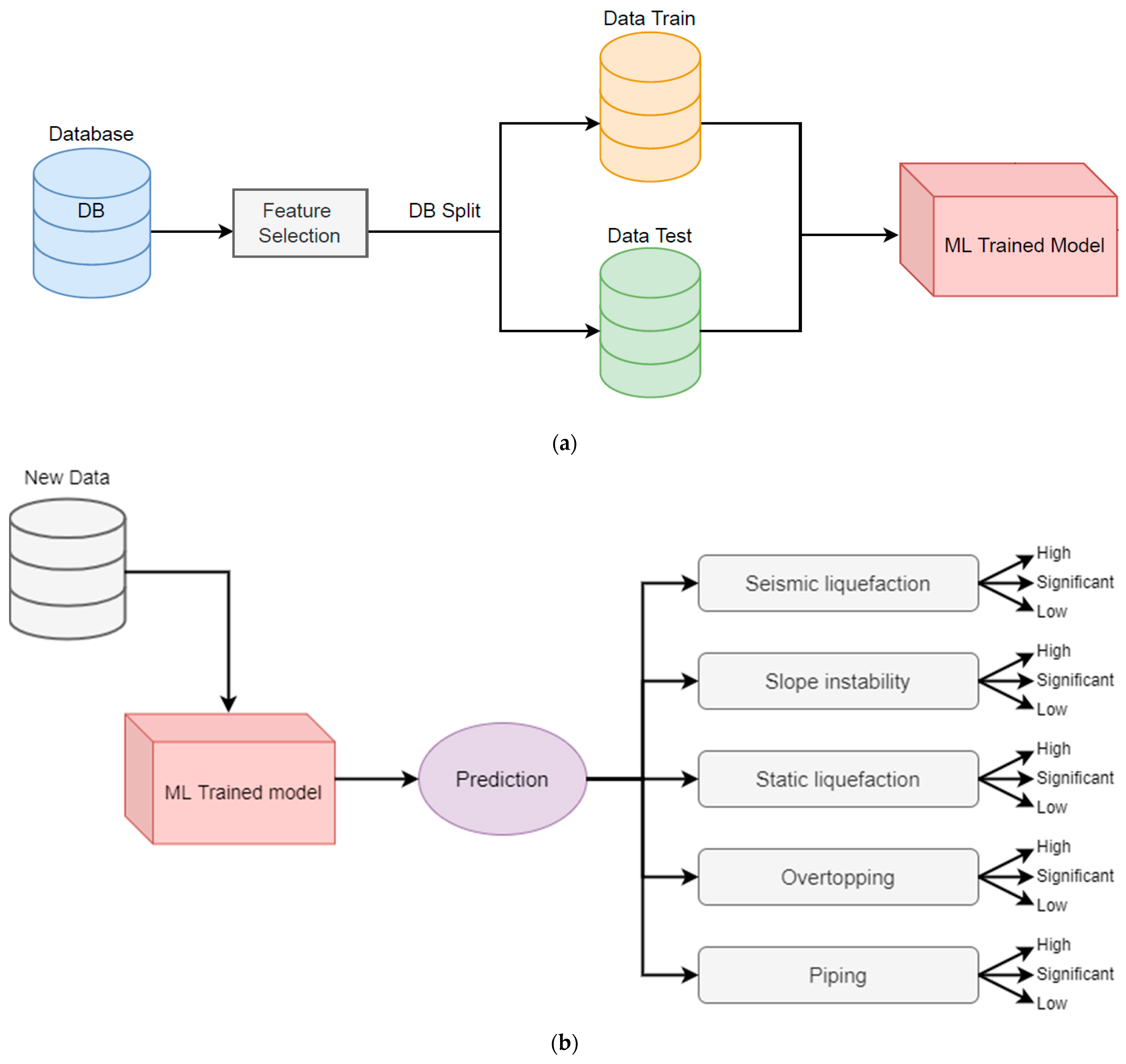
Once the database with its respective labels was created, supervised models were applied to analyze the PS of STD from medium-sized Chilean mining. For this, four models were used, namely RF, SVM, ANN, and XGBoost, according to the scheme shown in Figure 1a. Once the ML algorithms were trained, predictions were made against input data not seen by the models; in this way, the inference of the model was carried out, as shown in Figure 1b. Note that to perform the training and validation of the models, 80% of the total data was used, while 20% was used for the test sets.

Due to the administrative difficulties involved and technical uncertainties in collecting information and due to the lack of a centralized repository with STD data, there was not enough input for model training. To solve this problem, it was proposed to apply data augmentation techniques using GAN [21].

3.2. Machine Learning Algorithms

The following section describes the ML algorithms used in this article. The algorithms were selected due to their excellent generalization capacity and performance against this type of data for prediction tasks.

3.2.1. Random Forest

Random forest is a machine learning algorithm consisting of combined decision trees. A decision tree is a supervised learning technique that, as its name implies, is based on a series of rules organized in the form of a tree to solve classification or regression problems. The intermediate nodes of a decision tree, the branches, represent the solutions, and the final nodes, the leaves, represent the sought predictions. To solve our problem, each decision tree was trained on a random sample of the training data. With this, an improvement in generalization can be obtained when solving the problem [16].

3.2.2. Support Vector Machine

Support vector machine is a supervised learning algorithm used for regression or classification problems. It is based on the search for a hyperplane that optimally separates a data set into two classes by searching for support vectors. For this, various hyperplanes are generated until the one with the maximum distance between the data of each class is found [17]. It is a simple and robust algorithm widely used in machine learning. In this investigation, the algorithm must infer more than two classes; therefore, a multiclass classifier was developed whose outputs correspond to each of the failure occurrence potentials.

3.2.3. Artificial Neural Networks

Artificial neural networks represent a class of models belonging to deep learning (a subfield of ML) inspired by the behavior of human neurons. It allows systems to learn different tasks, such as data prediction and classification, object detection, and natural language processing. ANNs use a backpropagation algorithm to adjust the synaptic weights of the network and thus generate learning. The algorithm obtains the loss (error) in the output, which is propagated to the network. In this way, the synaptic weights are updated to minimize the resulting error for each neuron [18]. In our case, the inputs are given by parameters that define the PS. The network must find and learn specific patterns to infer the different failure occurrence potentials.

3.2.4. XGBoost

Extreme gradient boosting is a widely used machine learning method due to its high effectiveness and accuracy. It corresponds to an open-source software library that uses gradient-powered decision tree (GBDT) in regression and classification problems. A GDBT works in a similar way to a random forest, combining multiple machine learning algorithms to obtain a better model. The difference is that in XGBoost, the trees are built in parallel unlike in GBDT, which are built sequentially.

The term gradient boosting implies the enhancement of a weak model by combining it with several weak models to collectively generate a robust model. The increase of the gradient seeks to minimize the errors with respect to the prediction. The algorithm seeks to boost model performance with high computational speed 10 times faster than existing solutions [19].

3.3. Generative Adversarial Networks (GAN)

GANs are a method for generating synthetic data from an existing data set. They are known for their use in image generation but can also be used for other tasks such as tabular data generation. These networks seek to analyze and learn the distribution of existing data to create new samples to improve the predictions of artificial intelligence models.

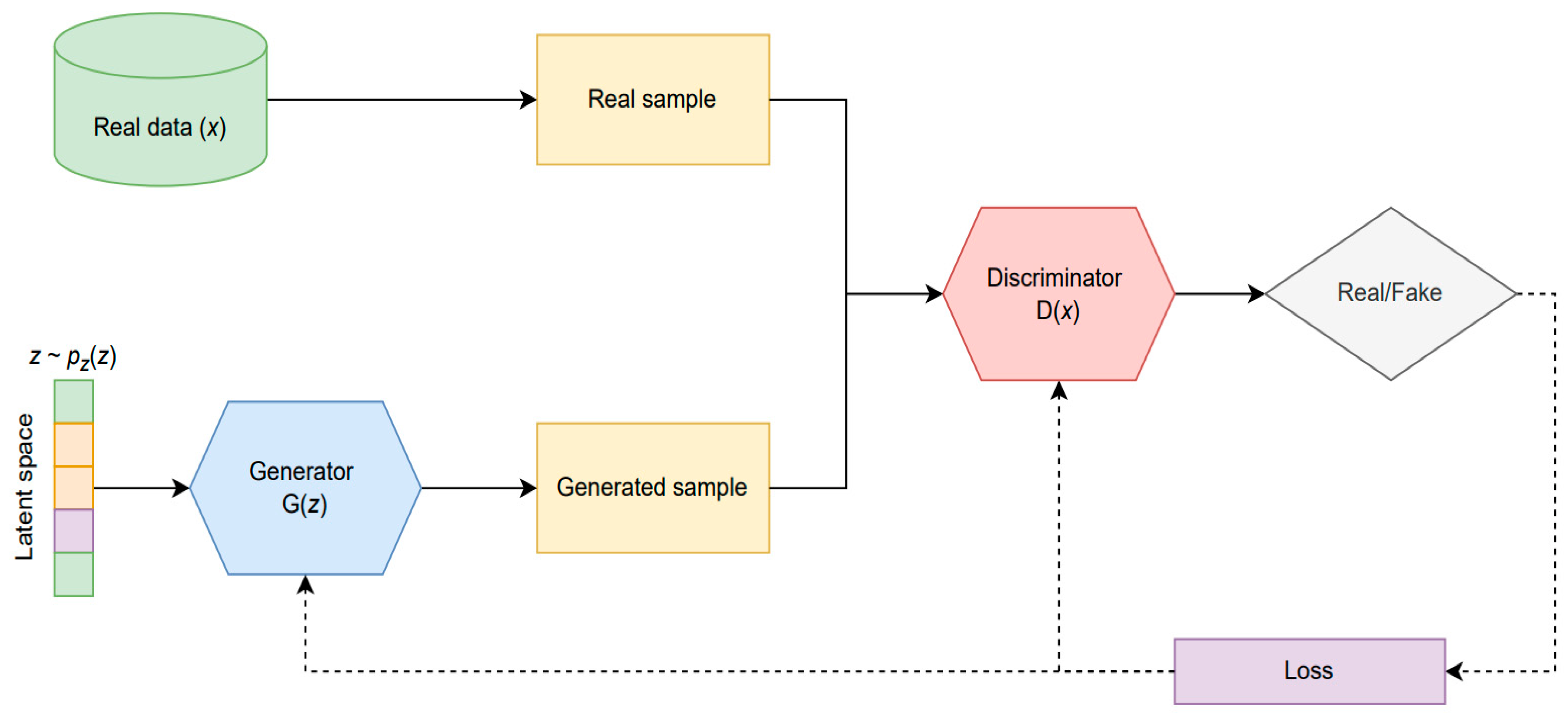
GANs are made up of two deep networks: a generator network (G) that creates data from random noise $p_z(z$) and another discriminator network (D) that analyzes if the data that are entered into the network are real or false. These networks compete in the “min-max game”, aiming to maximize the probability that D correctly labels the generated data and where G minimizes the data generation error so that they are classified as real data by the discriminator. Equation (1) represents the “min-max game” [21].

This min-max game is performed iteratively, alternating between k optimization steps of the network D and one optimization step of G. This seeks to ensure that D does not deviate from the expected optimal values with a sufficiently slow change in G.

In Equation (1), it is possible that G does not have a sufficient gradient to obtain optimal results, and for this reason, initially G is not very precise, and D manages to reject the generated samples with a high percentage of confidence. In this case, log(1 − D(G(z))) saturates. For this reason, Goodfellow [21] proposed to train G by maximizing log(D(G(z))) instead of minimizing log(1 − D(G(z))), optimizing the same value but with a different strategy; this means that both play the same game (min-max game) but in a different way (see pseudocode in [21]).

In conclusion, the training of a GAN has two objectives:

• Maximize the probability that D correctly labels the data as real or synthetic;
• Generator G can generate synthetic data such as the delivered samples so that they are classified as authentic by the discriminator. GAN training ends when the discriminator assigns the probability value to the data equal to 0.5 (D(x) = 0.5) or if it exceeds the number of steps established by the model.

$$mi{n}_{G}ma{x}_{D}V\left(D,G\right)=E_{x~p_{data}\left(x\right)}\left[logD\left(x\right)\right]+E_{z~p_z\left(z\right)}\left[log\left(1-D\left(G\left(z\right)\right)\right)\right]$$

(1)

Figure 2 represents the operation of the GANs. A random noise enters the generating network and generates false data, while the discriminating network tries to discriminate if the generated data are real or false. The generating network will try to create better and better samples (minimizing the value), and the discriminator will try to distinguish them (maximizing). Through error feedback (cost function), the discriminator will be able to identify them better and better, and the generator will learn to produce better and better data. The training of this network concludes when the probability value that the discriminator assigns to the data is equal to 0.5; this means that it is completely deceived by the generator, inferring that the generated data have distributions like that of the actual data. In this work, TGAN [43] was used to generate data.

3.4. Evaluation Metrics

Choosing the correct metrics can be as crucial as adequately selecting the type of models to use. For this reason, this choice may not be so simple, but it indeed turns out to be a valuable tool to distinguish why a model does not obtain the expected results and thus look for alternatives for its improvement.

3.4.1. Machine Learning Evaluation Metrics

To evaluate the algorithms, i.e., RF, SVM, ANN, and XGBoost, we used the accuracy (Equation (2)) and F1-score (Equation (3)) metrics [47]. The first is a measure that considers the number of correct predictions over the total, while the second combines the precision (Equation (4)) and recall (Equation (5)) measures [47], which are ideal for unbalanced data, as in the case of those used for this study. Precision indicates how many of the predicted cases were true positives, while recall shows the number of true-positive cases that the model could predict correctly.

$$Accuracy=\frac{Number of correct predictions}{Total number of predictions}$$

(2)

$$Precision=\frac{TP}{TP+FP}$$

(3)

$$Recall=\frac{TP}{TP+FN}$$

(4)

$$F1 Score=2\times \frac{Precision\times Recall}{Precision+Recall}$$

(5)

where TP—true positive; TN—true negative; FP—false positive; FN—false negative.

3.4.2. GAN Evaluation Metrics

To evaluate the data generated by GAN, we can use different metrics, namely visual or statistical, based on machine learning [48]. Given the nature of the data in this research, we used the first two.

As the name implies, visual metrics consist of a graphical representation of the original and synthetic data. It seeks to verify the results and similarities between both data sets. In this investigation, we used distribution plots to compare the probability density of each critical variable.

In addition to the above, we used a statistical model to compare both sets of data, specifically through a hypothesis test. This test consists of a statistical comparison where a data set is evaluated through a random sample to determine if the hypothesis formulated about the sample should be rejected or not. For this, it was proposed to use the Kolmogorov-Smirnov test (KS test) [49], and we attempted to prove or reject the null hypothesis.

4. Experiments

For the present investigation, three experiments were carried out with the purpose of predicting PS in tailings dam-type deposits. The first experiment consists of using the original database and performing data augmentation using interpolation to fill in missing data. This is done through interpolation techniques based on physically possible values for critical variables of the continuous type using bibliographic data [50,51,52,53,54] such as closure plans, design projects, resolutions issued by SERNAGEOMIN, operations manuals, officials form E-700, technical reports prepared by the registry engineer or consultant, and technical reports in response to official letters issued by SERNAGEOMIN (see

Table 2. Physically possible values for continuous geometrics and geotechnical control critical variables that define PS in STD from medium-sized Chilean mining. According to [15].

Category of the Variable	Critical Variable	Physically Possible Value
Geometric configuration of the retaining dike of the tailings dam	Freeboard height (m)	0.5–5
	Crest width (m)	0.5–7
	Downstream slope (V:H)	1:2–1:4
Quality of the sand tailings and compaction level reached for the construction of the retaining dike	Compaction-level standard Proctor (SP) or modified Proctor (MP) (%)	90–100
	Fines content (≤75 µm)	0–30

).

The GAN is then applied to create 100 totally new synthetic data. The second experiment consists of using the training data from experiment 1, but now, a class balance is performed, and then, the GAN is used to create 100 synthetic data with balanced classes. The third experiment is identical to experiment 2, but now, 1000 synthetic data are generated. The idea is to analyze if the performance and success rates of the ML models increase when using the generated synthetic data.

Once the synthetic data were created with the GAN, new experiments were performed to determine the PFM using four supervised ML algorithms, RF, SVM, ANN, and XGBoost. The results obtained were analyzed using the F1-score and accuracy metrics. Regarding the hyperparameters, in the case of RF, the metrics were evaluated by varying the number of decision trees that make up the model, using the values 10, 100, 1000, and 10,000. In the case of SVM, the tests were performed by varying the regularization parameter (C), which penalizes the errors associated with the classes that may be in the classification margin; the lower the value of parameter C, the fewer errors are penalized. Tests were performed for values of C equal to 1, 10, 100, and 1000. In addition to this adjustment, tests were performed by varying the different kernel types (linear, poly, RBF, sigmoid). For the ANN case, we used a categorical cross-entropy loss function and the ADAM optimizer to perform backpropagation learning. Tests were performed varying hyperparameters, setting the parameters to 500 epochs with a batch size of 50, with 10 hidden layers with RELU activation with Sigmoid in the output layer. For the case of XGBoost, we selected Gbtree among the different boosters to use since it occupies tree-based models, which is more convenient than Gblinear for this type of task as well as faster than Dart booster. As a learning objective, a regression with squared loss was specified, and tests were performed varying the learning rate and the number of branch nodes, configuring the parameters at a learning rate of 0.3 and 6 branch nodes to avoid overfitting of the model.

To analyze the performance of the ML models, the results of the three experiments carried out in the generation of synthetic data obtained with TGAN were used. Thus, the first experiment using ML models consists of classifying the 100 unbalanced synthetic data. The second experiment seeks to classify the data obtained from the second experiment with TGAN, that is, 100 balanced synthetic data. The third experiment tries to classify the 1000 synthetic data obtained with TGAN.

5. Experiment Results

The results obtained from the experiments carried out for the generation of data with TGAN and the classification of the potential failure mechanisms with the ML algorithms are presented below.

5.1. GAN Experiment Results

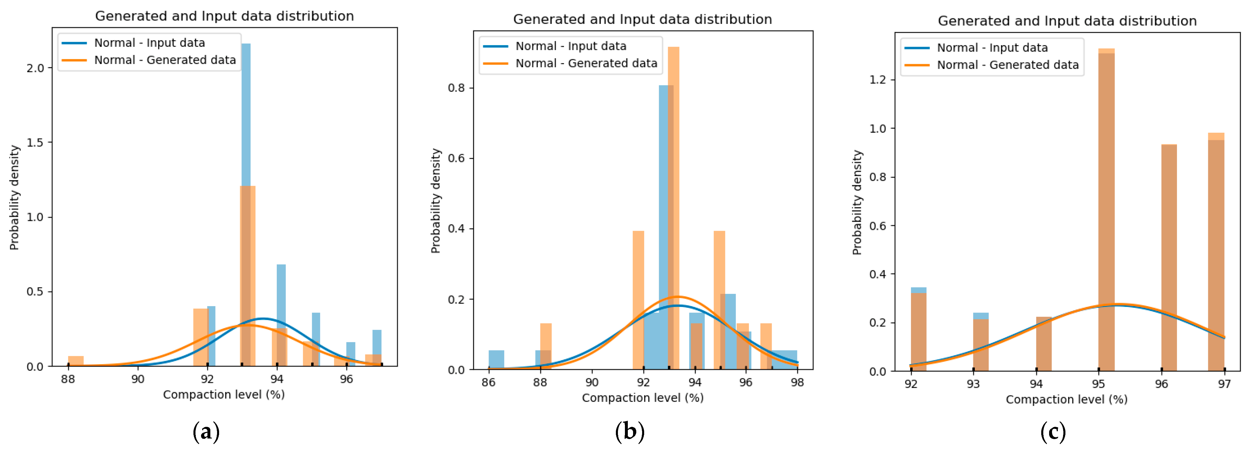
To evaluate the results of the three TGAN experiments, a visual evaluation and a statistical hypothesis were used. Regarding the visual evaluation, the distribution of real data and generated data was compared. An example is presented in Figure 3 for the “compaction-level” feature. As the synthetic data increases, the distributions of the real and synthetic data adjust more and more, demonstrating an adequate generation with the TGAN model.

In addition, an evaluation was carried out using a statistical metric, specifically applying the KS hypothesis test for two distributions. Two hypotheses were proposed: the null hypothesis and the alternative. The null hypothesis corresponds to the fact that both distributions are equal, while the alternative posits a difference between them.

Table 3. Application of KS Test for geometrics and geotechnical control critical variables.

Critical Variable	Statistic	p-Value
Freeboard height (m)	0.02185	0.97301
Crest width (m)	0.02384	0.94349
Compaction level (%)	0.00905	0.99999
Fines content (≤75 µm)	0.00921	0.99999

shows the results of the application of this test for four continuous critical variables: freeboard height, crest width, compaction level, and fines content. It is possible to observe for the total of the variables statistic values close to zero and high values of p-value; this is enough evidence to sustain that under a confidence level of 95%, both distributions are statistically equal, for which the hypothesis would be accepted: null hypothesis [49].

5.2. ML Algorithms Experiment Results

The results obtained from the application of the ML models to the synthetic data obtained with TGAN are presented below. The results are presented in

Table 4. Summary of results obtained in the RF, SVM, ANN, and XGBoost models PFM to be considered for the evaluation of PS of STD in the closure phase. Bold values show the best results.

PFM	Experiment	F1-Score				Accuracy
		RF	SVM	ANN	XGBoost	RF	SVM	ANN	XGBoost
Seismic liquefaction	1	66.7%	62.7%	66.7%	66.7%	100%	95.0%	100%	100%
	2	83.3%	83.3%	77.0%	100%	100%	85.0%	80.0%	100%
	3	99.5%	99.5%	99.3%	100%	99.5%	99.5%	99.5%	100%
Slope instabilities	1	66.7%	66.7%	66.7%	66.7%	100%	100%	100%	100%
	2	95.0%	89.3%	79.7%	86.3%	95.0%	90.0%	85.0%	80.0%
	3	95.5%	92.5%	95.0%	95.7%	95.5%	92.5%	95.0%	95.5%
Static liquefaction	1	66.7%	63.3%	66.7%	66.7%	100%	95.0%	100%	100%
	2	100%	85.0%	78.3%	100%	100%	85.0%	80.0%	100%
	3	100%	99.5%	99.3%	100%	100%	99.5%	99.5%	100%
Overtopping	1	66.7%	66.7%	66.7%	66.7%	100%	100%	100%	100%
	2	100%	65.7%	57.3%	55.3%	80.0%	75.0%	75.0%	55.0%
	3	92.5%	90.5%	89.7%	91.0%	92.5%	90.5%	91.0%	89.5%
Piping	1	66.7%	66.7%	66.7%	66.7%	100%	100%	100%	100%
	2	100%	83.3%	70.3%	100%	100%	85.0%	75.0%	100%
	3	99.3%	99.3%	100%	100%	99.5%	99.5%	100%	100%
Mean	1	66.7%	65.2%	66.7%	66.7%	100%	98.0%	100%	100%
	2	95.7%	81.3%	72.5%	88.3%	95.0%	84.0%	79.0%	87.0%
	3	97.4%	96.3%	96.7%	97.3%	97.4%	96.3%	97.0%	97.0%

. The evaluation of the table was carried out by analyzing the metrics F1-score and accuracy of the models. The results are summarized only in a table that shows the metrics of each experiment, and the best results are highlighted in bold for the four models used.

Table 4 summarizes the best results for each algorithm, according to failure mechanism and experiment. In general terms, the best results were obtained in experiment 3 using the RF model, reaching average values of F1-Ssore and accuracy equal to 97.4%, reflecting an increase of 30 percentage points in F1-score with respect to experiment 1. The rest of the models also obtained high metrics when using 1000 balanced synthetic data, which shows that the use of the GAN is relevant to improve the performance of the models. It is important to mention that although the accuracy is very good in some cases, it should always be contrasted with the F1-score metric since having a high accuracy but a low F1-score indicates that the model can classify only one class correctly and not the others. Regarding the classification of potential failure mechanisms, there are some classes that are easier than others to classify by models; seismic liquefaction obtained high success rates with all methods compared to overtopping, for example.

These results demonstrate that as we complement and improve the quality of the input data, the algorithms better predict the occurrence potentials for each failure mechanism concerning the F1-score metric. No significant changes are observed between the different experiments for the accuracy metric.

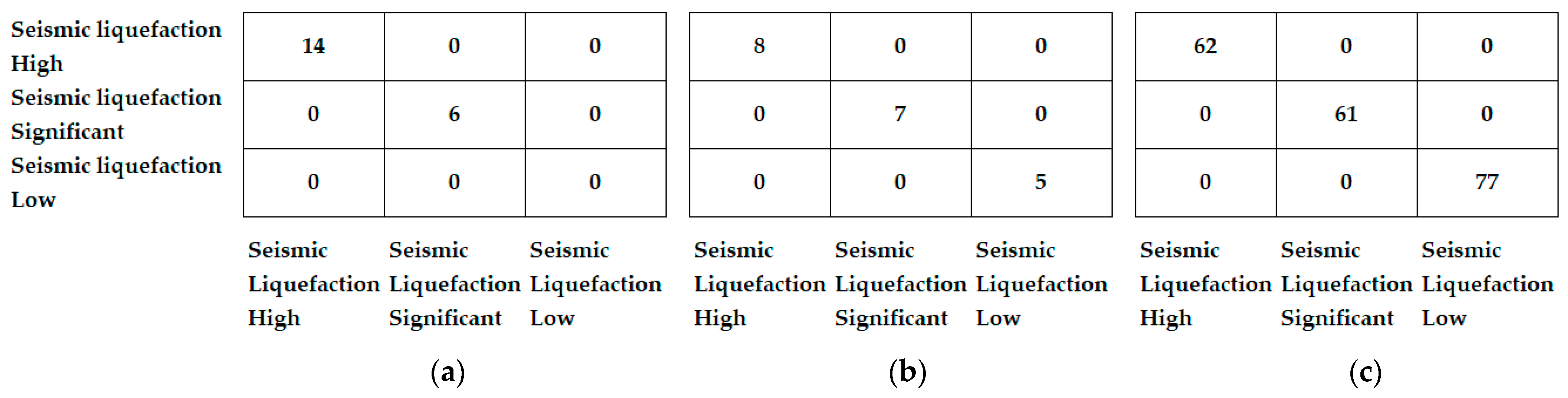
Figure 4 shows the confusion matrix for the prediction of the seismic liquefaction fault mechanism, obtained with the XGBoost model, for each of the experiments. For experiment 1, the model correctly predicts the class “high” and “significant”; however, the data set is very small, so there is no information for the class “low”, obtaining 66.7% in the metric F1-score. As we balance and increase the amount of data using TGAN, we observe an improvement in the confusion matrix, obtaining 100% in the F1-score metric for experiment 2 and 3.

To the best of our knowledge, the generation of synthetic data to make up for the insufficiency of data with the aim of classifying STD failure mechanisms has not been addressed in other works. However, the GAN approach has been applied to a variety of problems in other contexts, ranging from emotion classification [55] to image classification [56].

6. Conclusions and Future Work

This research presents a methodology to evaluate the STD in view of a progressive and safe closure of this remaining mining facility using ML algorithms, which allow a periodic and safe evaluation of geotechnical and geometric variables of the reservoirs in an integral way. Due to the lack of data required for robust training, the application of a tabular data generation model that allows the creation of synthetic data to develop algorithms for classification tasks is also presented.

The experimental results show that it is possible to evaluate the PS of TD through the ML algorithms due to the good results obtained in the F1-score and accuracy metrics for the classification models. However, it is shown that the lack of data is a problem that must be compensated using generative models. The methodology presented in this research corrects this problem by applying GAN to tabular data. When using synthetic data, a significant improvement in the classification results is observed, increasing the performance of the analyzed models. Average percentages of F1-score equal to 97.4% for the RF case, 96.7% for the ANN case, 96.3% for the SVM case, and 97.3% for XGBoost were obtained, increasing the results by around 30 percentage points of classification.

As future work, it will be interesting to carry out tests with other types of TD, such as tailings dams, thickened tailings, filtered tailings, and paste tailings. The difference with what was applied in this research, which considered only STD-type deposits, lies in the critical variables that define PS according to the type of deposits. In case of insufficient samples for model training, the same solution of this research could be implemented through data generation using GAN for tabular data or adding new generation models, as in the case of diffusion models.

References

- Balaniuk, R.; Isupova, O.; Reece, S. Mining and tailings dam detection in satellite imagery using deep learning. arXiv 2020, arXiv:2007.01076v1. [Google Scholar] [CrossRef] [PubMed]
- Keykhay-Hosseinpoor, M.; Kohsary, A.H.; Hossein-Morshedy, A.; Porwal, A. A machine learning-based approach to exploration targeting of porphyry Cu-Au deposits in the Dehsalm district, eastern Iran. Ore Geol. Rev. 2020, 116, 103234. [Google Scholar] [CrossRef]
- Maitre, J.; Bouchard, K.; Bedard, P. Mineral grains recognition using computer vision and machine learning. Comput. Geosci. 2019, 130, 84–93. [Google Scholar] [CrossRef]
- Lorenz, S.; Ghamisi, P.; Kirsch, M.; Jackisch, R.; Rasti, B.; Gloaguen, R. Feature extraction for hyperspectral mineral domain mapping: A test of conventional and innovative methods. Remote Sens. Environ. 2021, 252, 112129. [Google Scholar] [CrossRef]
- Cardoso-Fernandes, J.; Teodoro, A.C.; Lima, A.; Roda-Robles, E. Evaluating the performance of support vector machines (SVMs) and random forest (RF) in Li-pegmatite mapping: Preliminary results. In Earth Resources and Environmental Remote Sensing/GIS Applications X; SPIE: Bellingham, DC, USA, 2019; pp. 146–157. [Google Scholar]
- Zhou, J.; Li, X.; Shi, X. Long-term prediction model of rockburst in underground openings using heuristic algorithms and support vector machines. Saf. Sci. 2012, 50, 629–644. [Google Scholar] [CrossRef]
- Kruczek, P.; Gomolla, N.; Hebda-Sobkowicz, J.; Michalak, A.; Śliwiński, P.; Wodecki, J.; Stefaniak, P.; Agnieszka, W.; Zimroz, R. Predictive maintenance of mining machines using advanced data analysis system based on the cloud technology. In Proceedings of the 27th International Symposium on Mine Planning and Equipment Selection-MPES 2018; Springer: Cham, Switzerland, 2019; pp. 459–470. [Google Scholar]
- SERNAGEOMIN Site. Available online: https://www.sernageomin.cl/ (accessed on 10 March 2022).
- SERNAGEOMIN. Datos Públicos Depósito de Relaves. Catastro de Depósitos de Relaves en Chile 2020. Available online: https://www.sernageomin.cl/datos-publicos-depositode-relaves/ (accessed on 10 March 2022).
- Villavicencio, G.; Palma, J.; Fourie, A.; Valenzuela, P.; Espinace, R. Failures of sand tailings dams in a highly seismic country. Can. Geotech. J. 2014, 51, 454–456. [Google Scholar] [CrossRef]
- Biblioteca del Congreso Nacional de Chile. Decreto Supremo N° 132: Reglamento de Seguridad Minera. Available online: https://www.bcn.cl/leychile/navegar?idNorma=221064 (accessed on 20 May 2022).
- Biblioteca del Congreso Nacional de Chile. Decreto Supremo N° 248: Reglamento para la Aprobación de Proyectos de Diseño, Construcción, Operación y Cierre de los Depósitos de Relave. Available online: https://www.bcn.cl/leychile/navegar?idNorma=259901 (accessed on 20 May 2022).
- Biblioteca del Congreso Nacional de Chile. Ley 20.819: Modifica la Ley N° 20.551: Regula el Cierre de Faenas e Instalaciones Mineras. Available online: https://www.bcn.cl/leychile/navegar?i=1075399&f=2015-03-14 (accessed on 20 May 2022).
- Biblioteca del Congreso Nacional de Chile. Decreto N° 41: Aprueba el Reglamento de la Ley de Cierre de Faenas e Instalaciones Mineras. Available online: https://www.bcn.cl/leychile/navegar?idNorma=1045967&idParte=9314317&idVersion=2020-06-23 (accessed on 20 May 2022).
- SERNAGEOMIN. Guía Metodológica para Evaluación de la Estabilidad Física de Instalaciones Mineras Remanentes. 2018. Available online: https://www.sernageomin.cl/wp-content/uploads/2019/06/GUIA-METODOLOGICA.pdf (accessed on 10 March 2022).
- Breiman, L. Random Forests. Mach. Learn. 2001, 45, 5–32. [Google Scholar] [CrossRef]
- Cortes, C.; Vapnik, V. Support-Vector Networks. Mach. Learn. 1995, 20, 273–297. [Google Scholar] [CrossRef]
- Bishop, C.M. Neural Networks for Pattern Recognition; Oxford University Press: New York, NY, USA, 1995. [Google Scholar]
- Chen, T.; Guestrin, C. XGBoost: A Scalable Tree Boosting System. arXiv 2016, arXiv:1603.0274. [Google Scholar]
- Sarker, I.H. Machine Learning: Algorithms, Real-World Applications and Research Directions. SN Comput. Sci. 2021, 2, 160. [Google Scholar] [CrossRef] [PubMed]
- Goodfellow, I.; Pouget-Abadie, J.; Mirza, M.; Xu, B.; Warde-Farley, D.; Ozair, S.; Courville, A.; Bengio, Y. Generative Adversarial Nets. Adv. Neural Inf. Process. Syst. 2014, 27, 2672–2680. [Google Scholar]
- Nasategaym, F. Detection and Monitoring of Tailings Dam Surface Erosion Using UAV and Machine Learning. Master’s Thesis, University of Nevada, Reno, NV, USA, 2020. [Google Scholar]
- Ardakanivand, A.; Kohestani, V.R. Evaluation of liquefaction potential based on CPT results using C4.5 decision tree. J. AI Data Min. 2015, 3, 85–92. [Google Scholar]
- Ni, S.H.; Lu, P.C.; Juang, C.H. A fuzzy neural network approach to evaluation of slope failure potential. J. Microcomput. Civ. Eng. 1996, 11, 56–66. [Google Scholar] [CrossRef]
- Cho, S.E. Probabilistic stability analyses of slopes using the ANN-based response surface. Comput. Geotech. 2009, 36, 787–797. [Google Scholar] [CrossRef]
- De Rivera, D.P.S. Deducción de distribuciones: El método de Monte Carlo. In Fundamentos de Estadística; Alianza Editorial S.A., Ed.; Alianza Editorial: Madrid, Spain, 2001. [Google Scholar]
- Das, S.; Biswal, R.; Sivakugan, N.; Das, B. Classification of slopes and prediction of factor of safety using differential evolution neural networks. Environ. Earth Sci. 2011, 64, 201–210. [Google Scholar] [CrossRef]
- Peng, M.; Li, X.Y.; Li, D.Q.; Jiang, S.H.; Zhang, L.M. Slope safety evaluation by integrating multi-source monitoring information. Struct. Saf. 2013, 49, 65–74. [Google Scholar] [CrossRef]
- Yang, J.; Yeqing, S.; Li, Q.; Qian, Z. Measure Dry Beach Length of Tailings Pond Using Deep Learning Algorithm. In Proceedings of the 2019 Conference on Robotics, Intelligent and Artificial Intelligence, Shanghai, China, 20–22 September 2019; pp. 503–508. [Google Scholar]
- Tongle, X.; Yingbo, W.; Kang, C. Tailings saturation line prediction based on genetic algorithm and BP neural network. J. Intell. Fuzzy Syst. 2016, 30, 1947–1955. [Google Scholar] [CrossRef]
- Jiahong, F. Research on Tailings Pond Risk Prediction Algorithm Based on Support Vector Machine. Master’s Thesis, Zhejiang University of Technology, Hangzhou, China, 2017. [Google Scholar]
- Puri, N.; Prasad, H.D.; Jain, A. Prediction of geotechnical parameters using machine learning techniques. Procedia Comput. Sci. 2018, 125, 509–517. [Google Scholar] [CrossRef]
- Villavicencio, G.; Piña, O.; Hermosilla, G.; Allende-Cid, H.; Suazo, G.; Araya, V. Estimation of Moisture Content in Thickened Tailings Dams: Machine Learning Techniques Applied to Remote Sensing Images. IEEE Access 2021, 9, 16988–16998. [Google Scholar] [CrossRef]
- Nikolenko, S. Synthetic Data for Deep Learning; Steklov Institute of Mathematics: St. Petersburg, Russia; San Francisco, CA, USA, 26 September 2019. [Google Scholar]
- Rubin, D. Discussion Statistical Disclosure Limitation. J. Off. Stat. 1993, 9, 461–468. [Google Scholar]
- Kingma, D.P.; Welling, M. Auto-encoding variational Bayes. In Proceedings of the Internacional Conference on Learning Representations, Banff, AB, Canada, 14–16 April 2014. [Google Scholar]
- Ho, J.; Jain, A.; Abbeel, P. Denoising Diffusion Probabilistics Models. arXiv 2020, arXiv:2006.11239. [Google Scholar]
- Joo, D.; Kim, D.; Kim, J. Generating a fusion image: One’s identity and Another’s shape. In Proceedings of the IEEE Conference on Computer Vision and Pattern Recognition, Salt Lake City, UT, USA, 18–23 June 2018; pp. 1635–1643. [Google Scholar]
- Nie, W.; Narodytska, N.; Patel, A. Relgan: Relational generative adversarial networks for text generation. In Proceedings of the International Conference on Learning Representations (ICLR), Louisiana, LA, USA, 6–9 May 2019; pp. 1–20. [Google Scholar]
- Smith, K.; Smith, A. Conditional GAN for timeseries generation. arXiv 2020, arXiv:2006.16477v1. [Google Scholar]
- Elgammal, A.; Liu, B.; Elhoseiny, M.; Mazzone, M. CAN: Creative adversarial networks, generating ‘Art’ by learning about styles and deviating from style norms. In Proceedings of the 8th International Conference on Computational Creativity, ICCC, Atlanta, GA, USA, 19–23 June 2017. [Google Scholar]
- Xu, L.; Skoularidou, M.; Infante, A.C.; Veeramachaneni, K. Modeling Tabular Data Using Conditional GAN. In Proceedings of the 33rd International Conference on Neural Information Processing Systems, Vancouver, BC, Canada, 8–14 December 2019; pp. 7335–7345. [Google Scholar]
- Xu, L.; Veeramachaneni, K. Synthesizing Tabular Data using Generative Adversarial Networks. arXiv 2018, arXiv:1811.11264. [Google Scholar]
- Zhao, Z.; Kunar, A.; Van der Scheer, H.; Birke, R.; Chen, L.Y. CTAB-GAN: Effective Table Data Synthesizing. arXiv 2021, arXiv:2102.08369. [Google Scholar]
- Park, N.; Mohammadi, M.; Gorde, K.; Jajodia, S.; Park, H.; Kim, Y. Data synthesis based on generative adversarial networks. arXiv 2018, arXiv:1806.03384. [Google Scholar] [CrossRef]
- CopulaGAN Model. Available online: https://sdv.dev/SDV/user_guides/single_table/copulagan.html (accessed on 8 June 2022).
- Goutte, C.; Gaussier, E. A Probabilistic Interpretation of Precision, Recall and F-Score, with Implication for Evaluation. Lect. Notes Comput. Sci. 2005, 3408, 345–359. [Google Scholar] [CrossRef]
- Bourou, S.; El Saer, A.; Velivassaki, T.H.; Voulkidis, A.; Zahariadis, T. A Review of Tabular Data Synthesis Using GANs on an IDS Dataset. Information 2021, 12, 375. [Google Scholar] [CrossRef]
- Hodges, J.L., Jr. The Significance Probability of the Smirnov Two-Sample Test. Ark. För Mat. 1958, 3, 469–486. [Google Scholar] [CrossRef]
- Barrera, S.; Lara, J. Geotechnical characterization of cycloned sands for the seismic design of tailings deposits. In Proceedings of the 3rd International Congress on Environmental Geotechnics, Lisbon, Portugal, 7–11 September 1998; pp. 201–206. [Google Scholar]
- Barrera, S.; Valenzuela, L.; Campaña, J. Sand tailings dams: Design, construction and operation. In Proceedings of the Tailings and Mine Waste 2011, Vancouver, BC, Canada, 6–9 November 2011. [Google Scholar]
- Verdugo, R. Compactación de Relaves. In Proceedings of IV Congreso Chileno de Ingeniería Geotécnica; Universidad Federico Santa María, Sociedad Chilena de Geotecnia: Valparaíso, Chile, 1997; pp. 29–41. [Google Scholar]
- Villavicencio, G. Méthodologie Pour Evaluer la Stabilité Mécanique des Barrages de Résidus Miniers. Ph.D. Thesis, Civil Engineering Dissertation. University Blaise Pascal, Clermont Ferrand, France, 2009. [Google Scholar]
- Villavicencio, G.; Breul, P.; Bacconnet, C.; Boissier, D.; Espinace, A.R. Estimation of the variability of tailings dams properties in order to perform probabilistic assessment. Geotech. Geol. Eng. 2011, 29, 1073–1084. [Google Scholar] [CrossRef]
- Zhu, X.; Liu, Y.; Li, J.; Wan, T.; Qin, Z. Emotion Classification with Data Augmentation Using Generative Adversarial Networks. arXiv 2017, arXiv:1711.00648. [Google Scholar]
- Hung, S.; Gan, J. Augmentation of Small Training Data Using GANs for Enhancing the Performance of Image Classification. In Proceedings of the 2020 25th International Conference on Pattern Recognition (ICPR), Milan, Italy, 10–15 January 2021; pp. 3350–3356. [Google Scholar] [CrossRef]