Land Plots Evaluation for Agriculture and Green Energy Projects: How to Overcome the Conflict Using Mathematics

Abstract

Seventeen sustainable development goals were formulated to create a harmonious world order for the benefit of different nations and peoples. At the same time, economic practice provides a lot of examples of conflicts of an economic nature between individual sustainable development goals. One of these conflicts is the need for environmental imperatives and economic growth when a massive assessment of land used for crop production and green energy projects is needed. The present paper considers a non-traditional approach to the mass evaluation of land plots on the condition that geographic information systems provide the main source of information, such as the case of land allocation for green energy facilities and evaluation of agricultural plots. The novelty of the proposed approach firstly means the development of a comparative approach, which receives much less attention in the valuation literature than cost and income approaches, as it can give an adequate picture of the current state of the market. The model includes the study of the entire dataset, the selection of model distributions and the construction of estimates based on model distributions. The methodology of multivariate lognormal distribution of factors and prices of analogues is used. The peculiarity of the market evaluation of land plots in such cases is, as a rule, the absence of rank predictors and sufficient number of continuous predictors, which provides a base for the application of a novel approach. The method of express testing of hypotheses about joint normality of logarithms of values of pricing factors and prices is proposed. The market value is estimated as an estimate of the modal value of conditional lognormal price distribution. Secondly, the problem of market valuation is solved in case of the almost complete absence of information about price-forming factors in the areas being assessed, and thirdly, the factors are determined based on geoinformation databases (distance to the nearest large city, regional center, federal highway, large rivers, lakes, and solid waste landfills), which allow for market assessment in the absence of information on pricing factors for land plots, except for the offer price and the plot area. The research was necessitated by the claim to determine on a specific date the cadastral value of agricultural land for the purposes of taxation, corresponding to the market value, in the almost complete absence of information on pricing factors in the assessed areas. The value of land reflects a complex combination of factors, so the use of the proposed mathematical toolkit allows for building a consistent model for the evaluation of land where improvements are absent or have no value in terms of land acquisition purposes.

1. Introduction

The “Transforming our world: the 2030 Agenda for Sustainable Development” [1] strategy sets the goal of an integrated approach to sustainable development. In this regard, cooperation between state and non-state actors and in different sectors of the economy becomes one of the important conditions for achieving the sustainable development goals. This study focuses on two goals, namely (goal 2) putting an end to hunger and ensuring food security and improved nutrition and promoting sustainable agriculture (1), and (goal 7) ensuring universal access to affordable, reliable, sustainable, and modern energy for all (2) [2].

The diversity of economic activities, in which state and non-state actors are involved, is ensured by the use of various instruments, the action of which often leads to a conflict of their interests, and as a consequence, to real economic conflicts. In particular, this applies to land plots—a finite resource in real economic systems. Just as any finite resource, land has its own value and its most objective evaluation is an effective tool for eliminating contradictions in achieving the goals for sustainable development.

Many countries adopted energy strategies aimed at the transition to a low-carbon economy. The paper by Gielen, Miketa, Gorini, and Carvajal [3] contains an analysis of 18 main energy scenarios for the period up to 2050. It should be noted that these strategies aim to increase the share of renewable energy sources (RES) in the primary energy balance from 48 to 94 percent by the end of the period. The share of wind-based renewables in electricity generation could be about 7500 TWh by 2050, a 10-fold increase over 2010 [4]. On average, one 2.5–3 MW wind power generator installed on a piece of land could produce more than 6 million kWh per year, or 0.006 TWh [5]. Non-complicated calculations show that about 1.25 million wind power generators will have to be built and installed in order to generate electricity in the given volumes. Considering that on average one wind power generator with the capacity of 2.5–3 MW takes about 0.8 hectares [6], then the total area of land under the power generators would be about 1 million hectares. As the U.S. experience shows, wind and solar energy production requires at least 10 times more land per unit of energy produced than coal or natural gas-fired power plants, including land used to produce and transport fossil fuels. Therefore, the development of green energy combined with land usage such as agriculture can minimize land usage conflicts according to Gross [7]. The acuteness of this issue is also noted in another study [8], which shows that wind and solar energy systems often require large amounts of land and airspace, so their growing presence is generating a lot of new and complex land usage conflicts. According to Santangeli et al. [9], another problem inherent in bioenergy projects is the serious damage to biodiversity, since half of their global potential is concentrated in areas with the highest levels of biodiversity. According to Fritsche et.al. [10], a tool to solve these problems is land-use planning in coordinating large-scale and decentralized deployment of renewable energy systems. The mathematical apparatus we propose can be used as a tool to solve this class of problems.

In our case, there is an acceptable amount of data, but a specific feature of the assessment of agricultural plots is the extremely scarce information about pricing factors (as a rule, there is no information about engineering support, facilities or buildings on the plots, there are no factors traditionally considered in the assessment of residential or summer cottages, etc.). At the same time, it is obvious that the market value of agricultural facilities is, firstly, lower than the market value of land plots allocated to residential, commercial, and industrial development, and, secondly, it significantly depends on the location and accessibility of the land plot. Ideally, we should have information on soil compositions and other agrophysical parameters, but it is still difficult to access.

The present study fills the research gap as it claims to determine on a specific date the cadastral value of agricultural land for taxation purposes, corresponding to the market value, in the almost complete lack of information on pricing factors in the assessed areas. A further aim of the study is to identify fragments of the territory with a minimum cost of land plots as agricultural plots, so that the optimal location for green energy facility deployment can be determined, because such facilities claim large areas that can only be withdrawn from agricultural land. Accordingly, it is reasonable to carry out such withdrawal from the lands of the lowest value and, therefore, from the value in terms of agricultural production.

The paper is organized so that after the literature review, the Materials and Methods section describes the data used for analysis, including the mathematical and statistical methods used for model development. The proposed novel model is introduced in Section 3 in which the lognormal nature of the model is also verified. Section 4 presents the application of the theoretical model for the Leningrad region. Finally, the Conclusion section summarizes the findings and reasons for the model’s value to achieve specific sustainability goals.

2. Literature Review

With dynamic changes in the information environment, the availability of a wide range of application software prompts many researchers in the field of real estate appraisal to look for new, non-traditional methods of real estate evaluation, based on the processing of large market data. In the tasks related to land allocation for green energy, extensive data on plots—if possible, not built-up—are considered that result in a comparison of the assessment of the market value of the agricultural use of plots with the assessment of plots intended for green energy facilities. In the course of traditional methods of evaluation, usually based on small samples (usually 5–6 comparison objects), the evaluation results depend significantly on the quality of the comparison objects, leading to numerous disputes about them. At the same time, in cadastral valuation, there are a lot more comparison objects, but less information about pricing factors. For these reasons, the scientific and the appraisal community keep searching for new, non-traditional evaluation methods; for instance, hedonic pricing methods, linear regression models, logarithmic or partial-logarithmic dependence methods as in Anselin and Lozano-Gracia [11], Benson, Hansen, Schwartz and Smersh [12], Debrezion, Pels and Rietveld [13], Jim and Chen [14], and Wena, Zhanga, and Zhang [15]. Data mining techniques are also applied, such as neural networks, as in Peterson and Flanagan [16], machine learning methods, such as “random forest” in Cordoba, Carranza, Piumetto, Monzani and Balzarini [17], and Yilmazer and Kocman [18], or support vector machines in Kontrimas and Verikas [19], and the results of methods, such as “decision trees,” naive Bayesian classifier, and the algorithm AdaBoost, as in Park and Bae [20]. The application of such methods requires large samples of data. The peculiarities of agricultural land valuation are, as a rule, the absence of rank predictors (pricing factors) or the difficult access to information, because such data are difficult to find in public sources. At the same time, data on many other pricing factors can be obtained using geographic information systems, such as areas of plots, remoteness from roads, settlements, regional centers, rivers and lakes, solid waste landfills and terrain data, etc. All such factors are non-negative, real (continuous) variables. The novelty of the approach of this research is that the set of values of such factors and prices is considered as a multivariate random variable with non-negative real values.

The main motive for studying such a model is the fact that unit prices for real estate objects usually obey the lognormal law of distribution or are a mixture of such laws. This fact was pointed at as early as Aitchinson and Brown [21], then it was repeatedly noted in recent studies, for example, by Ohnishi, Mizuno, Shimizu, and Watanabe [22]. The works of Rusakov, Laskin, and Jaksumbaeva et al. [23,24] provide a theoretical rationale for the reasons for the emergence of this type of distribution. Empirical observations made by Laskin [25] show that the areas of properties within properties of the same type also often obey a lognormal law, which allows us to solve some of the problems arising in the assessment of Laskin [26].

The definition of market value in the Russian Federation is stated in the Federal Law No. 135 “On appraisal activities in the Russian Federation” (7, 1998) [27]. Its basic meaning is that the market value is the most probable price at which the object of evaluation can be disposed of in the open market under conditions of committed competition. There are similar provisions in USPAP (USA, 22, 2015) [28], RICS (United Kingdom, 19, 2014) [29], IVA (European Standard, 9, 2013) [30], and EVS (6, 2012) [31]. Nevertheless, there is still an ongoing debate in the appraisal community as to which quantiles should be used to determine market value. Alternative viewpoints include determining market value by average or median values. The approach we propose allows for estimating the market value using median or average (mathematical expectation) values as well.

The main aim and objective of developing such a mathematical model is to resolve the conflict between investing in green energy projects while wasting fertile land. The novelty of the research is the development of such an appraisal algorithm with a set of factors considered a multivariate random variable with non-negative real values that help to optimize the deployment of wind and solar power generators so as to minimize the loss of fertile land. The consistency of the model gives one of its advantages, so as pricing changes, the estimated market value increases or decreases monotonically.

3. Materials and Methods

The approach proposed in this paper was applied to the task of assessing the market value of land plots intended for agricultural production in the Leningrad region (Russia) for the purpose of assigning the cadastral value. Out of the total number of 669,685 agricultural plots, 1635 plots are designated for agricultural production. Based on the data on comparison objects selected from open market sources, a multivariate lognormal model was developed that allows for market value estimation for the whole data set.

As mentioned earlier, the research uses a set of values of factors and prices for model building, so it is considered as a multivariate random variable with non-negative real values. Furthermore, the approach proposed in the research allows the estimation of the market of a land spot using the median or the average values.

Various statistical methods and different software products are applied during the verification and analysis stages, as for example, hypothesis testing. The data are analyzed using the statistical software package R. Furthermore, the data are visualized using the heat map tool. The heat map is made in the GIS system MapInfo Professional, using the inverse distance weighting (IDW) method.

The model was verified using data from the Leningrad region of the Russian Federation. The territory of the region is 83,908 km², which is 0.49% of the area of Russia and the population sums up to two million people.

The Proposed Lognormal Method

In this paper, in order to estimate the market value of land the results obtained for the three-dimensional logarithmic model [26] will be extended to larger-dimensional objectives.

Let $V$ be the unit price of real estate objects of some class in which similar objects are concentrated, and let vector $\stackrel{\rightharpoonup }{X}=\left(X_1,X_2,X_3,\dots ,X_n\right)$ be a vector of predictor values (pricing factors). Together with the $(V,\stackrel{\rightharpoonup }{X}$) vector, we will consider the $(W,\stackrel{\rightharpoonup }{Y}$) vector, such that W=ln(V) and $\stackrel{\rightharpoonup }{Y}=ln\left(\stackrel{\rightharpoonup }{X}\right)$.

Let $\stackrel{\rightharpoonup }{\mathit{y}}$ be a multidimensional normal centered random vector. Its density is given by the formula:

$$f\left(\stackrel{\rightharpoonup }{\mathit{y}}\right)=\frac{1}{{\left(2\pi \right)}^{\frac{n}{2}}\sqrt[2]{det\mathit{\Sigma }}}exp\left(-\frac{1}{2}\left({\mathit{\Sigma }}^{-\mathbf{1}}\stackrel{\rightharpoonup }{\mathit{y},}\stackrel{\rightharpoonup }{\mathit{y}}\right)\right)$$

(1)

Now let $\stackrel{\rightharpoonup }{\mathit{y}}=ln\left(\stackrel{\rightharpoonup }{\mathit{x}}\right)$. Thus, the random $\stackrel{\rightharpoonup }{x}$ vector consists of components whose logarithms form a multidimensional normal vector with a zero-mean vector.

Definition. 

A random $\stackrel{\rightharpoonup }{\mathit{x}}$ vector will be called a multidimensional random vector distributed lognormally if the vector of logarithms of its components is normal.

The density of the lognormal $\stackrel{\rightharpoonup }{\mathit{x}}$ vector with zero-mean vector is defined by the formula

$$f\left(\stackrel{\rightharpoonup }{\mathit{x}}\right)=\frac{1}{{\left(2\pi \right)}^{\frac{n}{2}}\sqrt[2]{det\mathit{\Sigma }}}\times \frac{1}{{{\displaystyle \prod }}_{i=1}^n{\mathit{x}}_i}\times exp\left(-\frac{1}{2}\left({\mathit{\Sigma }}^{-\mathbf{1}}\stackrel{\rightharpoonup }{\mathit{l}\mathit{n}\left(\mathit{x}\right),}\stackrel{\rightharpoonup }{\mathit{l}\mathit{n}\left(\mathit{x}\right)}\right)\right)$$

(2)

where $\frac{1}{{{\displaystyle \prod }}_{i=1}^n{x}_i}$ is a Jacobian transformation of coordinates, Σ is a covariance matrix, $\stackrel{\rightharpoonup }{\mathit{l}\mathit{n}\left(\mathit{x}\right)}$ is a centered random vector.

Assertion 1.

The only absolute maximum (mode) of the density of a random lognormal $\stackrel{\rightharpoonup }{\mathit{x}}$ vector is reached at a point with coordinates$exp\left(\stackrel{\rightharpoonup }{\mathit{\mu }}-\mathit{\Sigma }\times 1\right)$, where $\stackrel{\rightharpoonup }{\mathit{\mu }}$ is a vector of mathematical expectations of the logarithms of the components, $\Sigma$ is a covariance matrix of the logarithms of the components, and 1 is a vector consisting of units.

The proof of this assertion is published by Laskin [26] and is given at the end of this paper in Appendix A for the reader’s convenience.

Now let us consider a random vector $(V,\stackrel{\rightharpoonup }{X}$) and a random vector $(W,\stackrel{\rightharpoonup }{Y}$), such that W=ln(V) and $\stackrel{\rightharpoonup }{Y}=ln\left(\stackrel{\rightharpoonup }{X}\right)$, and vector $(W,\stackrel{\rightharpoonup }{Y}$) is normal with the vector of averages $\left({\mu }_W, \stackrel{\rightharpoonup }{{\mu }_Y}\right)$ and the covariance matrix written in block form:

$$CV=\left(\begin{array}{cc}{\sigma }_W^2& cov\left(W,\overrightarrow{Y}\right)\\ cov{\left(W,\overrightarrow{Y}\right)}^T& COV\end{array}\right)$$

where $COV$ is the covariance matrix of the vector $\stackrel{\rightharpoonup }{Y}$, $cov\left(W,\overrightarrow{Y}\right)$ is the vector of covariance of a random variable$W$ with the components of the vector $\overrightarrow{Y}$, and ${\sigma }_W^2$are variances of a random variable W.

Conditional mathematical expectation W, provided that $\stackrel{\rightharpoonup }{Y}=\stackrel{\rightharpoonup }{y}$, is the following:

$$E\left(W|\stackrel{\rightharpoonup }{Y}=\stackrel{\rightharpoonup }{y}\right)={\mu }_W+\left(CO{V}^{-1}\times cov{\left(W,\overrightarrow{Y}\right)}^T,\left(\stackrel{\rightharpoonup }{y}-\stackrel{\rightharpoonup }{{\mu }_Y}\right)\right)$$

(3)

Conditional variance W, provided that $\stackrel{\rightharpoonup }{Y}=\stackrel{\rightharpoonup }{y}$ is as follows:

$$D\left(W|\stackrel{\rightharpoonup }{Y}=\stackrel{\rightharpoonup }{y}\right)={\sigma }_W^2-\left(CO{V}^{-1}\times cov{\left(W,\overrightarrow{Y}\right)}^T,cov\left(W,\overrightarrow{Y}\right)\right)$$

(4)

The most likely value of a random variable V, such that W=ln(V), provided that $\stackrel{\rightharpoonup }{X}=\stackrel{\rightharpoonup }{x}$ $\left(\stackrel{\rightharpoonup }{Y}=\ln \left(\stackrel{\rightharpoonup }{X}\right), \stackrel{\rightharpoonup }{y}=\ln \left(\stackrel{\rightharpoonup }{y}\right)\right)$ is calculated according to the formula:

$$\begin{gathered} Mode\left(V\right|\stackrel{\rightharpoonup }{X}=\stackrel{\rightharpoonup }{x})= \\ =e^{{\mu }_W+(CO{V}^{-1}\times cov{\left(W,\overrightarrow{Y}\right)}^T,\left(\stackrel{\rightharpoonup }{y}-\stackrel{\rightharpoonup }{{\mu }_Y}\right))-{\sigma }_W^2+\left(CO{V}^{-1}\times cov{\left(W,\overrightarrow{Y}\right)}^T,cov\left(W,\overrightarrow{Y}\right)\right)} . \end{gathered}$$

(5)

The conditional mathematical expectation is calculated by the formula:

$$\begin{gathered} E\left(V\right|\stackrel{\rightharpoonup }{X}=\stackrel{\rightharpoonup }{x})= \\ =e^{{\mu }_W+(CO{V}^{-1}\times cov{\left(W,\overrightarrow{Y}\right)}^T,\left(\stackrel{\rightharpoonup }{y}-\stackrel{\rightharpoonup }{{\mu }_Y}\right))+\frac{1}{2}{\sigma }_W^2-\frac{1}{2}\left(CO{V}^{-1}\times cov{\left(W,\overrightarrow{Y}\right)}^T,cov\left(W,\overrightarrow{Y}\right)\right)} \end{gathered}$$

(6)

The conditional median is calculated by the formula:

$$Median(V|\stackrel{\rightharpoonup }{X}=\stackrel{\rightharpoonup }{x})=e^{{\mu }_W+\left(CO{V}^{-1}\times cov{\left(W,\overrightarrow{Y}\right)}^T,\left(\stackrel{\rightharpoonup }{y}-\stackrel{\rightharpoonup }{{\mu }_Y}\right)\right)}$$

(7)

Using Formulae (3)–(7) implies a preliminary check of the components of the random vector $(W,\stackrel{\rightharpoonup }{Y}$) for joint normality of the components.

Joint normality of components of the multidimensional random vector can be checked by one of the tests included in the libraries of the statistical package by R, developed by Korkmaz, Goksuluk, and Zararsiz [32,33]. A bootstrap test can also be applied based on the well-known statement: a multidimensional random vector is normal if and only if any linear combination of its components is normal [34].

Following the fact that unit prices for real estate objects usually obey the lognormal law of distribution, as discussed in the literature review, if a multidimensional vector of the form $(W,\stackrel{\rightharpoonup }{Y}$) is normal, then the vector $(V,\stackrel{\rightharpoonup }{X}$) will be logarithmically normal.

As mentioned in the literature review, according to [27] the market value is the most probable price at which the object evaluation can be disposed of.

The most probable value of the price of a real estate object $V$ with known values of predictors (pricing factors) $\stackrel{\rightharpoonup }{X}=\left(x_1,x_2,x_3,\dots ,x_n\right)$ is determined by the Formula (5).

The key condition is only the logarithmic normality of the vector $(V,\stackrel{\rightharpoonup }{X}$). This condition is rather rigid and is not always satisfied in practice. However, some estimation problems can be solved by the proposed method. Its advantage is the model’s consistency: the estimated market value increases or decreases monotonically when the parameters (pricing factors) change.

4. Model Verification

The model was verified using data from the Leningrad region of the Russian Federation. The territory of the region is 83,908 km², which is 0.49% of the area of Russia where population is 2 million people.

Due to the practical absence of green energy projects on the territory of the Leningrad region, verification of the model was carried out to estimate the cost of 1 sqm of the land plot on the territory of the Leningrad region, assuming that it can be used for agricultural production.

Two hundred and twenty-six listings of land plots for sale for agricultural production from open market sources were selected. In most cases, advertisements lack data on site engineering, soil composition, etc., and only give data on the location and area of properties. Geographic information resources can be used to establish such factors as distances from the comparison object (and the evaluation object) to various significant objects and structures.

In the available collected market data, there is almost no information on pricing factors of land plots, except for the offer price and the area of the plot. However, the market value of such plots depends significantly on their accessibility and geographical location. The authors chose all the possible factors that can be determined from geoinformation databases, such as the distance to the nearest large city, regional center, federal highway, large rivers, lakes, and landfills for solid household waste.

Data on the terrain in the presented model were not taken into account, which were associated with the relative homogeneity of the objects of the studied region in terms of height above sea level. The following factors were selected as factors influencing the unit cost of objects (land plots):

• land area
• distance to the district/regional center
• distance to federal roads
• distance to St. Petersburg
• distance to solid waste landfills
• distance to major rivers and lakes.

4.1. Verification of Lognormal Distributions

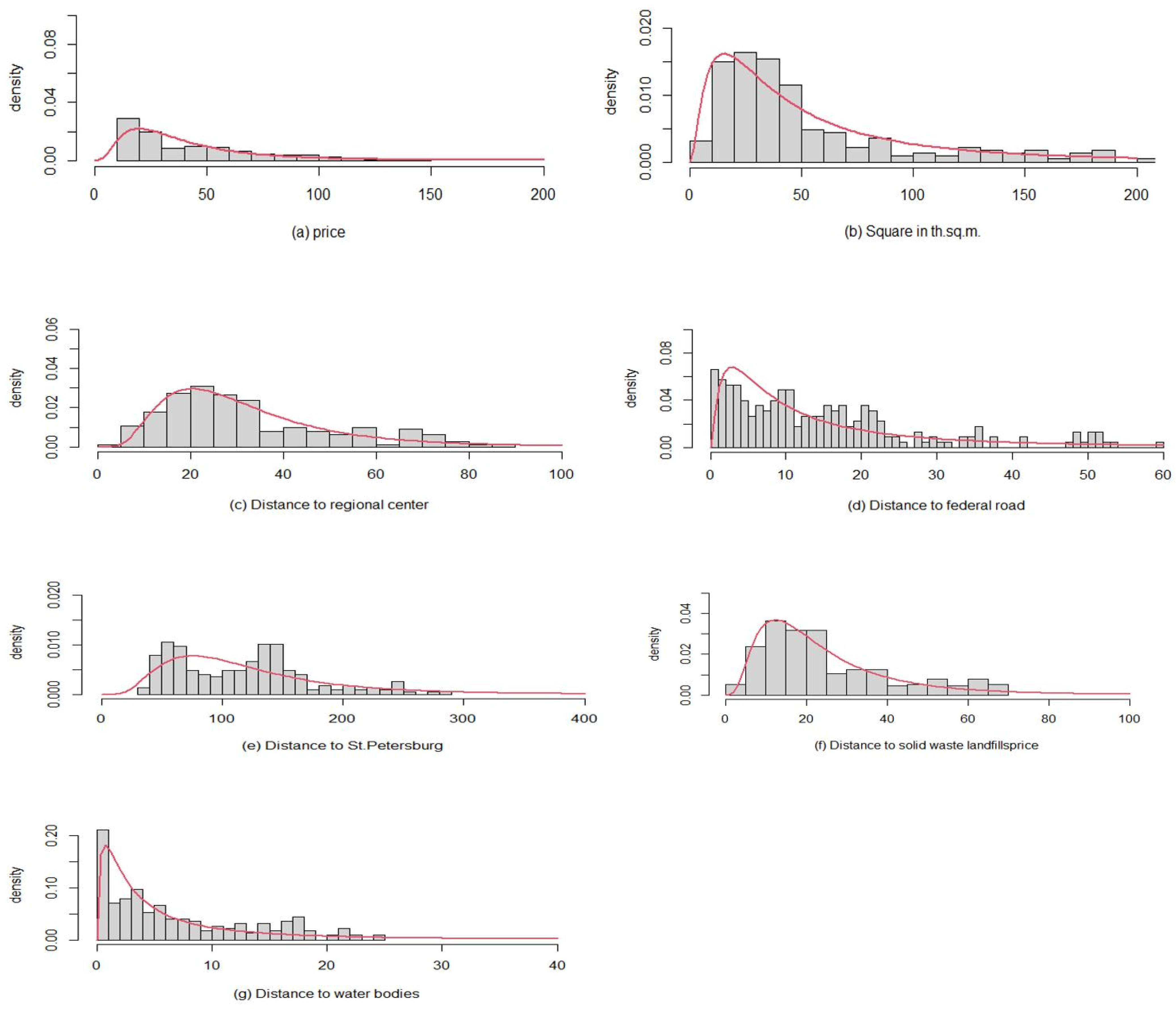
The units of measurement for the selected variables listed above are the following: all the listed distances are measured in kilometers, the area of the land plot is in thousands of meters, and the price is in rubles per 1 sqm of a land plot. For some of the empirically observed factors, such as the area of the object, the distance to roads of federal importance, the distance to the district center, the distance to major rivers and lakes, and the distance to landfills of solid waste, it is possible to construct acceptable fits with a lognormal distribution.

Figure 1 shows the distributions of the selected variables compared to the lognormal distribution.

The variable distance to St. Petersburg is not quite well fit for such a distribution and has a distinct double-modality (Figure 1). This can be explained by the smaller number of comparison objects at a distance of 70 to 130 km from a large federal center, and, apparently, reflects the real situation, because not all lands can be used for agricultural purposes. In addition, at such a distance, there are large water areas of the Gulf of Finland and Lake Ladoga. However, if in the places of ‘failure’ of distance distribution to St. Petersburg there could be agricultural land, the distribution would probably have a different form, as shown in Figure 1, where the red lines show the lognormal distributions.

For all seven examples in Figure 1 satisfactory p-values of Kolmogorov–Smirnov tests were obtained for normality as shown in

Table 1. p values for Kolmogorov–Smirnov test for normality.

Variable	p Value
price per 1 sqm of agricultural land plot in rubles	0.1857
land plot area	0.1513
distance to St. Petersburg	0.1003
distance to federal roads	0.156
distance to the district/regional center	0.4731
distance to major rivers and lakes	0.1071
distance to solid waste landfills	0.7018

. The satisfactory p value is the one with a value over 0.05 for accepting normality.

In general, the pricing factors expressed in units of distance do not have to obey the lognormal law of distribution, but a consistent and non-conflicting model of cadastral value formation is needed, in which natural trends of increase and decrease in value are formed when the values of the factors decrease or increase. The empirical distributions in Figure 1 are only marginal distributions (projections of the multidimensional scattering cloud on each of the coordinate axes), but we are more interested in the normality of the joint distribution of the logarithms of prices and price-generating factors.

4.2. Verification of Joint Lognormal Distribution

All of the above factors and prices are combined into a 7-dimensional vector, V, X₁, X₂, X₃, X₄, X₅, X₆, where

V is the price per 1 sqm of agricultural land plot in rubles;

X₁ is the area of the land plot in thousands of square meters;

X₂ is the distance to the district/regional center in kilometers;

X₃ is the distance to the federal road in kilometers;

X₄ is the distance to St. Petersburg in kilometers;

X₅ is the distance to solid waste landfills in kilometers;

X₆ is the distance to major rivers or lakes in kilometers.

When selecting objects for comparison, they were selected so that, in the resulting dataset, there were no objects with the same values for any factor. The unit of measurement might vary as the test for joint normality of seven coordinates (price, area, and five distances) uses a linear combination (weighted average) with random weights for all seven variables, and none of the variables can be allowed to dominate numerically over the others.

The possibility of using the Formula (5) or the Formulae (6) and (7) for the assessment of the market value of 1 sqm of land plot designed for agricultural production is determined by the possibility of accepting the hypothesis of lognormal distribution of the vector V, X₁, X₂, X₃, X₄, X₅, X₆, i.e., lognormal distribution is a prerequisite of the application of the formulae.

The following hypothesis tests the lognormal distribution.

H₀: 

The vector V, X₁, X₂, X₃, X₄, X₅, X₆ follows lognormal distribution.

To test this hypothesis, a bootstrap test of univariate distributions formed by arbitrary linear combinations of centered logarithms of vector components V, X₁, X₂, X₃, X₄, X₅, X₆ is performed.

The sequence of actions is as follows:

• The vector W, Y₁, Y₂, Y₃, Y₄, Y₅, Y₆ (W=ln(V), $Y_i=ln(X_i),i=\overline{1,6}$ ) is considered.
• The vector W, Y₁, Y₂, Y₃, Y₄, Y₅, Y₆ is centered.
• Seven random numbers—in total equal to 1—are generated.
• A random linear combination of the components W, Y₁, Y₂, Y₃, Y₄, Y₅, Y₆ is made.
• The empirical distribution of the obtained linear combination for correspondence to the theoretical lognormal law using the Kolmogorov–Smirnov test is checked.
• The previous three steps are repeated a sufficiently large number of times to see how many times the p-value of the Kolmogorov–Smirnov test is higher than the critical significance level of 0.05.

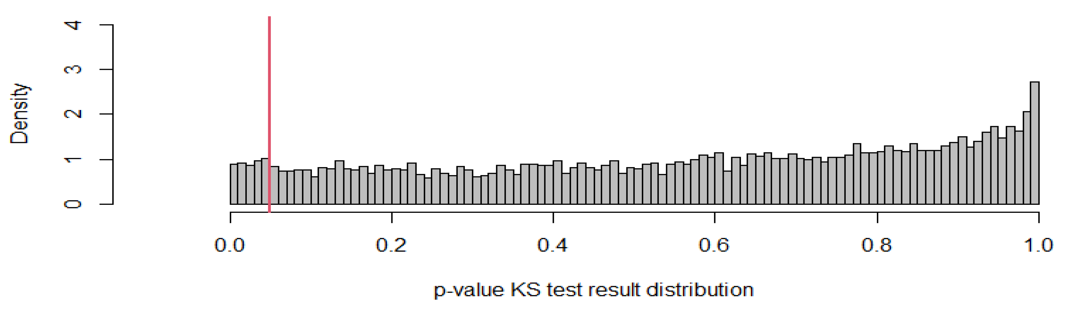
Figure 2 shows the results of bootstrap testing with the number of repetitions of univariate tests 10,000 times. On the horizontal line, the p-value of the one-time univariate Kolmogorov–Smirnov test to a random linear combination of the components of a multivariate vector is shown. The red line shows p = 0.05.

In 9531 cases out of 10,000, the p-value of the Kolmogorov–Smirnov test was greater than 0.05, which means 95.31%. We consider this to be a sufficient basis for using the Formula (5) (or (6) and (7)) to plot a consistent model of cadastral value as an estimate of the market value of land plots for agricultural production in the Leningrad region.

5. Application of the Theoretical Model

The application of the Formula (5) gives an estimate of the most typical land plot for agricultural production in the Leningrad region. Its parameters are given in

Table 2. Parameters to be used for the application of the theoretical model.

Variable Notation	Variable Name	Variable Value
V	price per 1 sqm of land for agricultural production	36 rubles
X1	land area is	17.54 thousand square meters
X2	distance to the district/regional center	15.09 km
X3	distance to the federal road	1.47 km
X4	distance to St. Petersburg	90.37 km
X5	distance to solid waste landfills	12.9 km
X6	distance to major rivers or lakes	0.99 km

.

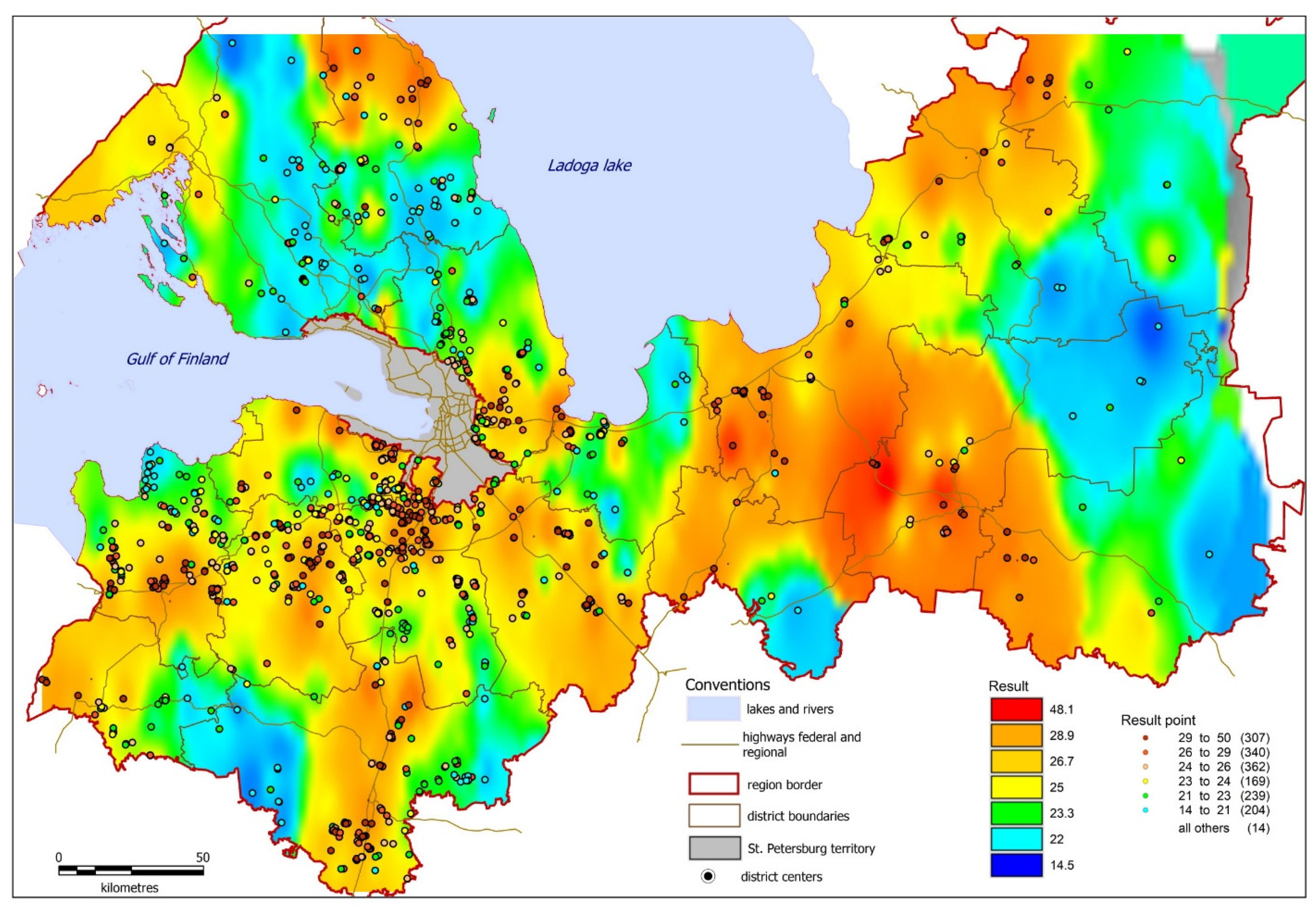
We are mostly interested in the assessment of the market value of one sqm land plot intended for agricultural production in the Leningrad region, which passed the cadastral registration, with a total number of 1635. In addition, the price of one sqm of land plot can be estimated, assuming that it could be intended for agricultural production—thus enabling a “heat map” of the entire region to be compiled (Figure 3).

Figure 3 shows the scale corresponding to the prices in the original set whose distribution is shown in Figure 1a, which presents that price distribution has a long right tail, i.e., rare but high prices are present in the initial data. Plots with such prices create a well “heated” zone on the “thermal” map of Figure 3, which corresponds to the typical behavior of market participants—if a plot is expensive, then its neighbors begin to evaluate their own plots as more expensive. However, as Figure 1a shows, there are a lot fewer such areas in the initial data than in the large-scale price area.

The heat map clearly depicts the areas of high- and low-cost land plots—red and yellow, respectively—which in turn, will show the areas where it is inexpedient to withdraw the land plots (high value) from agricultural cultivation and areas where such withdrawal due to low cost may be beneficial for other purposes (e.g., for green energy facilities), and cannot damage the regional agricultural production (low productivity resulting in a low price). The result is obtained in the statistical package R, applying Formula (5) to all such land plots entered in the cadastral database. Due to the large volume of data, the final result is displayed as a “heat” map of the Leningrad region (Figure 3).

The software program in which the heat map is built processes all the data in the original set. In the upper price range, there are few plots in the initial data, and expensive prices are separated from moderate and low prices at a greater distance than the ranges of low and moderate prices (this can be seen in Figure 1a). Therefore, the red interval captures a much larger range (all expensive prices, including the maximum price as well, fall here) than the intervals of the other colors representing lower prices.

Figure 3 also shows how much 1 sqm of land plot intended for agricultural production would cost at the corresponding location on the map. The dots show the position of the plots that passed cadastral registration as intended for agricultural production. The result in Figure 3 does not necessarily coincide with the results obtained by the cadastral office, due to the difference in the applied assessment methods, but this result looks highly consistent. The cost of 1 sqm land decreases with growing distance from the district centers, federal roads, and water bodies, with an increase in the area of the site while cost increases with the distance from solid waste landfills. In areas marked with colors from blue to yellow, the market value assessment is low. In these areas an alternative, more profitable use of land may be considered, for example, the placement of green energy facilities.

6. Discussion

Traditional evaluation methods in the comparative approach are based, as a rule, on small samples and techniques for adjusting the prices of objects of comparison or regression models built on a small number of observation points. These are the recognized methods based on which the formation of valuation activities in the Russian Federation took place to a large extent. From the point of view of the application of mathematical methods, the works [35,36,37] are considered classical.

In today’s environment, a much larger amount of market data (big data) are available and accessible, which requires different processing methods. One of the possible methods is the study of the entire datasets, the selection of model distributions, and the construction of estimates based on model distributions.

The present study proposes the development of a comparative approach, which is given much less attention in the valuation literature than the cost and income approaches, as, for example, in works [38,39,40]. At the same time, a comparative approach can give an adequate picture of the current state of the market. The comparative approach and analysis of big market data require special and careful attention, since there are two extremes in the market data; on the one hand, there can be a large amount of “garbage data” in the datasets, and, on the other hand, even with a large amount of data, information about pricing factors can be extremely limited (as in our case).

The suggested research method is proposed as one of the possible options for assessing the market value of real estate objects (which include land plots) based on a large amount of comparative data, in the absence of information about pricing factors, using geographic information systems data.

We propose one of the possible methods, namely the study of the entire set of data, the selection of model distributions, and the construction of estimates based on model distributions. The data obtained from geoinformation systems make it possible to interpret all used pricing factors as real (continuous) and build estimates based on hypotheses about the type of joint distribution of observed values.

Of course, each time it is necessary to check the observed values for compliance with one or another type of distribution. There are a priori justifications for the log-normal distribution, but perhaps other kinds of distributions can be observed. Empirical distributions always differ from model ones. The question is how well empirical distributions follow model distributions and whether the results obtained satisfy the ultimate goal of the study. In the present case, a somewhat loose use of the empirical distribution for the distance to St. Petersburg still gives a certain model that allows for the determination of the most probable price value (market value).

If some of the pricing factors are rank factors, the set of initial data can be divided into subsets with the same rank values and then, if there is enough data in each subset, a similar research method with continuous pricing factors can be applied. Factors are determined based on geoinformation databases (distance to the nearest large city, regional center, federal highway, large rivers, lakes, and solid waste landfills), which allow a market assessment in the absence of information on pricing factors for land plots, except for the offer price and the plot area.

The problem of market valuation is being solved in the conditions of the almost complete absence of information about price-forming factors in the areas being assessed. The present study was made in need to determine on a specific date the cadastral value of agricultural land for the purposes of taxation, corresponding to the market value, in the almost complete absence of information on pricing factors in the assessed areas.

7. Conclusions

The goals of sustainable development are fundamentally consistent. However, the economic activity of hundreds of thousands of economic agents that operate in competitive markets inevitably results in conflicts of various kinds, which ultimately affect the sustainability of economic systems as a whole.

The mathematical toolkit proposed in this work is aimed at minimizing the negative consequences of those decisions in the land use sector that were potentially made without a sufficiently objective approach due to various kinds of circumstances. This toolkit is also the basis for a consistent model of cadastral value as an assessment of the market value of land plots for agricultural production. Another distinctive aspect of our proposed approach is the possibility of determining the boundaries of high and low values of land plots, which in turn will show the areas where it is inexpedient to withdraw the land (high value) and areas where, due to low value, such withdrawal can be beneficial for other purposes (for example, to accommodate green energy facilities) and not harm the regional agricultural production.

The proposed approach is also supported by the widespread use of geographic information systems, which generate extensive information on the condition of various land areas. Such information, thanks to the proposed mathematical toolkit, makes it possible to carry out a mass evaluation of land plots when allocating land for green energy facilities and evaluating agricultural plots.

The proposed approach can be widely used in assessing since geographic information systems are available and inexpensive. The widespread use of digital technologies can give us certain optimism that this factor cannot be a barrier. At the same time, the approach proposed in the paper can give impetus to the development of new methods for alternative estimates of land use in the framework of sustainable development.