Preference and Stability Regions for Semi-Implicit Composition Schemes

Abstract

A numerical stability region is a valuable tool for estimating the practical applicability of numerical methods and comparing them in terms of stability. However, only a little information can be obtained from the stability regions when their shape is highly irregular. Such irregularity is inherent to many recently developed semi-implicit and semi-explicit methods. In this paper, we introduce a new tool for analyzing numerical methods called preference regions. This allows us to compare various methods and choose the appropriate stepsize for their practical implementation, such as stability regions, but imposes stricter conditions on the methods, and therefore is more accurate. We present a thorough stability and preference region analysis for a new class of composition methods recently proposed by F. Casas and A. Escorihuela-Tomàs. We explicitly show how preference regions, plotted for an arbitrary numerical integration method, complement the conventional stability analysis and offer better insights into the practical applicability of the method.

1. Introduction

One of the key problems in numerically solving initial value problems (IVP) is constructing an integration scheme that is suitable for obtaining an accurate numerical solution as quickly and reliably as possible. In recent years, many novel efficient numerical methods have been presented [1,2,3,4]. The composition and splitting schemes are of great interest at present, being applied to problems with oscillatory solutions and especially to conservative problems [5,6,7,8,9,10]. The fact that composition methods allow for an increase in the accuracy order of basic methods while simultaneously saving their geometric properties provides researchers with a powerful experimentation tool. Some of the newest approaches in the considered field of splitting and composition schemes [11] are still not provided with a general analysis of their numerical stability, which raises questions about the actual performance of the proposed schemes and their applicability to real problems. The numerical stability of composition schemes heavily relies on the geometric properties of the basic low-order method. Recently proposed generalized semi-implicit and semi-explicit numerical methods [12] were proven to be reliable and effective basic integrators for composition schemes, combining the simplicity and computational efficiency of explicit methods with the higher numerical stability of implicit methods.

The traditional approach to evaluating numerical methods’ stability assumes the plotting of so-called stability regions: areas of the complex plane where a linear test problem possesses stable solutions. This type of analysis has proven to be reliable for comparing various methods and concluding whether the investigated method has some special stability properties that are useful for specific problems [13]. Nevertheless, this approach often does not take into account the simple fact that a part of the obtained stability region is practically useless. While the solution in this part is stable, its behavior is far from the original behavior of the prototype continuous system. In other words, the numerical error can be too high to consider the solution practically useful in this case. This drawback of the stability region analysis is negligible in the case of most conventional numerical methods with relatively simple shapes of the stability regions but makes such an analysis poorly applicable when numerical methods possess more complicated stability regions. Excellent examples of such methods are semi-implicit and semi-explicit methods [14]. In the case of composition methods based on semi-implicit and semi-explicit integrators, the situation becomes even more complicated, as we show in the current study. In this paper, we propose a new tool for stability analysis called preference regions. The preference region of the numerical method is a region in the complex plane where the solution of a linear test problem is stable and the local relative error of the solution does not exceed one. A stricter definition will be given in Section 2.2. The goal of this study is to develop a novel technique to perform an analysis of the numerical stability of numerical methods and show its application to state-of-the-art composition integration methods. The subject of our investigation is a family of composition schemes recently proposed by F. Casas et al. [11], which have not yet been thoroughly analyzed for their numerical stability and applicability to non-conservative problems. We examine these schemes using semi-implicit and semi-explicit integrators as basic methods. We will also analyze their general performance in comparison with completely implicit schemes and discuss the advantages of the new approach to stability evaluation in combination with an accuracy analysis of the obtained solution.

2. Materials and Methods

2.1. Stability Regions

Initially proposed by Dahlquist and further adopted by other authors, the stability region of the numerical method is a region in the complex plane defined as follows [13]. Let us consider a standard test problem

$$\dot{x}=\lambda x,$$

(1)

where $\lambda$ is a complex number. Applying any single-step numerical method to this problem with a stepsize $h$ yields a relation

$$x_{n+1}=R\left(h\lambda \right)x_n.$$

(2)

Once we denote $h\lambda =z$, the part of the complex plane where $\left|R\right(z\left)\right|\le 1$ is a stability region.

One way to numerically evaluate the stability of semi-explicit and semi-implicit methods is to use a technique based on the approach with test problems of dimension 2 [15], which is somehow similar to the technique using the Dahlquist test problem [16] but allows one to calculate stability regions of methods which does not exist for one-dimensional problems. Let us consider a two-dimensional autonomous test problem with matrix $A$:

$$\dot{x}=Ax,A=\left(\begin{array}{cc}a& b\\ c& d\end{array}\right).$$

(3)

After applying an integration method, a two-dimensional difference equation can be derived similarly to Equation (2):

$$x_{n+1}=R\left(ah,bh,ch,dh\right)x_n$$

(4)

Complex conjugate eigenvalues of the presented matrix $A$ define the dynamics of the solution of the chosen test problem and can be written as:

$${\lambda }_{12}=\sigma \pm j\omega .$$

Let us denote two free parameters, $r\ge 0$ and $k\ge 0$, which define the eccentricity and asymmetry of the matrix $A$:

$$\begin{array}{c}a=kd,\hfill \\ b=rc,\hfill \\ c=-\sqrt{\frac{1}{r}\left({\lambda }_1^2-\left(1+k\right)d{\lambda }_1+k{d}^2\right)},\hfill \\ d=\frac{2\sigma }{1+k}.\hfill \end{array}$$

(5)

Asymmetry coefficient $k$ defines the shape of the stability region, maximizing it at $k=1$, which turns the matrix into the Jordan normal form, and minimizing it at $k=0$ or $k=\infty$, which turns the matrix into the Frobenius normal form. When discussing the two-dimensional problem, we should mention that, in this case, the stability region is the area in the complex plane where the absolute values of the complex conjugate eigenvalues of the matrix $R$ from Equation (4) are not greater than 1. The parameter $r$ has no impact on the shape of the stability region and is set to unity.

2.2. Preference Regions

By analyzing the stability regions of any numerical integration scheme, either implicit, explicit, or partially implicit, one can come to the simple conclusion that A-stable methods, such as the implicit middle point, might be excessive for most of the regular nonlinear IVPs when the accuracy requirements are relatively high. In this case, the vast majority of the stability region does not contribute to the sufficient accuracy of the solution. While the solution might prove to be stable, the high levels of local truncation errors will barely allow for it to be used in any real application.

One can observe such a phenomenon by developing a mathematical model for testing different values taken from the stability region and outside of it over the complex plane. Then, the model needs to be compared with the reference one, providing the researcher with an error graph from which one may judge the accuracy of the model. For example, by analyzing the stability region of the explicit Euler method, one can see that simulation results highly depend on the point in the complex plane where the next step of the method is calculated (Figure 1 and Figure 2). In this example, the linear system has a matrix with coefficients (5) determined by the position of complex conjugate eigenvalues and the initial conditions are (10; −2).

Figure 2 illustrates the various behaviors of the solutions. Solutions in points (a) and (c) are unstable, as predicted by the position of the points relative to the stability region. The solution (b) is oscillatory since point (b) is on a boundary of the stability region. All these solutions are obviously erroneous relative to the continuous prototype. Solutions obtained in points (d), (e), (g), and (h), which lie within the stability region, show dynamics that are also rather far from the real dynamics of the prototype system. Only the solutions in cases (f) and (i) are somewhat close to the real dynamics of the continuous system with respect to the truncation error. As expected, the error in (i) is lower than in (f) because (i) is closer to the origin than (f). This example clearly shows the importance of a technique that will be able to evaluate areas in the complex plane within the stability region where the investigated method is better-suited to providing the most precise numerical solution.

2.3. The New Technique of Preferable Stability Regions Evaluation

As demonstrated in a previous section, while the obtained solution may be stable it can simultaneously be inaccurate. One may perform a subsequent experiment to evaluate the feasibility of using the numerical method to solve the problem at the current point of the complex plane by comparing the obtained solution with an accurate solution using the following formula:

$$err=\frac{x_n-x_n^{acc}}{x_n^{acc}},$$

(6)

where $x_n$ represents the solution obtained with the given method and $x_n^{acc}$ represents an accurate solution of a proposed system, which can unambiguously be found at the exact moment of time h using the matrix exponential:

$$x_n^{acc}=e^{Ah}{x}_{n-1}.$$

Thus, by comparing the obtained coefficient $err$ with any chosen tolerance value, one can judge the applicability of the chosen method for solving the given IVP. From this, a definition of preference region follows.

Definition 1.

The preference region of the numerical method is a region in the complex plane where the solution of the test problem (1) or (3) is stable, i.e., $\left|\mathrm{eig}\left(R\right)\right|\le 1$, and the relative error (6) satisfies an inequality $\left|err\right|\le 1$.

While plotting the preference region is as simple as plotting the stability region, the algorithm in the pseudocode for the one-dimensional test problem is given as Algorithm 1 for the reader’s convenience. The symbol $\mathrm{𝕚}$ denotes an imaginary unit to avoid confusing a loop-counter.

Algorithm 1: Plotting preference region for the one-dimensional test problem

Input: bounds ${\sigma }_{min}, {\sigma }_{max}, {\omega }_{min},{\omega }_{max}$, grid stepsizes $\mathsf{\Delta }\sigma ,\mathsf{\Delta }\omega$

Output: preference region image $R_{pref}$

$X,Y\leftarrow meshgrid\left({\sigma }_{min}:\mathsf{\Delta }\sigma :{\sigma }_{max},{\omega }_{min}:\mathsf{\Delta }\omega :{\omega }_{max}\right)$

$nd\leftarrow size\left(X\right)$

$R_{pref}\leftarrow zeros\left(n{d}_1,n{d}_2\right)$

for $i\in 1..n{d}_1$

for $j\in 1..n{d}_2$

$\sigma \leftarrow X_{ij}$

$\omega \leftarrow Y_{ij}$

$z\leftarrow \sigma +\mathrm{𝕚}\omega$

$R_{prec}\leftarrow e^z$ //this is a precise solution

$R_{stab}\leftarrow R\left(z\right)$ //this is a stability function

$R_{pref}\left(i,j\right)\leftarrow \frac{\Vert R_{prec}-R_{stab}\Vert }{\Vert R_{prec}\Vert }<1$

end

end

Algorithm 2 summarizes the same set of operations for two- and multi-dimensional test problems.

Algorithm 2: Plotting preference region for the multi-dimensional test problem

Input: bounds ${\sigma }_{min}, {\sigma }_{max}, {\omega }_{min},{\omega }_{max}$, grid stepsizes $\mathsf{\Delta }\sigma ,\mathsf{\Delta }\omega$, asymmetry coefficient k

Output: preference region image $R_{pref}$

$X,Y\leftarrow meshgrid\left({\sigma }_{min}:\mathsf{\Delta }\sigma :{\sigma }_{max},{\omega }_{min}:\mathsf{\Delta }\omega :{\omega }_{max}\right)$

$nd\leftarrow size\left(X\right)$

$R_{pref}\leftarrow zeros\left(n{d}_1,n{d}_2\right)$

for $i\in 1..n{d}_1$

for $j\in 1..n{d}_2$

$\sigma \leftarrow X_{ij}$

$\omega \leftarrow Y_{ij}$

$d\leftarrow \frac{2\sigma }{1+k}$

$\lambda \leftarrow \sigma +\mathrm{𝕚}\omega$

$A\leftarrow \left(\begin{array}{cc}kd& -\sqrt{{\lambda }_1^2-\left(1+k\right)d{\lambda }_1+k{d}^2}\\ \sqrt{{\lambda }_1^2-\left(1+k\right)d{\lambda }_1+k{d}^2}& d\end{array}\right)$

$R_{prec}\leftarrow e^A$ //this is a precise solution

$R_{stab}\leftarrow R\left(A\right)$ //this is a stability function

$R_{pref}\left(i,j\right)\leftarrow \frac{\Vert R_{prec}-R_{stab}\Vert }{\Vert R_{prec}\Vert }<1$

end

end

The proposed technique can be used with a variety of different numerical integration methods, including composition schemes and the methods of the Runge–Kutta (RK) family (Figure 3).

One can see that the size of the stability regions of the Runge–Kutta methods correspond well with the size of their preference regions. However, this example does not illustrate the real motivation for introducing the preference regions. A more interesting example is given in Figure 4, where the stability and preference regions of the implicit RK methods are plotted.

In Figure 4, RK1 denotes the implicit Euler method. RK2 is the implicit midpoint rule and RK4 is the fourth-order Lobatto IIIC method. One can see that while all these methods are A-stable, which means that the entire left half-plane belongs to the stability region, only a minor part of this region is practically useful in terms of acceptable error. Moreover, the shape of preference regions is highly irregular, resembling the order stars of numerical methods [13]. Let us apply the preference region analysis to a recently reported class of composition numerical methods.

2.4. Composition Schemes

In the foundational work of H. Yoshida [18], the general principles of constructing high-order symplectic integrators by the composition of low-order basic methods were presented. The proposed technique allows for one to achieve an approximation of higher order by combining solutions obtained by the basic single-step method ${\mathsf{\Phi }}_h$ in the following way. First, one must choose numbers ${\gamma }_1,\dots ,{\gamma }_s$, so that they satisfy the following consistency condition:

$${\gamma }_1+{\gamma }_2+\dots +{\gamma }_s=1.$$

Then, one will be able to obtain a composition method with s stages:

$${\mathsf{\Psi }}_h={\mathsf{\Phi }}_{{\gamma }_{s}h}\circ \cdots \circ {\mathsf{\Phi }}_{{\gamma }_{2}h}\circ {\mathsf{\Phi }}_{{\gamma }_{1}h}.$$

For three stages of composition, an example of such coefficients is:

$$\begin{gathered} {\gamma }_1={\gamma }_3={\left(2-2^{\frac{1}{p+1}}\right)}^{-1}, \\ {\gamma }_2=-2^{\frac{1}{p+1}}{\left(2-2^{\frac{1}{p+1}}\right)}^{-1}, \end{gathered}$$

where p is the accuracy order of the basic method ${\mathsf{\Phi }}_h$.

Various techniques for obtaining the coefficients ${\gamma }_1,\dots ,{\gamma }_s$ were presented by different authors, which yielded a great variety of numerical methods. In the field of composition schemes, the outstanding works by Kahan and Li [19] and more recent research by F. Casas et al. [20] are of great interest. In these studies, the authors implemented efficient schemes aiming to minimize large high-order error terms that appeared in classical composition methods.

2.4.1. Composition Scheme of Kahan and Li

A proposition by Kahan and Li [19] directly followed the work of Yoshida, which mainly aimed to suppress a large, high-order error term via minimization

$$\underset{1\le i\le s}{ \max }\left|{\gamma }_i\right| \mathrm{and} {\displaystyle \sum }_{i=1}^s\left|{\gamma }_i\right|,$$

where s is the number of stages.

The composition coefficients proposed by Kahan and Li [19] are applicable to schemes that use symmetric and self-adjoint basic methods. Some of these coefficients, which we use in our research, are presented in

Table 1. Coefficients for composition schemes of different orders and number of stages.

s1ord2
γ1	1
s3ord4
${\gamma }_1={\gamma }_3$	1.3512071919596578
${\gamma }_2$	−1.7024143839193155
s5ord4
${\gamma }_1={\gamma }_2={\gamma }_4={\gamma }_5$	0.414490771794375737142354063
${\gamma }_3$	−0.65796308717750294856941625
s7ord6
${\gamma }_1={\gamma }_7$	0.78451361047755726382
${\gamma }_2={\gamma }_6$	0.23557321335935813368
${\gamma }_3={\gamma }_5$	−1.1776799841788710069
${\gamma }_4$	1.3151863206839112189
s15ord8
${\gamma }_1={\gamma }_9$	0.39103020330868478817
${\gamma }_2={\gamma }_8$	0.33403728961113601749
${\gamma }_3={\gamma }_7$	−0.70622728118756134346
${\gamma }_4={\gamma }_6$	0.08187754964805944576890
${\gamma }_5$	0.79856447723936218406

, with identical notationl to the original article, i.e., s3ord4 denotes a scheme with three stages, which delivers an approximation of the fourth order.

2.4.2. Approach by Casas and Escorihuela-Tomàs

In their recent work, F. Casas and A. Escorihuela-Tomàs proposed a new technique for minimization of the high-order error terms [11]. The developed approach generally aimed to solve nonlinear problems separable into three parts [20], but it also appeared to be efficient for solving a more general class of IVPs when using appropriate basic methods with low computational costs, e.g., semi-implicit and semi-explicit integrators.

Some of the coefficients found for fourth-order composition schemes, which are used in this paper, are presented in

Table 2. Coefficients for composition schemes of fourth order with different number of stages.

$X{A}_4$
${\gamma }_1$ = 0.358	${\gamma }_3$ = 0.35230499471528197958
${\gamma }_2$ = −0.47710242361717810834	${\gamma }_4$ = 0.26679742890189612876
$X{A}_5$
${\gamma }_1={\gamma }_2={\gamma }_3={\gamma }_4$ = 0.20724538589718786
${\gamma }_5$ = −0.3289815435887514
$X{A}_6$
${\gamma }_1$ = 0.16	${\gamma }_4$ = −0.260672267225
${\gamma }_2$ = 0.15	${\gamma }_5$ = 0.147945412322
${\gamma }_3$ = 0.16	${\gamma }_6$ = 0.142726854903
$X{B}_4$
${\gamma }_1$ = 0.1728230091083	${\gamma }_3$ = −0.574223836304
${\gamma }_2$ = 0.4307494176206	${\gamma }_4$ = 0.4706514095751
$X{B}_5$
${\gamma }_1$ = 0.08967664078837	${\gamma }_4$ = −0.4942190871723
${\gamma }_2$ = 0.1603233592116	${\gamma }_5$ = 0.4478961696306
${\gamma }_3$ = 0.2963229175417

under the notation of $X{A}_s$, where s is the number of composition stages.

As stated by the authors of the original article [11], one can use the proposed coefficients with an arbitrary first-order method and its adjoint to compose numerical schemes of higher-accuracy orders.

2.5. Basic Methods Used in Composition Schemes

2.5.1. Semi-Implicit CD Method

The semi-implicit integration CD method, which is a generalization of the Störmer–Verlet method over the arbitrary separable IVP, was previously described in [12] and is chosen as a basic method for the proposed composition schemes as it possesses high computational efficiency [21]. Due to its semi-implicit calculation nature, it exists only for ODE systems of order two and higher. Let us consider the following IVP:

$$\{\begin{array}{c}\dot{x}=f\left(x,y,t\right)\\ \dot{y}=g\left(x,y,t\right)\end{array},$$

(7)

with initial conditions $x\left(t_0\right)=x_0, y\left(t_0\right)=y_0$. A semi-implicit algorithm can be described as a composition of two adjoint methods forming a symmetric scheme of the second accuracy order:

$$\mathsf{Ф}\left(x_n,y_n,h,t_n\right):\{\begin{array}{c}\begin{array}{c}{x}_{n+0.5}=x_n+\frac{h}{2}f\left(x_n,y_n,t_n\right)\\ y_{n+0.5}=y_n+\frac{h}{2}g\left(x_{n+0.5},y_n,t_n\right)\end{array}\\ y_{n+1}=y_{n+0.5}+\frac{h}{2}g\left(x_{n+0.5},y_{n+1},t_{n+1}\right)\\ x_{n+1}=x_{n+0.5}+\frac{h}{2}f\left(x_{n+1},y_{n+1},t_{n+1}\right)\end{array},$$

which can be rewritten as a semi-explicit scheme by changing the order of explicit and implicit counterparts in the composition.

2.5.2. Implicit Midpoint Method

An implicit midpoint method is one of the most well-known symplectic integrators and is often used in composition schemes. The solution to the IVP (7) requires two calls to the right-side function (RHS) and can be described by the following formula:

$$\widetilde{\mathsf{Ф}}\left(x_n,y_n,h,t_n\right):\{\begin{array}{c}{x}_{n+1}=x_n+hf\left(\frac{x_n+x_{n+1}}{2},\frac{y_n+y_{n+1}}{2},t_{n+0.5}\right)\\ y_{n+1}=y_n+hg\left(\frac{x_n+x_{n+1}}{2},\frac{y_n+y_{n+1}}{2},t_{n+0.5}\right)\end{array}.$$

Implicit calculations are conducted by applying Newton’s method to every approximation of state variables, $x_n,y_n$ in the case of IVP (7). This provides a better numerical stability while solving Hamiltonian test problems but is significantly less efficient than explicit and semi-implicit methods in terms of time and computational costs. We will use the implicit midpoint method as one of the basic integrators in the investigated composition schemes.

3. Results

Stability regions and preference regions obtained for the investigated composition schemes (Table 2), with semi-implicit CD and implicit midpoint methods chosen as a basic method, are given in this section in Figure 5, Figure 6, Figure 7, Figure 8 and Figure 9.

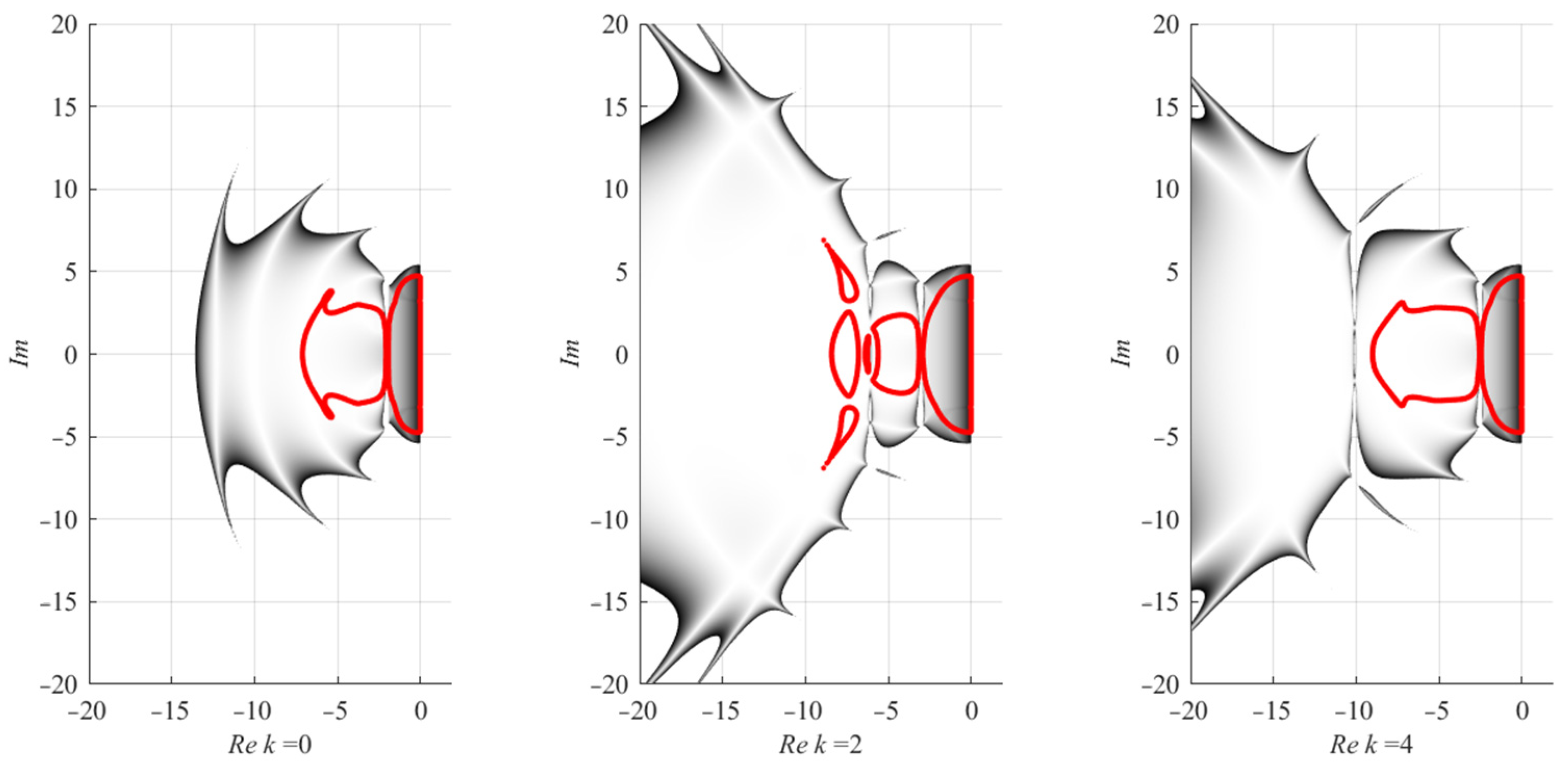
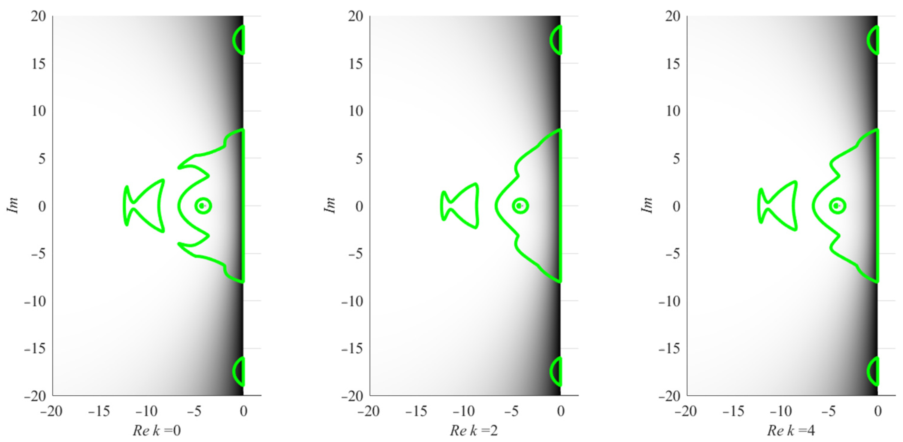
The main observation, which can be made by analyzing the results shown in Figure 5, Figure 6, Figure 7, Figure 8 and Figure 9, is that, while the considered schemes may have significantly high stability, the region on a complex plane, in which the solution can be considered reasonably accurate, is much smaller. Semi-implicit schemes, while being less stable than their fully implicit counterparts, demonstrate a reasonable tradeoff between stability and computation efforts since their preference regions are not as small as their stability regions. In addition, semi-implicit schemes do not require Newton iterations because the one-dimensional implicitness can be resolved analytically or by using the simple iterations method.

One can see that stability and preference regions generation for implicit midpoint schemes are of particular interest because they both bypass one special point on a complex plane, while the results obtained for semi-implicit CD schemes do not represent such behavior. In real applications, this fact can limit the applicability of the implicit midpoint method as a basic integrator for composition schemes.

Typically, preference regions consist of multiple areas over the complex plane, which have distinct empty spaces in between, where the solution is not accurate and therefore cannot be used. The main area of interest starts from 0 on the real axis and spreads onto the negative half-plane. Empirically, one can conclude that the wider this area is, the better the overall performance of the proposed method will be in terms of both the accuracy and stability of the solution.

Evaluating the results of the performed analysis, one may come to a general conclusion that using implicit basic methods can be considered less efficient than it is usually claimed to be if one takes into account only stability regions that occupy the entire left half-plane. A region that is suitable for practical use in mathematical modeling is much smaller in size than its counterpart in semi-implicit schemes. The analysis shows that semi-implicit modifications of composition methods are expected to be efficient in terms of both stability and precision due to their higher general stability and that the regions that are suitable for obtaining correct solutions are large enough.

4. Conclusions and Discussion

The reported study is dedicated to preference regions, a novel tool for the analysis of numerical integration methods’ performance and its application to newly developed composition schemes based on semi-implicit methods. The proposed technique provides a general performance analysis of an integration scheme based on its local error and stability, allowing for one to choose the integration algorithm and stepsize in accordance with the simulated problem. Six conventional Runge–Kutta type schemes and five various novel composition schemes with implicit and semi-implicit basic methods were studied. The novel investigated schemes were taken from a recently reported study on methods of solving systems separable into three parts and applied to general-type initial value problems. The experimental data for the reported schemes were obtained using the two-dimensional test problem.

The obtained results show that conventional stability analysis of implicit schemes overestimates regions that are of practical interest, while less popular semi-implicit schemes can also provide reasonable stability due to the size and shape of the preference regions. This overestimation of the practically acceptable region in the complex plane is inherent to the stability region analysis itself and, therefore, might confuse the researchers, especially in the case of A-stable implicit methods, since the entire left half-plane belonging to a stability region makes an erroneous impression that each point in this half-plane can be involved in the real computation. Using preference region analysis, this error is easily avoided. However, this observation requires new, deeper insight into the better performance of implicit schemes, which is observed in practice for stiff problems. As this topic has not been at the cutting edge of computational mathematics for a long time, a full consensus on the issue of stiffness and stability has not been reached to date.

Further studies will be dedicated to an extension of the proposed preference region evaluation technique over a wider range of numerical methods and multistep integration schemes popular in the field of nonlinear dynamics. We also aim to develop more of the theoretical background on the problem of stiffness and stability with newly obtained results.

References

- Cavoretto, R.; De Rossi, A.; Mukhametzhanov, M.S.; Sergeyev, Y.D. On the search of the shape parameter in radial basis functions using univariate global optimization methods. J. Glob. Optim. 2021, 79, 305–327. [Google Scholar] [CrossRef]
- Paulavičius, R.; Sergeyev, Y.D.; Kvasov, D.E.; Žilinskas, J. Globally-biased BIRECT algorithm with local accelerators for expensive global optimization. Expert Syst. Appl. 2020, 144, 113052. [Google Scholar] [CrossRef]
- Kovács, E. A class of new stable, explicit methods to solve the non-stationary heat equation. Numer. Methods Partial. Differ. Equ. 2021, 37, 2469–2489. [Google Scholar] [CrossRef]
- Nadeem, M.; He, J.-H. He–Laplace variational iteration method for solving the nonlinear equations arising in chemical kinetics and population dynamics. J. Math. Chem. 2021, 59, 1234–1245. [Google Scholar] [CrossRef]
- Blanes, S.; Casas, F.; Chartier, P.; Escorihuela-Tomàs, A. On symmetric-conjugate composition methods in the numerical integration of differential equations. Math. Comput. 2022, 91, 1739–1761. [Google Scholar] [CrossRef]
- Roulet, J.; Choi, S.; Vaníček, J. Efficient geometric integrators for nonadiabatic quantum dynamics. II. The diabatic repre-sentation. J. Chem. Phys. 2019, 150, 204113. [Google Scholar] [CrossRef] [PubMed]
- Bréhier, C.E.; Goudenège, L. Weak convergence rates of splitting schemes for the stochastic Allen–Cahn equation. BIT Numer. Math. 2020, 60, 543–582. [Google Scholar] [CrossRef]
- Hansen, E.; Ostermann, A. High order splitting methods for analytic semigroups exist. BIT Numer. Math. 2009, 49, 527–542. [Google Scholar] [CrossRef]
- Wang, B.; Zhao, X. Error estimates of some splitting schemes for charged-particle dynamics under strong magnetic field. SIAM J. Numer. Anal. 2021, 59, 2075–2105. [Google Scholar] [CrossRef]
- Goth, F. Higher order auxiliary field quantum Monte Carlo methods. J. Phys. Conf. Ser. 2022, 2207, 012029. [Google Scholar] [CrossRef]
- Casas, F.; Escorihuela-Tomàs, A. Composition methods for dynamical systems separable into three parts. Mathematics 2020, 8, 533. [Google Scholar] [CrossRef]
- Butusov, D.; Tutueva, A.; Fedoseev, P.; Terentev, A.; Karimov, A. Semi-Implicit Multistep Extrapolation ODE Solvers. Mathematics 2020, 8, 943. [Google Scholar] [CrossRef]
- Wanner, G.; Hairer, E. Solving Ordinary Differential Equations II; Springer: Berlin/Heidelberg, Germany; New York, NY, USA, 1996; Volume 375. [Google Scholar]
- Tutueva, A.; Butusov, D. Stability Analysis and Optimization of Semi-Explicit Predictor–Corrector Methods. Mathematics 2021, 9, 2463. [Google Scholar] [CrossRef]
- Butusov, D.; Ostrovskii, V.Y.; Karimov, A.I.; Andreev, V.S. Semi-Explicit Composition Methods in Memcapacitor Circuit Simulation. Int. J. Embed. Real Time Commun. Syst. 2019, 10, 37–52. [Google Scholar] [CrossRef]
- Hairer, E.; Hochbruck, M.; Iserles, A.; Lubich, C. Geometric Numerical Integration. Oberwolfach Rep. 2006, 3, 805–882. [Google Scholar] [CrossRef]
- Dormand, J.R. Numerical Methods for Differential Equations: A Computational Approach, 1st ed.; CRC Press: Boca Raton, FL, USA, 1996; pp. 82–84. [Google Scholar]
- Yoshida, H. Construction of higher order symplectic integrators. Phys. Lett. A 1990, 150, 5–7. [Google Scholar] [CrossRef]
- Kahan, W.; Li, R.C. Composition constants for raising the orders of unconventional schemes for ordinary differential equations. Math. Comput. 1997, 66, 1089–1099. [Google Scholar] [CrossRef]
- Skokos, C.; Gerlach, E.; Bodyfelt, J.; Papamikos, G.; Eggl, S. High order three part split symplectic integrators: Efficient techniques for the long time simulation of the disordered discrete nonlinear Schrödinger equation. Phys. Lett. A 2014, 378, 1809–1815. [Google Scholar] [CrossRef]
- Butusov, D. Adaptive Stepsize Control for Extrapolation Semi-Implicit Multistep ODE Solvers. Mathematics 2021, 9, 950. [Google Scholar] [CrossRef]