Learning Adaptive Spatial Regularization and Temporal-Aware Correlation Filters for Visual Object Tracking

Abstract

Recently, discriminative correlation filters (DCF) based trackers have gained much attention and obtained remarkable achievements for their high efficiency and outstanding performance. However, undesirable boundary effects occur when the DCF-based trackers suffer from challenging situations, such as occlusion, background clutters, fast motion, and so on. To address these problems, this work proposes a novel adaptive spatial regularization and temporal-aware correlation filters (ASTCF) model to deal with the boundary effects which occur in the correlation filters tracking. Firstly, our ASTCF model learns a more robust correlation filter template by introducing spatial regularization and temporal-aware components into the objective function. The adaptive spatial regularization provides a more robust appearance model to handle the large appearance changes at different times; meanwhile, the temporal-aware constraint can enhance the time continuity and consistency of this model. They make correlation filters model more discriminating, and also reduce the influence of the boundary effects during the tracking process. Secondly, the objective function can be transformed into three sub-problems with closed-form solutions and effectively solved via the alternating direction method of multipliers (ADMM). Finally, we compare our tracker with some representative methods and evaluate using three different benchmarks, including OTB2015, VOT2018 and LaSOT datasets, where the experimental results demonstrate the superiority of our tracker on most of the performance criteria compared with the existing trackers.

1. Introduction

Visual tracking [1,2,3,4,5] plays a very important role in machine vision field and has been applied in many realistic scenes, including robots, traffic surveillance, self-driving cars, criminal investigation, and so on. It aims to predict the position and size of a tracked object with a bounding box in each frame, by employing a tracking method, where the position and size information is given in the first frame of each sequence. Although many advanced tracking methods [6,7,8] have been proposed in recent years due to the rapid development of computer sciences, many methods still have their weakness, including accuracy and robustness, speed and practicability in some specific scenes. Therefore, there are also lots of challenges urgently needing to be address.

Due to a high speed and a good performance, the DCF-based tracking method [9,10,11,12] has gained lots of attention, and various algorithms have been proposed in recent years. Traditional correlation filters (CF) based methods perform well both on accuracy and speed because of the usage of a circular shift operation. Thus, the training samples can be obtained using a circulant matrix and correlation filters can be optimized and solved in frequency domain by the fast Fourier transform (FFT). The CF-based tracking methods can be efficiently divided into background and object regions by learning a strong and discriminative classifier, and as a result a better performance can be achieved. The MOSSE algorithm [9] first proposed the correlation filters-based tacking method by introducing the correlation filter theory in the tracking field. It performed well, while the speed nearly reached 600 frames per second (fps). Then the kernel correlation filter (KCF) tracker [11] introduced a novel CF framework with kernel function, and also used multi-channel features including Histogram of Oriented Gradient (HOG) and gray features to build a robustness CF model. The KCF tracker can handle many challenging tracking problems, such as occlusion, color change, motion blur and so on

Standard DCF-based tracking methods have a high efficiency and a good performance [11,12]. Although the circular shifting operation can obtain the kernel CF-based training samples, it also generates many unreal samples, which leads to undesirable boundary effects [13]. The limitation of the introduced boundary effects on the standard DCF model is mainly reflected in two aspects. On the one hand, the discriminative ability of the learned model is weakened by the unreal training samples. On the other hand, the calculation of detection scores ignores the non-center of the region, which is heavily influenced by periodic repetitions of the detection sample [14]. In order to address the above mentioned boundary effect, which occurs in CF-based trackers, many excellent trackers have been proposed in recent years. Although these trackers have made good achievements both with tracking performances and tracking speed [15,16,17,18,19,20,21], there are still lots of challenges for the CF-based tracking field.

In this work, we propose a novel CF-based tracking method with adaptive spatial regularization and temporal-aware (ASTCF) terms. On the one hand, the introduced adaptive spatial regularization term is integrated with the formulation of multiple training samples for the purpose of coupling of DCF learning and model updating. This operation benefits the tracking accuracy and robustness, and also can be adapted to the appearance changes for different objects at different times. Meanwhile, in order to enhance the time continuity and consistency of this model, the temporal-aware component is introduced in the objective function to penalize a large variation in the correlation filters between two successive frames. The temporal-aware regularization can effectively prevent large changes in the correlation filters and keep the interframe variation smoother, thus making the learned appearance model more robust. On the other hand, unlike the high complexity produced by SRDCF because of the formulation of multiple training images, our ASTCF model can be effectively optimized with the ADMM algorithm. The related objective function can be transformed into three subproblems with analytical closed-form solutions. Figure 1 illustrates the tracking results of the ASTCF and the BACF on two video sequences with motion blur and deformation. Compared with the BACF [16], we can see that our ASTCF performs better to adapt the large appearance changes by introducing the spatial regularization and temporal-aware terms in the objective function. Finally, we have evaluated our method using two classical tracking benchmarks and a recent long-term tracking dataset, which are OTB2015 [22], VOT2018 [23] and LaSOT [24], respectively. These experimental results show the superior accuracy and real-time performance of our model compared with the advanced trackers. Moreover, the further ablation study also indicates the importance of the introduced adaptive spatial regularization and temporal-aware terms in the objective function.

The summary of our contribution in this work is as follows:

• We have proposed the ASTCF model by introducing adaptive spatial regularization and temporal-aware terms into the DCF framework. The adaptive spatial regularization can provide a more robust appearance model to handle large appearance changes at different times, while the temporal-aware constraint can enhance the time continuity and consistency of this model.
• In order to solve ASTCF efficiently, we have optimized it with the ADMM algorithm, where the related objective function can be transformed into three subproblems with analytical closed-form solutions. Moreover, our method can converge within a few iterations.
• Our ASTCF tracker has performed comparative experiments on both short-term tracking and long-term tracking datasets, including OTB2015, VOT2018 and LaSOT test dataset. These experiments indicate that our tracker achieves a very impressive performance and a real-time tracking speed in comparison with the state-of-the-art trackers.

2. Related Works

Many competing DCF-based tracking algorithms have been proposed in recent years. The traditional DCF-based trackers have been a great achievement and have addressed many tracking problems. Following the MOSSE [9] and the KCF [11] trackers, Danelljan et al. proposed the DSST tracker [15], which mainly deals with size change by employing a translation filter and multiscale filters to accurately predict position and size information, respectively. Bertinetto et al. proposed the Staple tracker [25] by using HOG and a color histogram to establish a robust appearance model to adapt to changes in target appearance. Subsequently, inspired by the Staple tracker, the CACF [26] tracker further proposed a framework structure based on context information, which makes full use of background information to establish samples and improve the discrimination of samples; this framework is universal. Furthermore, some long-term trackers have been proposed to address the tracking problems of long-term sequences [27,28,29]. For example, the LCT method [27] proposes a classifier based on an online random fern which is connected to the correlation filter tracker as a re-detector, and the response score is used to judge whether the target is lost or not. Moreover, Liu et al. [12] proposed a long-term tracker by learning multi-featured CF for tracking and a saliency detector to reposition the target.

To deal with the boundary effect of the CF-based tracker, many excellent methods have been proposed. For example, the SRDCF tracker [14] addresses the boundary effect problem by introducing a spatially regularized term in the objective function based on the standard DCF model that enables the correlation filters to be learned on larger image regions, leading to a more discriminative appearance model. However, the main drawback of the SRDCF tracker is that it involves a lot of computation. Because the spatial regularization term cannot make good use of the circular matrix of the traditional CF, a large number of linear equations and the Gauss-Seidel method are used, which are very time-consuming to solve. Therefore, its large computation cannot meet the real-time requirements. The BACF tracker [16] uses real background patches and target patches to learn the tracker, and uses an online adaptation strategy to update the tracker model according to the new appearance of the target and background. It perfectly solves the problem, which is that the CF tracker lacks real negative training samples and boundary effects, and the speed meets the real-time requirement. Recently, the ASRCF tracker [17] has introduced adaptive spatial regularization into the objective function, and has optimized the objective function through the ADMM algorithm [30], and it has finally obtained the reliable filtering coefficient. By introducing temporal regularization into the single-sample SRDCF method, a spatio-temporal regularized correlation filter (STRCF) [20] method is proposed, which can obtain multiple training samples and also help to establish a more robust target tracking appearance model. The AutoTrack tracking method [21] involves an automatic spatiotemporal regularization framework for high-performance Unmanned Aerial Vehicle (UAV) tracking, where local responses and global variations are used to constrain and control the learning of relevant filters, reaching a speed of 60fps on the CPU. With the advancement of convolutional neural networks (CNN) [31,32], many trackers use deep features from the deep network which have a strong discriminative ability to recognize objects. These methods increase the computational cost and decrease the tracking speed at the same time. Some deep trackers have also combined the correlation filter and the deep network to obtain a good balance between speed and performance, like the DeepSRDCF [33], the CFNet [34], the RPCF [35] and the DeepSTRCF [20].

3. The Proposed Method

In this section, we will introduce the proposed ASTCF method. The aim of ASTCF is to improve the robustness of the appearance model for visual tracking. We will first introduce the overall framework, then show how to construct and solve the adaptive spatial regularization and temporal-aware model.

3.1. Overall Framework

The framework of our ASTCF tracking method is shown in Figure 2, where the Coke sequence is taken as an example. Firstly, due to the position and scale of the tracked object shown in the first frame, we extract the features of the region of interest (ROI) to obtain the initial correlation filter template. The extracted features include shallow HOG features and deep CNN features, whose combination can effectively build a more robust appearance model. Secondly, we transform the objective function based on the adaptive regularization and temporal-aware terms into the frequency domain and solve the relevant sub-problems efficiently by using the ADMM algorithm. Therefore, we can obtain a more robust correlation filter. Thirdly, when the next frame comes, we extract the features of ROI in different scales and perform the correlation operation between the previous correlation filter template and the search region. Then we obtain the correlation response in the temporal domain via the inverse Fourier transform. So, the maximum value of the correlation response is defined as the object’s position in the frame. Moreover, the object scale of the current frame can be estimated through a scale estimation model. Lastly, the filter template of the current frame is updated by employing the filter template of the previous frame and the object’s position in the current frame.

For ASTCF, the model learns a spatial regularization whose value always varies adaptively for different objects at different times. As shown in Frame n of the Coke sequence in Figure 2, the spatial regularization can suppress the interference of occlusions and provide a greater penalty at related pixels during the tracking process. Moreover, the correlation responses reflected in our model still maintain their peaks of responses despite the target suffering from various interferences.

3.2. Adaptive Spatial Regularization and Temporal-Aware Model

3.2.1. Revisit the Objective Function of BACF Method

The BACF method [16] proposed a background-aware and multi-channels correlation filters based on standard DCF. The related objective function of BACF is as follows:

$$E(h)=\frac{1}{2}{\displaystyle \sum _{j=1}^T{‖{\displaystyle \sum _{k=1}^K{h}_k{}^{\mathrm{T}}}P{x}_k^{}\left[\Delta {\tau }_j\right]-y\left(\mathrm{j}\right)‖}_2^2}+\frac{\lambda }{2}{\displaystyle \sum _{k=1}^K{‖h_k‖}_2^2}$$

(1)

where $\left[\Delta {\tau }_j\right]$ is the operation of cyclic shift, $x_k^{}\left[\Delta {\tau }_j\right]$ donates the discrete cyclic shift of step $j$ is operated on the features $x_k$ of channel $k$. $P$ is a binary mask matrix donates clips a $T\times D$ matrix from the object feature $x_k$, and $T$ >> $D$, where $T$ is the length of $x$. $x_k\in {ℝ}^T$ denotes the $k$-th channel of the vectorized image. $y\in {ℝ}^T$ is the desired response, which generally uses a Gaussian-shaped ground truth generally, and $h_{}\in {ℝ}^D$ denotes the $k$-th channel of the vectorized filter. The symbol ${}^{\mathrm{T}}$ is the conjugate transpose.

The BACF method obtains positive and negative samples by using a binary mask matrix to search samples and by utilizing dense sampling, resulting in the reduction of the influence of boundary effect which is caused by cyclic shift.

3.2.2. Adaptive Spatial Regularization and Temporal-Aware Objective Function

To address the impact of tracking performance on unnecessary boundary effects, we have introduced spatial regularization and temporal-aware terms into the objective function. Firstly, inspired by the ASRCF [17] and BACF [16] methods, the adaptive spatial regularization term is introduced into the objective function for simulation to realize the learning and model update of DCF. The adaptive spatial regularization term is helpful to construct a more robust appearance description and a reliable correlation filter coefficient. Secondly, in order to enhance the temporal continuity and consistency of the model, we also introduce a temporal-aware term in the objective function to compensate for the large variation of the correlation filter between two consecutive frames. In this work, we take ${‖P^{\mathrm{T}}{h}_k-P^{\mathrm{T}}{h}_k^{v-1}‖}_2^2$ as the temporal-aware term, where $h_k^{v-1}$ denotes the learned filter of the previous frame. Thus, our objective function can be formulated as follows:

$$E(h,w)=\frac{1}{2}{\displaystyle \sum _{j=1}^T{‖{\displaystyle \sum _{k=1}^K(P^{\mathrm{T}}{h}_k)\ast }{x}_k^{}\left[\Delta {\tau }_j\right]-y\left(\mathrm{j}\right)‖}_2^2}+\frac{{\lambda }_1}{2}{\displaystyle \sum _{k=1}^K{‖w\odot h_k‖}_2^2}+\frac{{\lambda }_2}{2}{‖w-w^r‖}_2^2+\frac{\beta }{2}{‖P^{\mathrm{T}}{h}_k-P^{\mathrm{T}}{h}_k^{v-1}‖}_2^2$$

(2)

where $x_k\in {ℝ}^T$ denotes the $k$-th channel of the vectorized image, $h_{}\in {ℝ}^D$ denotes the $k$-th channel of the vectorized filter, and $P\in {ℝ}^{T\times T}$ donates a diagonal binary matrix. $K$ is the total number of channels, $\left[\Delta {\tau }_j\right]$ is the operation of the cyclic shift, $x_k^{}\left[\Delta {\tau }_j\right]$ donates the discrete cyclic shift of step $j$ is operated on the features $x_k$ of channel $k$. The vector $y\in {ℝ}^{D\times 1}$ is the desired response, which generally uses a Gaussian-shaped ground truth. The symbol $*$ denotes the spatial correlation operator. Unlike the $P$ matrix making the correlation operator to apply on the true foreground and background samples in the BACF method, in this paper it is applied directly to the filter template, and then the correlation operators are evaluated on the object features. ${\lambda }_1$ and ${\lambda }_2$ are the spatial regularization parameters of the second and third terms, respectively. The ${‖w-w^r‖}_2^2$ term attempts to make the adaptive spatial weight $w$ similar to a reference weight $w^r$. It introduces a priori information in spatial weight $w$ and effectively avoids the model degradation. $\beta$ is the temporal-aware regularization parameter, and symbol ${}^{\mathrm{T}}$ is the operation of conjugate transpose.

3.2.3. Optimization of Objective Function

The objective function in Equation (4) is convex, and it can be minimized to obtain the optimal solution. Inspired by the existing correlation filters tracking methods, the correlation filters can be learned efficiently in the frequency domain. Thus, we have converted the objective function into the frequency domain by using the Parseval’s theorem, and also introduce an auxiliary variable $\widehat{g}$ for solutions. The formulation of the constrained optimization in the frequency domain can be expressed as follows:

$$\begin{array}{l}E(h,\widehat{g,}w)=\frac{1}{2T}{‖\widehat{X}\widehat{g}-\widehat{y}‖}_2^2+\frac{{\lambda }_1}{2}{‖w\odot h‖}_2^2+\frac{{\lambda }_2}{2}{‖w-w^r‖}_2^2+\frac{\beta }{2}{‖\widehat{g}-{\widehat{g}}_{v-1}‖}_2^2\\ s.t. \widehat{g}=\sqrt{T}F{P}^{\mathrm{T}}h\end{array}$$

(3)

where $\widehat{X}=\left[diag{(\widehat{x_1})}^{\mathrm{T}},\dots ,diag{(\widehat{x_K})}^{\mathrm{T}}\right]\in {ℝ}^{T\times KT}$, $h={\left[h_1^{\mathrm{T}},\dots ,h_K^{\mathrm{T}}\right]}^{\mathrm{T}}\in {ℝ}^{KT\times 1}$ donates a cascade of correlation filters vectorization with $K$ channels, and $\widehat{g}={\left[{\widehat{g}}_1^{\mathrm{T}},\dots ,{\widehat{g}}_K^{\mathrm{T}}\right]}^{\mathrm{T}}\in {ℝ}^{KT\times 1}$. The symbol $\widehat{}$ indicates the discrete Fourier transform of signal, $F$ is the orthonormal $T\times T$ matrix of complex basis vectors to map any $T$ dimensional vectorized signal into the Fourier domain, for example, $\widehat{a}=\sqrt{T}Fa$. ${\widehat{g}}_{v-1}=\sqrt{T}F{P}^{\mathrm{T}}{h}_{v-1}$ is an auxiliary variable, where $h_{v-1}$ similar to $h$.

It can be observed that the model in Equation (5) is convex, thus it could be solved iteratively to obtain the optimal solution via the ADMM algorithm. Therefore, we first use the Augmented Lagrangian Method (ALM) to optimize Equation (5), for which the Lagrangian function can be formulated as follows:

$$\begin{array}{ll}L(h,\widehat{g,}\widehat{\xi },w)& =\frac{1}{2T}{‖\widehat{X}\widehat{g}-\widehat{y}‖}_2^2+\frac{{\lambda }_1}{2}{‖w\odot h‖}_2^2+\frac{{\lambda }_2}{2}{‖w-w^r‖}_2^2+\frac{\beta }{2}{‖\widehat{g}-{\widehat{g}}_{v-1}‖}_2^2\\ & +{\widehat{\xi }}^{\mathrm{T}}(\widehat{g}-\sqrt{T}F{P}^{\mathrm{T}}h)+\frac{\mu }{2}{‖\widehat{g}-\sqrt{T}F{P}^{\mathrm{T}}h‖}_2^2\end{array}$$

(4)

where $\widehat{\xi }={\left[{\widehat{\xi }}_1^{\mathrm{T}},\dots ,{\widehat{\xi }}_K^{\mathrm{T}}\right]}^{\mathrm{T}}$ is set of the Lagrange multipliers, and $\mu$ is a penalty factor. Then, the ADMM algorithm can be used for solving the subproblems $\widehat{g}$, $h$, $w$ and update $\widehat{\xi }$.

• Subproblem $h$

If variables $\widehat{g}$, $w$ and $\widehat{\xi }$ are fixed in Equation (5), we can get the closed-form solution for variable $h$. Thus, $h$ can be computed as:

$$h=\underset{h}{\arg \min }\left\{\frac{{\lambda }_1}{2}{‖w\odot h‖}_2^2+{\widehat{\xi }}^{\mathrm{T}}(\widehat{g}-\sqrt{T}F{P}^{\mathrm{T}}h)+\frac{\mu }{2}{‖\widehat{g}-\sqrt{\mathrm{T}}F{P}^{\mathrm{T}}h‖}_2^2\right\}$$

(5)

Equation (5) also can be reformulated as follows:

$$C(h)=\frac{{\lambda }_1}{2}{‖w\odot h‖}_2^2+{\widehat{\xi }}^{\mathrm{T}}(\widehat{g}-\sqrt{T}F{P}^{\mathrm{T}}h)+\frac{\mu }{2}{‖\widehat{g}-\sqrt{T}F{P}^{\mathrm{T}}h‖}_2^2$$

(6)

where $W=diag(w)\in {ℝ}^{T\times T}$ and $w\odot h=Wh$. Next, take the partial derivation of $C(h)$ and we can get the solution of $h$ as:

$$\begin{array}{l}h=({\lambda }_1{W}^{\mathrm{T}}W+\mu T P{P}^{\mathrm{T}}{)}^{-1}TP(\xi +\mu g)\\ =\frac{Tp\odot (\xi +\mu g)}{{\lambda }_1(w\odot w)+ \mu T p}\end{array}$$

(7)

where $p=[P_{11},P_{22},\dots ,P_{TT}]$ denotes the row vectors with the binary matrix $P$, and $P{P}^{\mathrm{T}}=P$. By using an inverse transform, we can estimate the related spatial values of each element in variables $\widehat{g}$ and $\widehat{\xi }$, and then connected them to obtain variables $g$ and $\xi$.

• Subproblem $\widehat{g}$

Following the solution of subproblem $h$, fixing variables $h$, $w$ and $\widehat{\xi }$, we can get the closed-form solution for variable $\widehat{g}$. The minimization of $\widehat{g}$ can be formulated as follows:

$$\widehat{g}=\underset{\widehat{g}}{\arg \min }\left\{\frac{1}{2T}{‖\widehat{X}\widehat{g}-\widehat{y}‖}_2^2+\frac{\beta }{2}{‖\widehat{g}-{\widehat{g}}_{v-1}‖}_2^2,+{\widehat{\xi }}^{\mathrm{T}}(\widehat{g}-\sqrt{T}F{P}^{\mathrm{T}}h)+\frac{\mu }{2}{‖\widehat{g}-\sqrt{T}F{P}^{\mathrm{T}}h‖}_2^2\right\}$$

(8)

We can find that each element of $\widehat{y}$ depends only on the $K$ values of $\widehat{x}$ and $\widehat{g}$. Let $\widehat{y}$ written as $\widehat{y}(t)$, and $\widehat{x}(t)={\left[{\widehat{x}}_1(t),\dots ,{\widehat{x}}_K(t)\right]}^{\mathrm{T}}$, and $\widehat{g}(t)={\left[{\widehat{g}}_1(t),\dots ,{\widehat{g}}_K(t)\right]}^{\mathrm{T}}$. Thus, the solution of Equation (13) can be decomposed into $T$ linear subsystems of size $K\times K$. Each independent objective function can be formulated as:

$$\widehat{g}(t)=\underset{\widehat{g}(t)}{\arg \min }\left\{\frac{1}{2T}{‖\widehat{x}{(t)}^{\mathrm{T}}\widehat{g}(t)-\widehat{y}(t)‖}_2^2+\frac{\beta }{2}{‖\widehat{g}(t)-{\widehat{g}}_{v-1}(t)‖}_2^2,+{\widehat{\xi }}^{\mathrm{T}}(t)(\widehat{g}(t)-\widehat{h}(t))+\frac{\mu }{2}{‖\widehat{g}(t)-\widehat{h}(t)‖}_2^2\right\}$$

(9)

where $\widehat{h}(t)={[{\widehat{h}}_1(t),\dots ,{\widehat{h}}_K(t)]}^{\mathrm{T}}$, and ${\widehat{g}}_{v-1}(t)={[{\widehat{g}}_{v-1}^1(t),\dots ,{\widehat{g}}_{v-1}^K(t)]}^{\mathrm{T}}$.

Next,

$$C(\widehat{g}(t))=\frac{1}{2T}{‖\widehat{x}{(t)}^{\mathrm{T}}\widehat{g}(t)-\widehat{y}(t)‖}_2^2+\frac{\beta }{2}{‖\widehat{g}(t)-{\widehat{g}}_{v-1}(t)‖}_2^2+{\widehat{\xi }}^{\mathrm{T}}(t)(\widehat{g}(t)-\widehat{h}(t))+\frac{\mu }{2}{‖\widehat{g}(t)-\widehat{h}(t)‖}_2^2$$

(10)

Take the partial derivation of $C(\widehat{g}(t))$ and let $\frac{\partial C(\widehat{g}(t))}{\partial \widehat{g}(t)}$ = 0, then:

$$\widehat{g}(t)={\left(\widehat{x}(t)\widehat{x}{(t)}^{\mathrm{T}}+T(\beta +\mu )I_K\right)}^{-1}(\widehat{x}(t)\widehat{y}(t)-T{\widehat{\xi }}^{}(t)+T\mu \widehat{h}(t)+T\beta {\widehat{g}}_{v-1}(t))$$

(11)

Following the theory of Sherman-Morrison, $(u{v}^{\mathrm{T}}+A)=A^{-1}-\frac{A^{-1}u{v}^{\mathrm{T}}{A}^{-1}}{1+v^{\mathrm{T}}{A}^{-1}u}$. Putting $A=T(\beta +\mu )I_K$ and $u=v=\widehat{x}(t)$ in Equation (17), the inverse matrix in Equation (17) can be formulated as:

$${\left(\widehat{x}(t)\widehat{x}{(t)}^{\mathrm{T}}+T(\beta +\mu )I_K\right)}^{-1}=\frac{1}{T(\beta +\mu )}\left(I_K-\frac{\widehat{x}(t)\widehat{x}{(t)}^{\mathrm{T}}}{\mathrm{T}(\beta +\mu )+\widehat{x}{(t)}^{\mathrm{T}}\widehat{x}(t)}\right)$$

(12)

Next, combining Equations (18) and (17), we can get the solution as:

$$\widehat{g}(t) =\frac{1}{(\beta +\mu )}\left(\frac{1}{T}\widehat{x}(t)\widehat{y}(t)-{\widehat{\xi }}^{}(t)+\mu \widehat{h}(t)+\beta {\widehat{g}}_{v-1}(t)\right)-\frac{\widehat{x}(t)}{(\beta +\mu )b}\left(\frac{1}{T}\widehat{S_x}(t)\widehat{y}(t)-\widehat{S_{\xi }}(t)+\mu \widehat{S_h}(t)+\beta {\widehat{S}}_{g_{v-1}}(t)\right)$$

(13)

where $\widehat{S_x}(t)=\widehat{x}{(t)}^{\mathrm{T}}\widehat{x}(t)$, $\widehat{S_{{}_{\xi }}}(t)=\widehat{x}{(t)}^{\mathrm{T}}\widehat{\xi }(t)$, $\widehat{S_h}(t)=\widehat{x}{(t)}^{\mathrm{T}}\widehat{h}(t)$, ${\widehat{S}}_{g_{v-1}}(t)=\widehat{x}{(t)}^{\mathrm{T}}{\widehat{g}}_{v-1}(t)$ and invariant $b=\widehat{S_x}(t)+T(\beta +\mu )$.

• Subproblem $w$

If $h$, $\widehat{g}$ and $\widehat{\xi }$ are given, we can get the closed-form solution of $w$, which can be formulated as:

$$w=\underset{w}{\arg \min }\left\{\frac{{\lambda }_1}{2}{‖w\odot h‖}_2^2 +\frac{{\lambda }_2}{2}{‖w-w^r‖}_2^2\right\}$$

(14)

Take the partial derivation of Equation (14) as follows:

$$\frac{\partial }{\partial w}\left(\frac{{\lambda }_1}{2}{‖wH‖}_2^2 +\frac{{\lambda }_2}{2}{‖w-w^r‖}_2^2\right)={\lambda }_{1}wH+{\lambda }_2(w-w^r)$$

(15)

where $H=diag(h)\in {ℝ}^{T\times T}$. Let the partial derivation to be zero. Thus:

$$\begin{array}{ll}w& ={({\lambda }_1{H}^{\mathrm{T}}H+{\lambda }_{2}I)}^{-1}{\lambda }_2{w}^r\\ & =\frac{{\lambda }_2{w}^r}{{\lambda }_{1}h\odot h+{\lambda }_{2}I}\end{array}$$

(16)

• Lagrange multiplier $\widehat{\xi }$

After solving these subproblems, the Lagrange multiplier $\widehat{\xi }$ can be updated. The updating formula is as follows:

$${\widehat{\xi }}^{(i+1)}={\widehat{\xi }}^{(i)}+\mu ({\widehat{g}}^{(i+1)}-{\widehat{h}}^{(i+1)})$$

(17)

where ${\widehat{\xi }}^{(i+1)}$ and ${\widehat{h}}^{(i+1)}$ denote, respectively, the ($i+1$)th solution of $\widehat{g}$ and ${\widehat{h}}^{}$ in the Fourier domain. And the ($i+1$)th regularization constant $\mu$ is set as ${\mu }^{(i+1)}=\min ({\mu }_{\max },\delta {\mu }^{(i)})$, where $\delta$ is a size factor, and parameters $\mu$ and $\delta$ can be referred to the ADMM algorithm.

The ASTCF model is convex and each of its subproblems has a closed-form solution by using the ADMM algorithm. Therefore, this model satisfies the conditions of Eckstein-Bertsekas [36] and can converge to the global optimum. By using the ADMM algorithm, the evaluation of most sequences can be converged within three iterations.

3.2.4. Locate Object Position and Model Update

The object position can be obtained via the correlation response between $\widehat{g}$ of the last frame and the feature map of the search region. Thus, the computation of the response map can be expressed as follows:

$$R(x_k)={\mathcal{F}}^{-1}({\displaystyle \sum _{k=1}^K{\widehat{x}}_k\odot }{\widehat{g}}_k^{v-1})$$

(18)

where $K$ is the number of channels in the feature map, and ${\widehat{g}}_k^{v-1}$ denotes the learned correlation filter from the last frame via the ADMM algorithm in the frequency domain. The maximum response is defined as the position of the tracked object.

Following the ASRCF method [17], we can learn another scale CF to reduce the computation. The scale CF is trained with efficient shallow HOG features. Then, four scales search regions are selected and their related response maps are obtained. While the location-related CF is trained with fusion features with deep CNN features and shallow HOG features. In this work, we have chosen Conv4-3 of the pretrained VGG-16 [37] model on ImageNet [38] as CNN features. The scale CF is learned with 31 dimensions HOG features, and the location-related CF is learned with 111 dimensions HOG and CNN fusion features.

For the update of the appearance model, we have employed the following formula:

$${\widehat{X}}_v^{\mathrm{mod}el}=(1-\eta ){\widehat{X}}_{v-1}^{\mathrm{mod}el}+\eta {\widehat{X}}_v$$

(19)

where $v$ and $v-1$ denote the $v$th and ($v-1$)th frames respectively. $\eta$ donates the learning rate of the appearance model. The specific steps of our ASTCF are shown as Algorithm 1.

Algorithm 1. The proposed ASTCF model
Input: The initial position $p_0$ and scale size $s_0$ of the object in the first frame, initialize parameter $w$.
Output: Estimate object position $p_v$ and scale size $s_v$ in the $v$th frame, tracking model, and CF template.
repeat:
	Learn scale correlation filter by using HOG features and learn the location- related correlation filter by using features combined with HOG and CNN. Use Equation (18) to compute response $R$ of object localization CF. Define the maximum response value as the position of the object, and the maximum of the responses in four scale estimation CF is the scale of the object. Update the appearance model by using Equation (19); Compute subproblems $h$ and $\widehat{g}$ by using Equations (13) and (7), and update subproblems $\widehat{g}$ and $w$ in three iterations.
Until last frame of sequence

4. Experimental Results

We implemented our ASTCF method based on the MATLAB2017a platform with the MatConvNet toolbox, and ran it on a PC machine equipped with an Intel 3.7 GHz, 16 G RAM and a single NVIDIA GTX 1080ti GPU. For parameter setting, the regularization parameters ${\lambda }_1$ and ${\lambda }_2$ are chosen as 0.2 and 0.001, respectively. The initial value of $w^r$ is set as 7. The learning rate of ASTCF is chosen as $\eta$ = 0.0175, and the temporal-aware constraint parameter is set as $\beta$ = 15. We use three iterations of the ADMM optimization process, and the penalty factor is set as $\mu$ = 1. The penalty factor at iteration $i+1$ is updated as ${\mu }^{(i+1)}=\min ({\mu }_{\max },\delta {\mu }^{(i)})$, where $\delta =10$ and ${\mu }_{\max }=1000$.

We evaluate our tracker and other advanced trackers on three benchmarks. Our ASTCF method is first evaluated on the classical OTB2015 [22] with 100 sequences and VOT2018 [23] short-term datasets with 60 video sequences, respectively. Then, we evaluated our tracker on the LaSOT [24] long-term dataset with 280 sequences.

4.1. OTB2015 Dataset

As a popular dataset in the tracking field, the OTB2015 [22] dataset has 100 video sequences, which is twice as many as OTB2013 [39]. All sequences use uniform input and output formats, and each image of each sequence comes with an annotated data file to facilitate training and evaluation of the algorithm. For better analyzing the advantages and disadvantages of the tracking algorithm, the OTB dataset was based on Illumination Variation (IV), in-plane Rotation (IPR), scale change, out-of-plane rotation (OPR), Background Clutters (BC), Low Resolution (LR), and out-of-view (OV) attributes to classify sequences. The OTB dataset follows the one-pass evaluation (OPE), which consists of the accuracy plot of the central location error measurement and the success rate plot of the intersection measurement of the union of the predicted target box and the manually annotated data [39]. In addition, we have employed distance precision and overlap success metrics for evaluation among the compared trackers. For this experiment, we compare our tracker with 11 existing advanced trackers, including trackers using hand-crafted features and CNN features, such as SiamRPN++ [40], ECO [41], SRDCF [14], DeepSRDCF [33], MCPF [42], TADT [43], BACF [16], STRCF [20], MDNet [44], SiamFC [45] and VITAL [46].

Figure 3 shows the precision plots and success plots of the 11 compared trackers which are evaluated using the OTB2015 dataset [22], where the legend in the precision plots denote the distance precision (DP) score with the threshold at 20 pixels, and the legend in the success plots donates an area-under-the-curve (AUC) score [12] for each tracker, respectively. It can be seen that the proposed ASTCF tracker achieves the best results both on the DP score and the AUC score, reaching 0.699 and 0.927, respectively. The overall precision shows DP scores improving by 10.3% and 7% compared with those of the baseline BACF [16] and DeepSRDCF [33], respectively. In addition, the gained AUC scores are 7.8% and 6.2%, respectively.

Figure 4 shows the precision plots of the compared trackers with 11 different attributes. It can be seen that the performance of our tracker is pretty good, and ranks high on most attributions. Similarly, Figure 5 shows the overlap success plots of the compared trackers with 11 attributions. It can be seen that our ASTCF tracker has achieved good results on all the attributions, especially the occlusion, out-of-plane rotation and out of view. For example, in the background attribution, our tracker achieves remarkable improvements over the compared trackers, i.e., improves the AUC score by 0.7% and 7.5% compared with VITAL [46] and BACF [16], respectively.

Table 1. The comparisons of precision, success rate and speed.

	SRDCF	BACF	STRCF	ECO	MDNet	Ours
DP	0.791	0.824	0.854	0.915	0.910	0.927
AUC	0.596	0.621	0.647	0.692	0.677	0.699
FPS	5.8	26.5	24.8	9.9	1.4	23.5

reports the overall DP scores, AUC scores, and speed between the five methods and our proposed tracker. It illustrates that the speed of our tracker is approximately 23.5 fps, which satisfies the real-time requirement. Compared with ECO [41] and MDNet [44], which cannot meet the real-time requirement, our proposed ASTCF tracker has an obvious advantage on speed.

4.2. VOT2018 Dataset

The VOT datasets publish a visual tracking challenge and hold an ECCV and ICCV workshop every year. They also build a tracking community which provides a precisely defined and repeatable way to compare trackers and they host a common platform to discuss evaluation and progress in the visual tracking field. Now the VOT Challenge has been held since 2013 and has gained more and more attention. Each year, the VOT Challenge is updated with a new dataset based on the previous year. We compare our ASTCF model with eight trackers, including DSTRCF [20], ECO [41], SiamDW [47], UpdateNet [48], DeepSRDCF [33], SRDCF [14], DSST [15] and Staple [25]. We have used some tracking algorithm evaluation indicators given by the official VOT competition, such as accuracy, robustness and Expected Average Overlap (EAO) [49].

Table 2. Accuracy results among all compared trackers evaluate on VOT2018.

Methods	Camera Motion	Empty	Illum Change	Motion Change	Occlusion	Size Change	Mean	Weighted Mean	Pooled
Ours	0.5974	0.6322	0.6012	0.6131	0.4899	0.6201	0.6163	0.6094	0.6098
DSTRCF	0.5706	0.5898	0.5294	0.5286	0.4661	0.4660	0.5251	0.5399	0.5564
SiamDW	0.5707	0.6225	0.4819	0.5111	0.4981	0.4267	0.5185	0.5393	0.5594
ECO	0.5221	0.5598	0.5253	0.4775	0.3714	0.4436	0.4833	0.4978	0.5130
UpdateNet	0.5226	0.5713	0.5179	0.4936	0.4805	0.4842	0.5117	0.5194	0.5324
DSRDCF	0.4982	0.5716	0.5252	0.4842	0.4239	0.4569	0.4933	0.5016	0.5156
SRDCF	0.4855	0.5499	0.5912	0.4493	0.4322	0.4398	0.4913	0.4866	0.5009
Staple	0.5580	0.5958	0.5634	0.5187	0.4764	0.4799	0.5320	0.5405	0.5518
DSST	0.4219	0.4517	0.5110	0.3751	0.3482	0.3195	0.4046	0.4005	0.4090

shows the accuracy results of trackers with VOT dataset showing nine different attributes they are: empty, camera motion, motion change, illumination change, occlusion, size change, weighted mean, mean and pooled. The accuracy is used to evaluate the accuracy of the target tracking algorithm. The higher the value, the higher the accuracy. Table 2 reports that our ASTCF achieves the best result on the accuracy metric compared with other methods, and its attribution score on pooled reaches 0.6098. In addition,

Table 3. Robustness results among all compared trackers evaluate on VOT2018.

Methods	Camera Motion	Empty	Illum Change	Motion Change	Occlusion	Size Change	Mean	Weighted Mean	Pooled
Ours	19.000	6.000	1.000	15.000	10.000	6.000	9.000	9.083	38.000
DSTRCF	11.000	11.000	2.000	13.000	10.000	7.000	9.000	10.255	36.000
SiamDW	26.000	9.000	3.000	20.000	26.000	15.000	16.500	18.041	62.000
ECO	19.000	7.000	4.000	18.000	18.000	9.000	12.500	13.511	44.000
UpdateNet	29.000	11.000	3.000	33.000	21.000	13.000	18.333	20.876	75.000
DSRDCF	33.000	13.000	5.000	31.000	27.000	20.000	21.500	23.964	80.000
SRDCF	52.000	20.000	8.000	47.000	27.000	28.000	30.333	35.426	116.000
Staple	8.000	11.000	5.000	26.000	22.000	15.000	17.833	19.883	68.0000
DSST	103.000	45.000	6.000	76.000	32.000	36.000	49.667	63.072	206.000

presents the robustness results which represents the stability of the tracking algorithm when tracking the target in the sequence set, which represents the number of tracking failures. Table 3 shows that the robustness of the ASTCF is better than those of others, except on the attribution of camera motion and pooled.

Table 4. The EAO rank among all compared trackers.

Method	All
Ours	0.3943
DeepSTRCF	0.3723
ECO	0.3077
SiamDW	0.2925
Staple	0.2733
UpdateNet	0.2499
DeepSRDCF	0.2282
SRDCF	0.1621
DSST	0.0976

shows the metrics of Expected Average Overlap results. The EAO evaluation metric is the average overlapping expected value of each tracker on a short-term image sequence. It can be seen that our ASTCF tracker ranks the first among all the trackers, and its EAO score is 0.3943.

4.3. LaSOT Dataset

The LaSOT dataset [24] is a new and huge dataset which was released in 2018. It has 1400 sequences in 70 categories, totaling 3.52 million frames. Each category contains exactly 20 sequences, keeping the dataset balanced across classes. It also provides longer time sequences containing more than 1000 frames (average 2512 frames) to meet the long-term trends currently tracked. For comparison, the LaSOT dataset also follows the one-pass evaluation (OPE) criteria of OTB. In this experiment, we used the test sets with 280 sequences, whose average frame length is more than 2500 frames. In this experiment, we compared our method with 12 advanced trackers, including ASRCF [17], SiamFC [45], ECO [41], STRCF [20], BACF [16], TRACA [50], Staple [25], LCT [27], SRDCF [14], MDNet [44], DSST [15] and KCF [11].

Figure 6 shows that our ASTCF method has achieved good results on both precision and success rate; most especially, it has an obvious advantage compared with the CF-based trackers. Figure 7 shows the overlap success plots of the compared trackers with 14 different attributes, such as illumination variation, deformation, full occlusion, and so on. It can be seen that our ASTCF method achieves outstanding results on most of the attributions, especially the partial occlusion, full occlusion and deformation attributions. Therefore, the results depict the effectiveness of our ASTCF method.

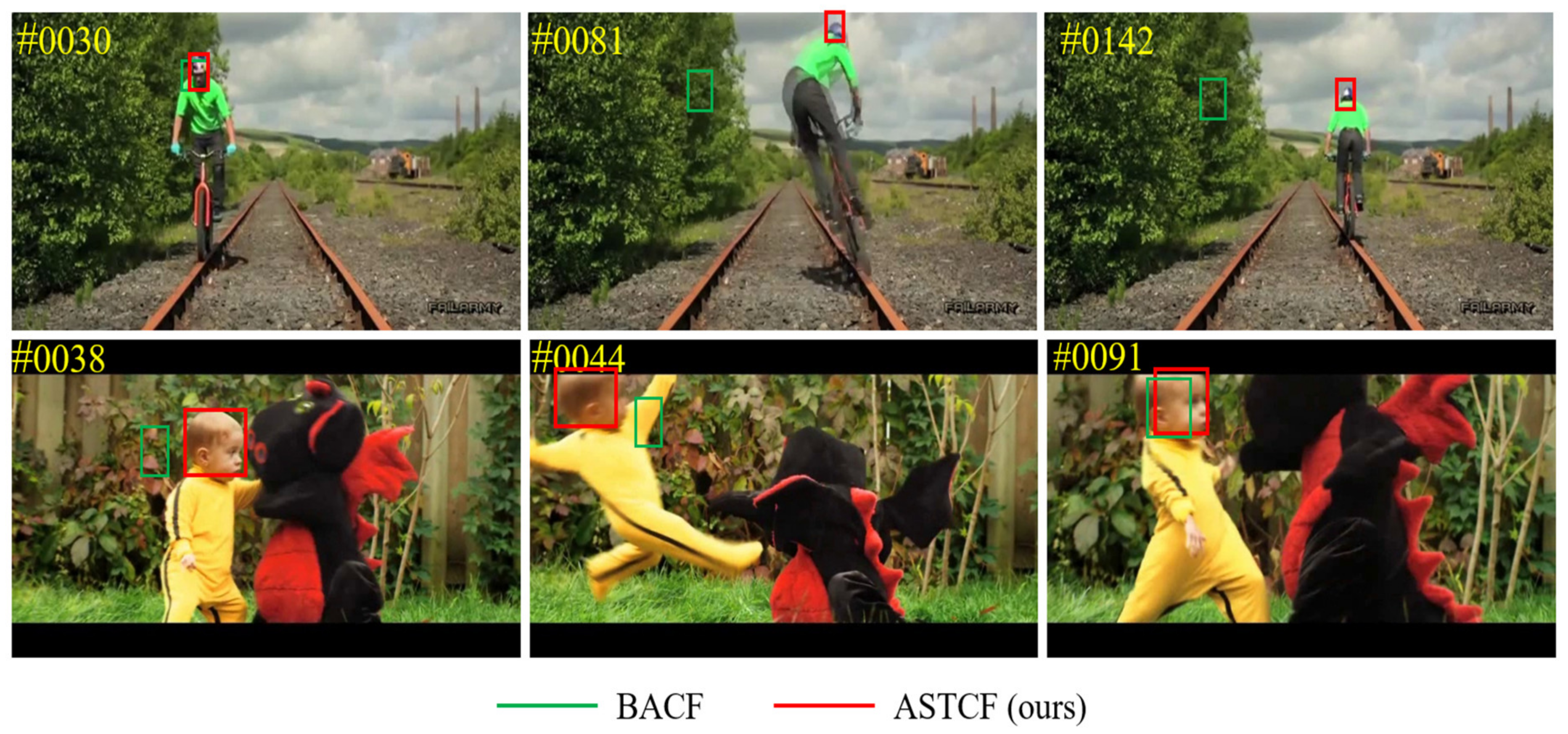
4.4. Qualitative Evaluation

To further verify the effectiveness of our tracking algorithm, we have taken the qualitative evaluations of eight trackers with the representative sequences, including Bird1, Skiing, Soccer, Coke, Freeman4, Singer2, and Ironman. There are seven compared trackers, including DeepSRDCF [33], ECO [42], MCPF [43], TADT [43], SimaFC [45], BACF [16], SRDCF [14]. Figure 8 shows the results of the qualitative evaluation. It can be seen that the proposed ASTCF method has achieved better tracking performance on qualitative evaluation, especially the tracking results after 100 frames. Take the Birds sequence for example, we can see that our ASTCF method can still track the object accurately after it disappears and reappears, but other trackers lose their tracked objects.

4.5. Temporal-Aware Constraint Parameter

The choice of temporal constraint parameter $\beta$ will influence the tracking performance, which is introduced in Equation (1) as the temporal-aware term.

Table 5. Precision and success rates on OTB2015 dataset with different temporal-aware regularization parameters $\beta$.

$\mathit{\beta }$	Precision	Success
10	0.871	0.662
11	0.879	0.669
12	0.887	0.672
13	0.895	0.681
14	0.919	0.689
15	0.918	0.692
16	0.927	0.699
17	0.920	0.689
18	0.912	0.680
19	0.901	0.682
20	0.896	0.677

shows the tracking performance when we choose different temporal regularization parameters. In this experiment, we present the value only from 10 to 20 at an interval of 1. It can be seen that the precision and success rates reached their highest values when we choose $\beta$ = 16.

4.6. Ablation Studies

This ablation study is to verify the effectiveness of the adaptive spatial regularization and temporal-aware terms of our ASTCF tracker; the results of different versions of ASTCF tracker on OTB2015 can be seen in

Table 6. DP scores and AUC scores of different versions of ASTCF on OTB2015 dataset.

Tracker	ASTCF	ASTCF-s	ASTCF-t	ASTCF-st
Precision (DP)	0.927	0.867	0.915	0.802
Success (AUC)	0.699	0.652	0.689	0.601

. ASTCF-s donates ASTCF without adaptive spatial regularization term, ASTCF-t donates ASTCF without temporal term and ASTCF-st donates ASTCF without adaptive spatial regularization and temporal-aware terms (equal baseline tracker). From the results of Table 6, we can see that the adaptive regularization and temporal-aware terms can effectively improve the performances of trackers, and they become better when fused together. Compared with ASTCF-s, ASTCF improves 6.0% in DP score and 4.7% in AUC score. Moreover, ASTCF also improves 1.2% in DP score and 1.0% in AUC score compared with ASTCF-t.

5. Conclusions

This paper proposes a novel adaptive spatial regularization and temporal-aware correlation filters (ASTCF) model for solving the unwanted boundary effects which occur in the correlation filters tracking. The proposed ASTCF method can help to build a robust appearance model and improve the tracking accuracy by introducing adaptive spatial regularization and temporal-aware terms into the objective function. Further, the objective function can be effectively optimized via the ADMM algorithm. The three related subproblems have analytical closed-form solutions, and greatly reduce the computational cost. Compared with other trackers on several benchmarks, the ASTCF method depicts obvious advantages on most of the evaluation metrics. For the OTB2015 dataset, our ASTCF tracker achieved the best results both on DP score and AUC score, which reached 0.699 and 0.927, respectively. Moreover, the speed of the ASTCF method is approximately 23.5 fps, which satisfies the requirements of real-time. In the future, we will further explore the application of this model for small object tracking on UAV and dark scenes.

References

1. Li, P.X.; Wang, D.; Wang, L.J.; Lu, H.C. Deep visual tracking: Review and experimental comparison. Pattern Recognit. 2018, 76, 323–338. [Google Scholar] [CrossRef]
2. Smeulders, A.W.; Chu, D.M.; Cucchiara, R.; Calderara, S.; Dehghan, A. Visual tracking: An experimental survey. IEEE Trans. Pattern Anal. Mach. Intell. 2014, 36, 1442–1468. [Google Scholar] [PubMed] [Green Version]
3. Wang, N.Y.; Shi, J.; Yeung, D.Y.; Jia, J. understanding and diagnosing visual tracking systems. In Proceedings of the IEEE International Conference on Computer Vision (ICCV), Santiago, Chile, 7–13 December 2015; pp. 3101–3109. [Google Scholar]
4. Yilmaz, A.; Javed, O.; Shah, M. Object tracking: A survey. ACM Comput. Surv. 2006, 38, 1–45. [Google Scholar] [CrossRef]
5. Sundararaman, R.; De Almeida Braga, C.; Marchand, E.; Pettré, J. Tracking Pedestrian Heads in Dense Crowd. In Proceedings of the 2021 IEEE/CVF Conference on Computer Vision and Pattern Recognition (CVPR), Virtual, 19–25 June 2021; pp. 3864–3874. [Google Scholar] [CrossRef]
6. Jang, J.; Jiang, H. MeanShift++: Extremely Fast Mode-Seeking with Applications to Segmentation and Object Tracking. In Proceedings of the 2021 IEEE/CVF Conference on Computer Vision and Pattern Recognition (CVPR), Virtual, 19–25 June 2021; pp. 4100–4111. [Google Scholar] [CrossRef]
7. Yu: Yu, Y.; Chen, L.; He, H.; Liu, J.; Zhang, W.; Xu, G. Second-Order Spatial-Temporal Correlation Filters for Visual Tracking. Mathematics 2022, 10, 684. [Google Scholar] [CrossRef]
8. Liu, L.; Cao, J. End-to-end learning interpolation for object tracking in low frame-rate video. IET Image Process. 2020, 14, 997–1216. [Google Scholar] [CrossRef]
9. Bolme, D.S.; Beveridge, J.R.; Draper, B.A.; Lui, Y.M. Visual object tracking using adaptive correlation filters. In Proceedings of the Twenty-Third IEEE Conference on Computer Vision and Pattern Recognition, CVPR 2010, San Francisco, CA, USA, 13–18 June 2010; pp. 2544–2550. [Google Scholar] [CrossRef]
10. Henriques, J.F.; Caseiro, R.; Martins, P.; Batista, J. Exploiting the Circulant Structure of Tracking-by-Detection with Kernels. In Computer Vision—ECCV; Springer: Berlin/Heidelberg, Germany, 2012; pp. 702–715. [Google Scholar]
11. Henriques, J.F.; Caseiro, R.; Martins, P.; Batista, J. High-Speed Tracking with Kernelized Correlation Filters. IEEE Trans. Pattern Anal. Mach. Intell. 2015, 37, 583–596. [Google Scholar] [CrossRef] [PubMed] [Green Version]
12. Liu, L.; Feng, T.; Fu, Y. Learning Multifeature Correlation Filter and Saliency Redetection for Long-Term Object Tracking. Symmetry 2022, 14, 911. [Google Scholar] [CrossRef]
13. Galoogahi, H.K.; Sim, T.; Lucey, S. Correlation Filters with Limited Boundaries. In Proceedings of the 2015 IEEE Conference on Computer Vision and Pattern Recognition (CVPR), Boston, MA, USA, 7–12 June 2015; pp. 4630–4638. [Google Scholar]
14. Danelljan, M.; Hager, G.; Khan, F.S.; Felsberg, M. Learning Spatially Regularized Correlation Filters for Visual Tracking. In Proceedings of the 2015 IEEE International Conference on Computer Vision (ICCV), Santiago, Chile, 7–13 December 2015; pp. 4310–4318. [Google Scholar] [CrossRef] [Green Version]
15. Danelljan, M.; Hager, G.; Khan, F.S.; Felsberg, M. Discriminative Scale Space Tracking. IEEE Trans. Pattern Anal. Mach. Intell. 2017, 39, 1561–1575. [Google Scholar] [CrossRef] [PubMed] [Green Version]
16. Galoogahi, H.K.; Fagg, A.; Lucey, S. Learning Background-Aware Correlation Filters for Visual Tracking. In Proceedings of the 2017 IEEE International Conference on Computer Vision (ICCV), Venice, Italy, 22–29 October 2017; pp. 1144–1152. [Google Scholar] [CrossRef] [Green Version]
17. Dai, K.; Wang, D.; Lu, H.; Sun, C.; Li, J. Visual Tracking via Adaptive Spatially-Regularized Correlation Filters. In Proceedings of the 2019 IEEE/CVF Conference on Computer Vision and Pattern Recognition (CVPR) 2019, Long Beach, CA, USA, 16–20 June 2019; pp. 4665–4674. [Google Scholar] [CrossRef]
18. Han, R.; Feng, W.; Wang, S. Fast Learning of Spatially Regularized and Content Aware Correlation Filter for Visual Tracking. IEEE Trans. Image Process. 2020, 29, 7128–7140. [Google Scholar] [CrossRef]
19. Danelljan, M.; Hager, G.; Khan, F.S.; Felsberg, M. Adaptive Decontamination of the Training Set: A Unified Formulation for Discriminative Visual Tracking. In Proceedings of the 2016 IEEE Conference on Computer Vision and Pattern Recognition (CVPR), Las Vegas, NV, USA, 27–30 June 2016; pp. 1430–1438. [Google Scholar] [CrossRef] [Green Version]
20. Li, F.; Tian, C.; Zuo, W.; Zhang, L.; Yang, M. Learning Spatial-Temporal Regularized Correlation Filters for Visual Tracking. In Proceedings of the 2018 IEEE/CVF Conference on Computer Vision and Pattern Recognition, Salt Lake City, UT, USA, 18–22 June 2018; pp. 4904–4913. [Google Scholar] [CrossRef] [Green Version]
21. Li, Y.; Fu, C.H.; Ding, F.Q.; Huang, Z.Y.; Lu, G. AutoTrack: Towards High-Performance Visual Tracking for UAV with Automatic Spatio-Temporal Regularization. In Proceedings of the 2020 IEEE/CVF Conference on Computer Vision and Pattern Recognition (CVPR), Virtual, 13–19 June 2020; pp. 11920–11929. [Google Scholar] [CrossRef]
22. Wu, Y.; Lim, J.; Yang, M. Object Tracking Benchmark. IEEE Trans. Pattern Anal. Mach. Intell. 2015, 37, 1834–1848. [Google Scholar] [CrossRef] [PubMed] [Green Version]
23. Matej, K.; Ales, L.; Jiri, M.; Michael, F.; Roman, P.; Luka, C.; Tomas, V.; Goutam, B.; Alan, L.; Abdelrahman, E.; et al. The Sixth Visual Object Tracking VOT2018 Challenge Results. In Computer Vision–ECCV 2018 Workshops. ECCV 2018. Lecture Notes in Computer Science; Leal-Taixé, L., Roth, S., Eds.; Springer: Cham, Switzerland, 2018; Volume 11129. [Google Scholar] [CrossRef]
24. Fan, H.; Lin, L.; Yang, F.; Chu, P.; Deng, G.; Yu, S.; Bai, H.; Xu, Y.; Liao, C.; Ling, H. LaSOT: A High-Quality Benchmark for Large-Scale Single Object Tracking. In Proceedings of the 2019 IEEE/CVF Conference on Computer Vision and Pattern RECOgnition (CVPR), Long Beach, CA, USA, 16–20 June 2019; pp. 5369–5378. [Google Scholar] [CrossRef] [Green Version]
25. Bertinetto, L.; Valmadre, J.; Golodetz, S.; Miksik, O.; Torr, P.H.S. Staple: Complementary Learners for Real-Time Tracking. In Proceedings of the 2016 IEEE Conference on Computer Vision and Pattern Recognition (CVPR), Las Vegas, NV, USA, 27–30 June 2016; pp. 1401–1409. [Google Scholar] [CrossRef] [Green Version]
26. Mueller, M.; Smith, N.; Ghanem, B. Context-aware correlation filter tracking. In Proceedings of the IEEE Conference on Computer Vision and Pattern Recognition (CVPR), Honolulu, HI, USA, 21–26 July 2017; pp. 1396–1404. [Google Scholar]
27. Ma, C.; Yang, X.; Zhang, C.Y.; Yang, M. Long-term correlation tracking. In Proceedings of the IEEE Conference on Computer Vision and Pattern Recognition (CVPR), Boston, MA, USA, 7–12 June 2015; pp. 5388–5396. [Google Scholar]
28. Tang, F.; Ling, Q. Contour-Aware Long-Term Tracking with Reliable Re-Detection. IEEE Trans. Circuits Syst. Video Technol. 2020, 30, 4739–4754. [Google Scholar] [CrossRef]
29. Wang, N.; Zhou, W.; Li, H. Reliable Re-Detection for Long-Term Tracking. IEEE Trans. Circuits Syst. Video Technol. 2019, 29, 730–743. [Google Scholar] [CrossRef]
30. Boyd, S. Distributed Optimization and Statistical Learning via the Alternating Direction Method of Multipliers. Found. Trends Mach. Learn. 2010, 3, 1–122. [Google Scholar] [CrossRef]
31. Wu, X.; Sahoo, D.; Hoi, S.C. Recent advances in deep learning for object detection. Neurocomputing 2020, 396, 39–64. [Google Scholar] [CrossRef] [Green Version]
32. Chen, J.; Zhou, M.; Huang, H.; Zhang, D.; Peng, Z. Automated extraction and evaluation of fracture trace maps from rock tunnel face images via deep learning. Int. J. Rock Mech. Min. Sci. 2021, 142, 104745. [Google Scholar] [CrossRef]
33. Danelljan, M.; Hager, G.; Khan, F.S.; Felsberg, M. Convolutional Features for Correlation Filter Based Visual Tracking. In Proceedings of the 2015 IEEE International Conference on Computer Vision Workshop (ICCVW), Santiago, Chile, 7–13 December 2015; pp. 621–629. [Google Scholar] [CrossRef] [Green Version]
34. Valmadre, J.; Bertinetto, L.; Henriques, J.; Vedaldi, A.; Torr, P.H.S. End-to-End Representation Learning for Correlation Filter Based Tracking. In Proceedings of the 2017 IEEE Conference on Computer Vision and Pattern Recognition (CVPR), Honolulu, HI, USA, 21–26 July 2017; pp. 5000–5008. [Google Scholar] [CrossRef] [Green Version]
35. Sun, Y.; Sun, C.; Wang, D.; He, Y.; Lu, H. ROI Pooled Correlation Filters for Visual Tracking. In Proceedings of the 2019 IEEE/CVF Conference on Computer Vision and Pattern Recognition (CVPR), Long Beach, CA, USA, 16–20 June 2019; pp. 5776–5784. [Google Scholar] [CrossRef]
36. Eckstein, J.; Bertsekas, D.P. On the Douglas—Rachford splitting method and the proximal point algorithm for maximal monotone operators. Math. Program. 1992, 55, 293–318. [Google Scholar] [CrossRef] [Green Version]
37. Karen, S.; Andrew, Z. Very deep convolutional networks for large-scale image recognition. arXiv 2014, arXiv:1409.1556. [Google Scholar]
38. Russakovsky, O.; Deng, J.; Su, H.; Krause, J.; Satheesh, S.; Ma, S.; Huang, Z.; Karpathy, A.; Khosla, A.; Bernstein, M.; et al. Imagenet large scale visual recognition challenge. Int. J. Comput. Vis. 2015, 115, 211–252. [Google Scholar] [CrossRef] [Green Version]
39. Wu, Y.; Lim, J.; Yang, M. Online Object Tracking: A Benchmark. In Proceedings of the 2013 IEEE Conference on Computer Vision and Pattern Recognition 2013, Portland, OR, USA, 23–28 June 2013; pp. 2411–2418. [Google Scholar] [CrossRef] [Green Version]
40. Li, B.; Wu, W.; Wang, Q.; Zhang, F.; Xing, J.; Yan, J. SiamRPN++: Evolution of Siamese Visual Tracking with Very Deep Networks. In Proceedings of the 2019 IEEE/CVF Conference on Computer Vision and Pattern Recognition (CVPR), Long Beach, CA, USA, 16–20 June 2019; pp. 4277–4286. [Google Scholar] [CrossRef] [Green Version]
41. Danelljan, M.; Robinson, A.; Shahbaz, K.F.; Felsberg, M. ECO: Efficient Convolution Operators for Tracking. In Proceedings of the 2017 IEEE Conference on Computer Vision and Pattern Recognition (CVPR), Honolulu, HI, USA, 21–26 July 2017; pp. 6931–6939. [Google Scholar] [CrossRef] [Green Version]
42. Zhang, T.; Xu, C.; Yang, M. Learning Multi-Task Correlation Particle Filters for Visual Tracking. IEEE Trans. Pattern Anal. Mach. Intell. 2019, 41, 365–378. [Google Scholar] [CrossRef] [PubMed]
43. Li, X.; Ma, C.; Wu, B.; He, Z.; Yang, M. Target-Aware Deep Tracking. In Proceedings of the 2019 IEEE/CVF Conference on Computer Vision and Pattern Recognition (CVPR), Long Beach, CA, USA, 16–20 June 2019; pp. 1369–1378. [Google Scholar] [CrossRef] [Green Version]
44. Nam, H.; Han, B. Learning Multi-domain Convolutional Neural Networks for Visual Tracking. In Proceedings of the 2016 IEEE Conference on Computer Vision and Pattern Recognition (CVPR), Las Vegas, NV, USA, 27–30 June 2016; pp. 4293–4302. [Google Scholar] [CrossRef] [Green Version]
45. Bertinetto, L.; Valmadre, J.; Henriques, J.F.; Vedaldi, A.; Torr, P.H.S. Fully-Convolutional Siamese Networks for Object Tracking. In Computer Vision–ECCV 2016 Workshops. ECCV 2016. Lecture Notes in Computer Science; Hua, G., Jégou, H., Eds.; Springer: Cham, Switzerland, 2016; Volume 9914. [Google Scholar] [CrossRef] [Green Version]
46. Song, Y.; Chao, M.; Wu, X.; Gong, L.; Yang, M. VITAL: Visual Tracking via Adversarial Learning. In Proceedings of the 2018 IEEE/CVF Conference on Computer Vision and Pattern Recognition, Salt Lake City, UT, USA, 18–22 June 2018; pp. 8990–8999. [Google Scholar] [CrossRef]
47. Zhang, Z.; Peng, H. Deeper and Wider Siamese Networks for Real-Time Visual Tracking. In Proceedings of the 2019 IEEE/CVF Conference on Computer Vision and Pattern Recognition (CVPR) Long Beach, CA, USA, 16–20 June 2019; pp. 4586–4595. [Google Scholar] [CrossRef] [Green Version]
48. Zhang, L.; Gonzalez-Garcia, A.; Weijer, J.V.D.; Danelljan, M.; Khan, F.S. Learning the Model Update for Siamese Trackers. In Proceedings of the 2019 IEEE/CVF International Conference on Computer Vision (ICCV), Seoul, Korea; 2019; pp. 4009–4018. [Google Scholar] [CrossRef] [Green Version]
49. Matej, K.; Jiri, M.; Alexs, L.; Tomas, V.; Roman, P.; Gustavo, F.; Georg, N.; Fatih, P.; Luka, C. A Novel Performance Evaluation Methodology for Single-Target Trackers. IEEE Trans. Pattern Anal. Mach. Intell. 2016, 38, 2137–2155. [Google Scholar] [CrossRef] [Green Version]
50. Choi, J.; Chang, H.J.; Fischer, T.; Yun, S.; Lee, K.; Jeong, J.; Demiris, Y.; Choi, J.Y. Context-Aware Deep Feature Compression for High-Speed Visual Tracking . In Proceedings of the 2018 IEEE/CVF Conference on Computer Vision and Pattern Recognition, Salt Lake City, UT, USA, 18–22 June 2018; pp. 479–488. [Google Scholar] [CrossRef]
Figure 1. The tracking results of ASTCF and BACF on two video sequences with motion blur and deformation.
Mathematics 10 04320 g001
Figure 2. The framework of adaptive spatial regularization and temporal-aware. Red bounding-boxes donate the final results.
Mathematics 10 04320 g002
Figure 3. Overall precision plots and success plots of OPE evaluated on OTB2015.
Mathematics 10 04320 g003
Figure 4. Precision plots of OPE on eleven video sequence attributions of OTB2015 dataset.
Mathematics 10 04320 g004
Figure 5. Success plots of OPE on eleven video sequence attributions of OTB2015.
Mathematics 10 04320 g005
Figure 6. Precision plots and success plots of OPE on LaSOT test dataset.
Mathematics 10 04320 g006
Figure 7. Success plots of OPE evaluate on fourteen sequence attributions.
Mathematics 10 04320 g007
Figure 8. Representative tracking results of qualitative evaluation. The selective sequences are Bird1, Skiing, Soccer, Coke, Freeman4, Singer2, and Ironman.
Mathematics 10 04320 g008