Design and Motion Characteristics of Active–Passive Composite Suspension Actuator

Abstract

The suspension system needs both an active mode and passive mode when the emergency rescue vehicle is running on a complex road. Therefore, an active–passive composite suspension actuator (APCSA) is designed in this paper. Firstly, combined with computational fluid dynamics theory and dynamic mesh technology, the complete fluid domain of the original passive suspension actuator (PSA) is simulated. Secondly, in accordance with the simulation results and in consideration of the working conditions of the active suspension of the emergency rescue vehicle, the APCSA is designed, and its flow field characteristics are studied. Finally, test results show that the maximum recovery damping force/compression damping force of the APCSA is 2428.98 N/−1470.29 N, which is 53.5%/50.4% lower than that of the original PSA. Hence, the dynamic response capability of the actuator is effectively improved, which lays a foundation for improving the ride comfort and handling stability of emergency rescue vehicles on complex roads.

1. Introduction

Emergency rescue vehicles are mainly used for rescues on land, which has a large load capacity and complex road conditions [1,2,3,4]. The suspension system can cushion the impact transmitted from the road to the vehicle body and ensure the driving smoothness and handling stability of the vehicle [5,6,7]. The commonly used suspension types include passive suspension, semiactive suspension and active suspension [8,9]. Compared with passive suspension and semiactive suspension, active suspension can actively adjust the suspension stiffness and damping parameters in accordance with the driving road conditions to improve the driving smoothness and stability of the vehicle [10,11,12]. In the case of ensuring the vibration suppression effect when driving on different roads, a single suspension mode cannot maintain low power consumption. Therefore, the suspension adopts an active mode under off-road conditions and a passive mode under good road conditions. This can effectively improve the environmental adaptability of the emergency rescue vehicle, reduce the power consumption and improve the operational life. A schematic of active and passive mode switching is shown in Figure 1. When the suspension is in the passive mode, the rod and rodless cavities of the actuator are connected with the accumulators to form a hydro-pneumatic spring. When the suspension is in the active mode, the rod and rodless cavities of the actuator are connected with a servo valve, and the servo valve controls the actuator to realize various control algorithms. The accumulator in front of the servo valve is used to stabilize the pressure pulsation, and the pump is driven by the engine. Furthermore, an overflow valve is set at the pump port to regulate the system pressure.

Mode switching is realized by a mode switching valve block.

A suspension actuator is a key component of active suspension. The performance of the actuator directly affects the performance of the active suspension, further affecting the ride comfort and handling stability of the whole vehicle [13,14,15]. The suspension actuator of existing emergency rescue vehicles is designed for passive suspension, which cannot satisfy the requirements of active mode and passive mode at the same time. Therefore, it is necessary to design an active–passive composite suspension actuator (APCSA) to meet the needs of switching between active mode and passive mode. The channel parameters of the rod and rodless cavities in the suspension actuator will affect the actuator movement. If a channel’s diameter is too small, it will increase the accumulation of pressure loss, reduce the circuit efficiency and cause noise and vibration [16,17]. Therefore, the design of the channels is particularly important.

Computational fluid dynamics (CFD) combines numerical calculation methods with data visualization to simulate the flow of liquid. It is a new technical method to solve the flow problem, in addition to theoretical analysis and experimental measurement [18,19,20]. Dynamic mesh technology can be used to simulate the problem wherein the flow field shape changes with time [21,22,23,24,25].

Abdalla et al. [26] used the Fluent software to study the influence of the actuator outlet size on flow and piston speed, and the simulation results showed that increasing the outlet area can increase the actuator flow and piston speed. Behrens et al. [27] used dynamic mesh technology to simulate the dynamic characteristics of a high-frequency actuator under the influences of inertia and oil compressibility. Lai et al. [28] used the CFD model to study the pressure characteristics of a hydraulic cylinder and found that the CFD model showed a better pattern of cushion processing compared with other models. Li et al. [29] analyzed the interior flow field in different clearance conditions and at different rotation rates in a rotary hydraulic cylinder with Fluent. The existing literature has simplified the fluid domain of an actuator, neglected the structure of the flow channel and reduced the accuracy of the simulation.

In this study, in consideration of the complex road conditions of emergency rescue vehicles, two suspension working modes are designed. Combined with CFD theory and dynamic mesh technology, the complete fluid domain of a passive suspension actuator (PSA) is simulated. Then, the actuator structure is redesigned to improve the motion characteristics of the actuator, making it an APCSA that considers the needs of active and passive modes. Lastly, the performance of the APCSA is tested by experiments.

2. Numerical Simulation of Flow Field

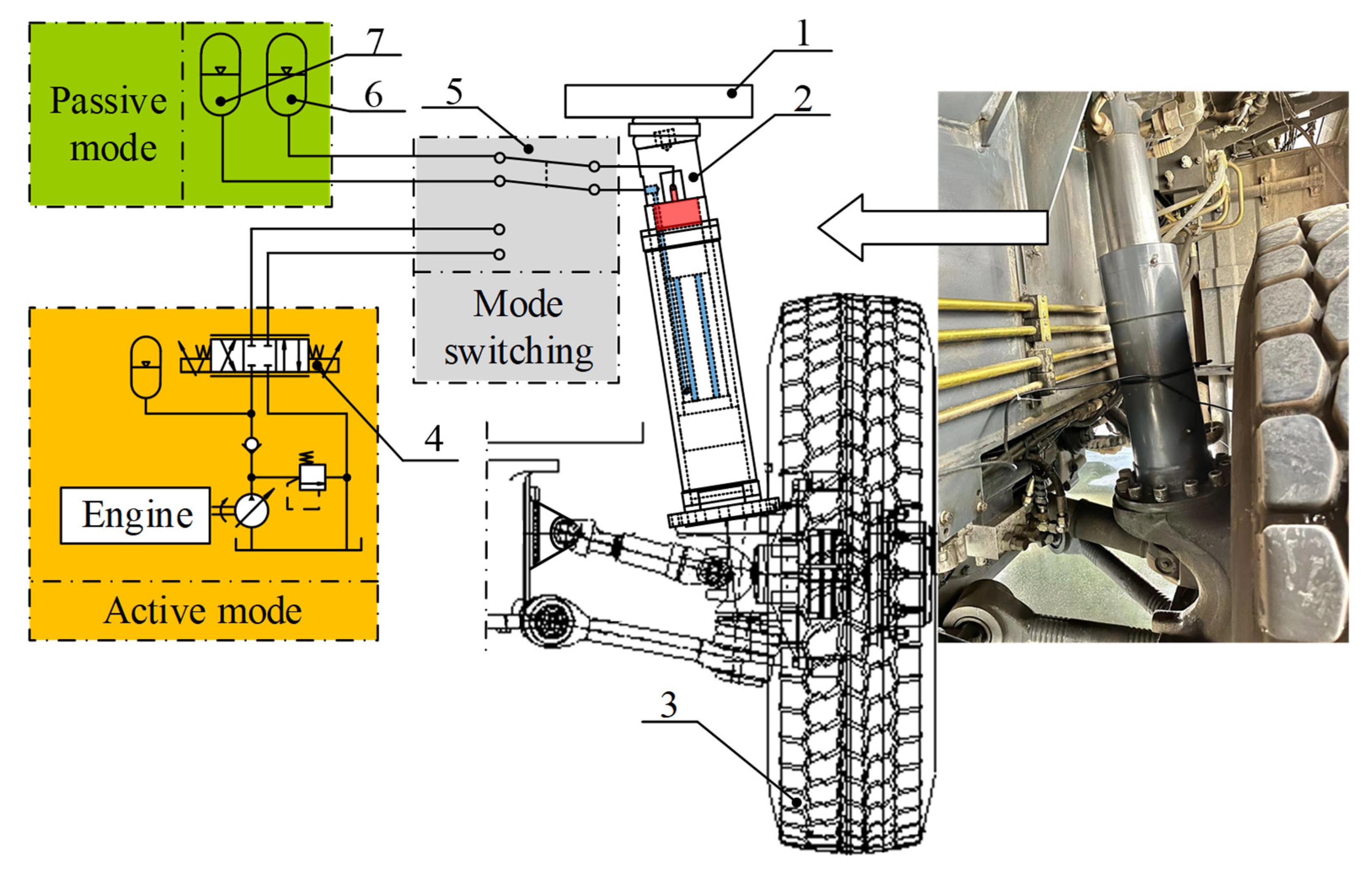
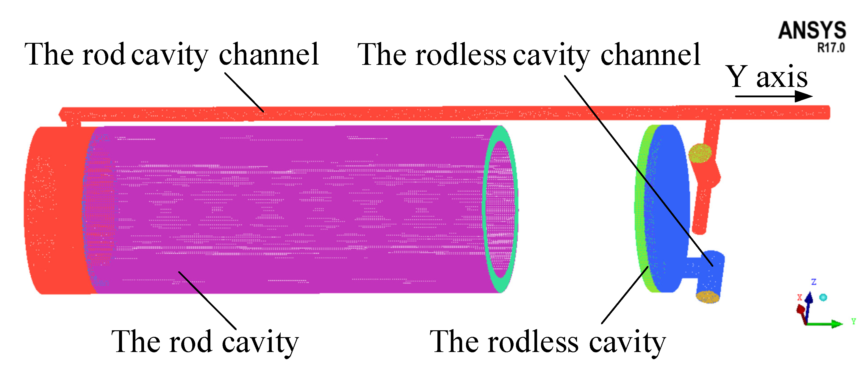
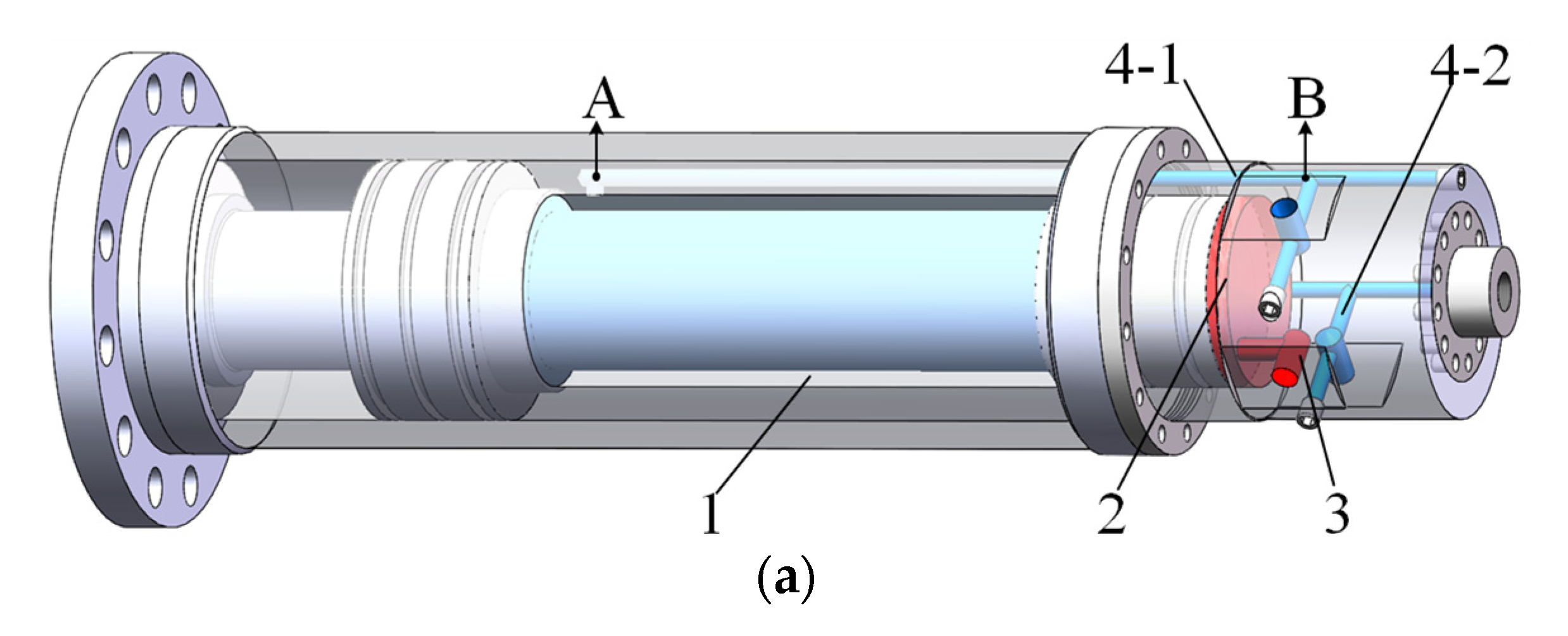
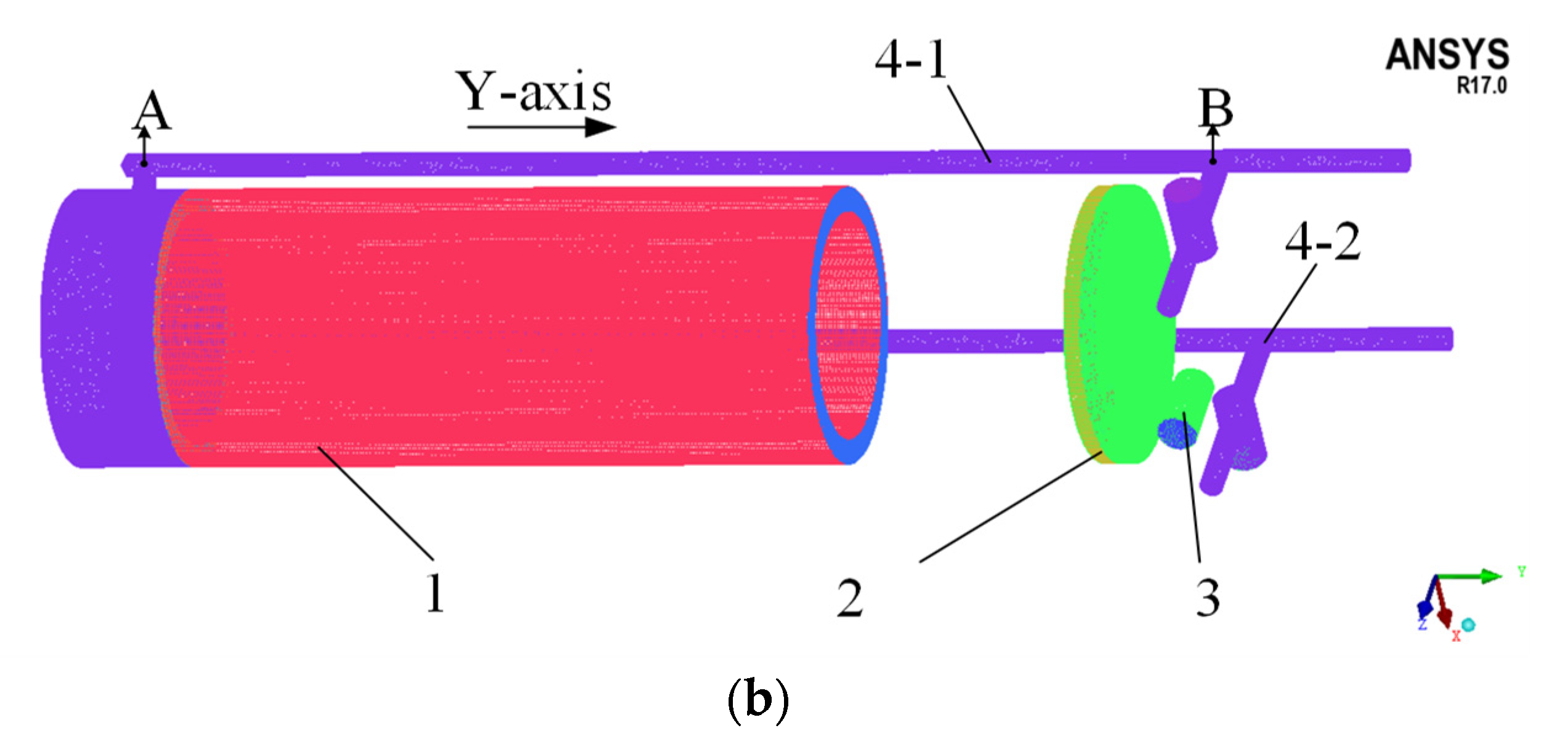
2.1. Actuator Structure and Geometric Modelling

The PSA of an emergency rescue vehicle is taken as the research object. The structural model is shown in Figure 2. The diameter of the rodless cavity is 80 mm, the diameter of the rodless cavity channel is 10 mm, the diameter of the piston rod is 70 mm, the diameter of the rod cavity channel is 8 mm, and the stroke is 200 mm. The fluid domain is composed of four parts: the rod cavity, the rodless cavity, the rod cavity channel and the rodless cavity channel. The dynamic mesh technology is used to simulate the movement process of the piston rod, which lays the foundation for the structural design of the APCSA.

The diameter of the hoses connecting the actuator and other components is 20 mm, which is much larger than the diameter of the internal flow channel of the actuator. Therefore, the flow resistance of the hoses can be ignored.

2.2. Flow Field Simulation

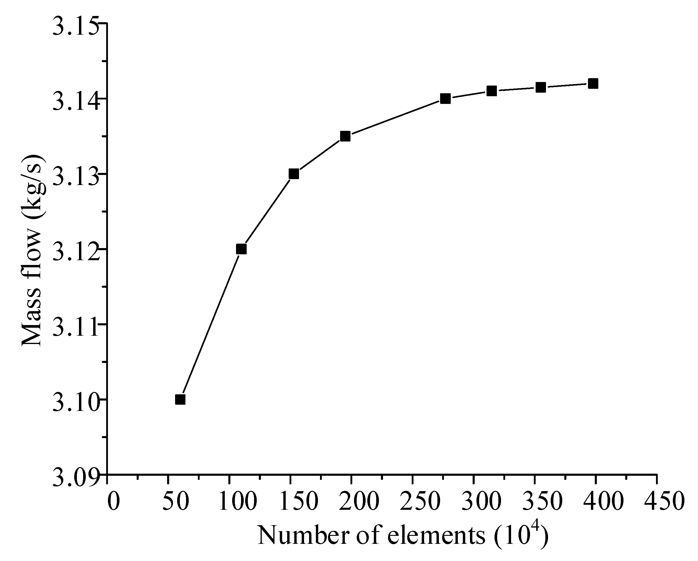
2.2.1. Meshing

To improve the mesh quality, the fluid domain model is imported into ICEM CFD for mesh generation. Since the shape of the piston motion area is regular, it is divided into hexahedral meshes. Furthermore, since the shapes of the channels are irregular, they are divided into tetrahedral meshes. Given the small size of the channel, a boundary layer effect exists in the flow, so the boundary layer grid is denser to ensure the effectiveness of the simulation results. Before the final determination of the mesh model, the mesh independence is verified to ensure that the final calculation results are the least sensitive to the change in mesh density. Taking the mass flow at the outlet as an indicator, the calculation result is as shown in Figure 3.

It can be seen from Figure 3 that when the number of elements exceeds 2.7 million, the mass flow at the outlet tends to be stable. In order to reduce the amount of computation and obtain reliable results, the total number of grids is determined to be approximately 2.7 million.

The fluid domain mesh model is shown in Figure 4. This study completely retains the real model of the actuator fluid domain and does not simplify it, such as via the intersection of flow channels, to ensure the correctness of the simulation results.

2.2.2. Fluid Mechanical Governing Equation

The following equations are applied.

The continuity equation is

$$\frac{\partial \rho }{\partial t}+\mathrm{div}(\overrightarrow{u})=\frac{\partial \rho }{\partial t}+\frac{\partial \left(\rho u_1\right)}{\partial x}+\frac{\partial \left(\rho u_2\right)}{\partial y}+\frac{\partial \left(\rho u_3\right)}{\partial z}=0.$$

(1)

The momentum equation is

$$\{\begin{array}{l}\frac{\partial (\rho u_1)}{\partial t}+\mathrm{div}(\rho \overrightarrow{u}{u}_1)=\mathrm{div}(\mu \mathrm{g}\mathrm{r}\mathrm{a}\mathrm{d}{u}_1)-\frac{\partial p}{\partial x}+S_1\\ \frac{\partial (\rho u_2)}{\partial t}+\mathrm{div}(\rho \overrightarrow{u}{u}_2)=\mathrm{div}(\mu \mathrm{g}\mathrm{r}\mathrm{a}\mathrm{d}{u}_2)-\frac{\partial p}{\partial y}+S_2\\ \frac{\partial (\rho u_3)}{\partial t}+\mathrm{div}(\rho \overrightarrow{u}{u}_3)=\mathrm{div}(\mu \mathrm{g}\mathrm{r}\mathrm{a}\mathrm{d}{u}_3)-\frac{\partial p}{\partial z}+S_3\end{array}$$

(2)

The energy conservation equation is

$$\frac{\partial \left(\rho T\right)}{\partial t}+\frac{\partial \left(\rho u_{1}T\right)}{\partial x}+\frac{\partial \left(\rho u_{2}T\right)}{\partial y}+\frac{\partial \left(\rho u_{3}T\right)}{\partial z}=\frac{\partial }{\partial x}\left(\frac{k_p}{c_p}\frac{\partial T}{\partial x}\right)+\frac{\partial }{\partial y}\left(\frac{k_p}{c_p}\frac{\partial T}{\partial y}\right)+\frac{\partial }{\partial z}\left(\frac{k_p}{c_p}\frac{\partial T}{\partial z}\right)+S_T$$

(3)

The transport equations of turbulent kinetic energy k and dissipation rate ε are

$$\frac{\partial (\rho k)}{\partial t}+\frac{\partial (\rho k{u}_i)}{\partial x_i}=\frac{\partial }{\partial x_j}\left[\left(\mu +\frac{{\mu }_t}{{\sigma }_k}\right)\frac{\partial k}{\partial x_j}\right]+G_k-\rho \epsilon +S_k,$$

(4)

$$\frac{\partial (\rho \epsilon )}{\partial t}+\frac{\partial (\rho \epsilon u_i)}{\partial x_i}=\frac{\partial }{\partial x_j}\left[\left(\mu +\frac{{\mu }_t}{{\sigma }_k}\right)\frac{\partial \epsilon }{\partial x_j}\right]+C_{1\epsilon }\frac{\epsilon }{k}{G}_k-C_{2\epsilon }\rho \frac{{\epsilon }^2}{k}+S_{\epsilon }.$$

(5)

where ρ is the density of fluid. u_i and u_j are the velocity components of fluid in three directions (i = 1, 2, 3; j = 1, 2, 3); that is, u₁, u₂ and u₃ are the velocity components of fluid in the x, y and z directions, respectively. S_i is the generalized source term, (I = 1, 2, 3). p is the pressure on the fluid element. k_p is the heat transfer coefficient of the fluid. c_p is the specific heat capacity. T is the temperature. S_T is the part of the fluid mechanical energy converted into heat energy. μ is the dynamic viscosity. μ_t is the turbulent viscosity. k is the turbulence kinetic energy. G_k is the turbulent kinetic energy generation term caused by the average velocity gradient. σ_k and σ_ε are the Prandtl numbers corresponding to k and ε, respectively. S_k and S_ε are user-defined source terms. C_1ε and C_2ε are empirical constants; that is, C_1ε = 1.44, C_2ε = 1.92, σ_k = 1.0, and σ_ε = 1.3.

2.2.3. Parameter Setting

ANSYS Fluent is used for the numerical simulation of the model. The turbulence model is set as standard k–ε. The hydraulic oil is ISO-L-HM46 with a density of 889 kg /m³ and a dynamic viscosity of 0.04048 Pa·s. The inlet of the rodless cavity is set as the ‘Pressure Inlet’, and the pressure is 1.5 MPa. The outlet of the rod cavity is set as the ‘Pressure Outlet’, and the pressure is 0.05 MPa. The solver is set as ‘Pressure-Based’, and the calculation method is ‘SIMPLE’.

The strategy of dynamic mesh updating adopts the ‘Layering’ updating method. The movement of the piston in the dynamic domain is defined by ‘DEFINE_ CG_ MOTION’, and the piston movement speed is set to 0.3 m/s. As the stroke of the actuator is relatively short, which is ±0.1 m, when the speed is 0.3 m/s, it only takes 0.33 s for the actuator to reach the maximum stroke. Therefore, the speed is reasonable for the practical operation of suspension in off-road conditions.

3. Simulation Results and Analysis

The flow speed and pressure loss of oil can be determined by analyzing the flow field inside the suspension actuator, which can provide a theoretical reference for the structural design of the actuator. Given that the motion speed of the actuator is 0.3 m/s, four simulation time points within 0.67 s are selected to analyze the dynamic flow field characteristics of the suspension actuator during its extension movement.

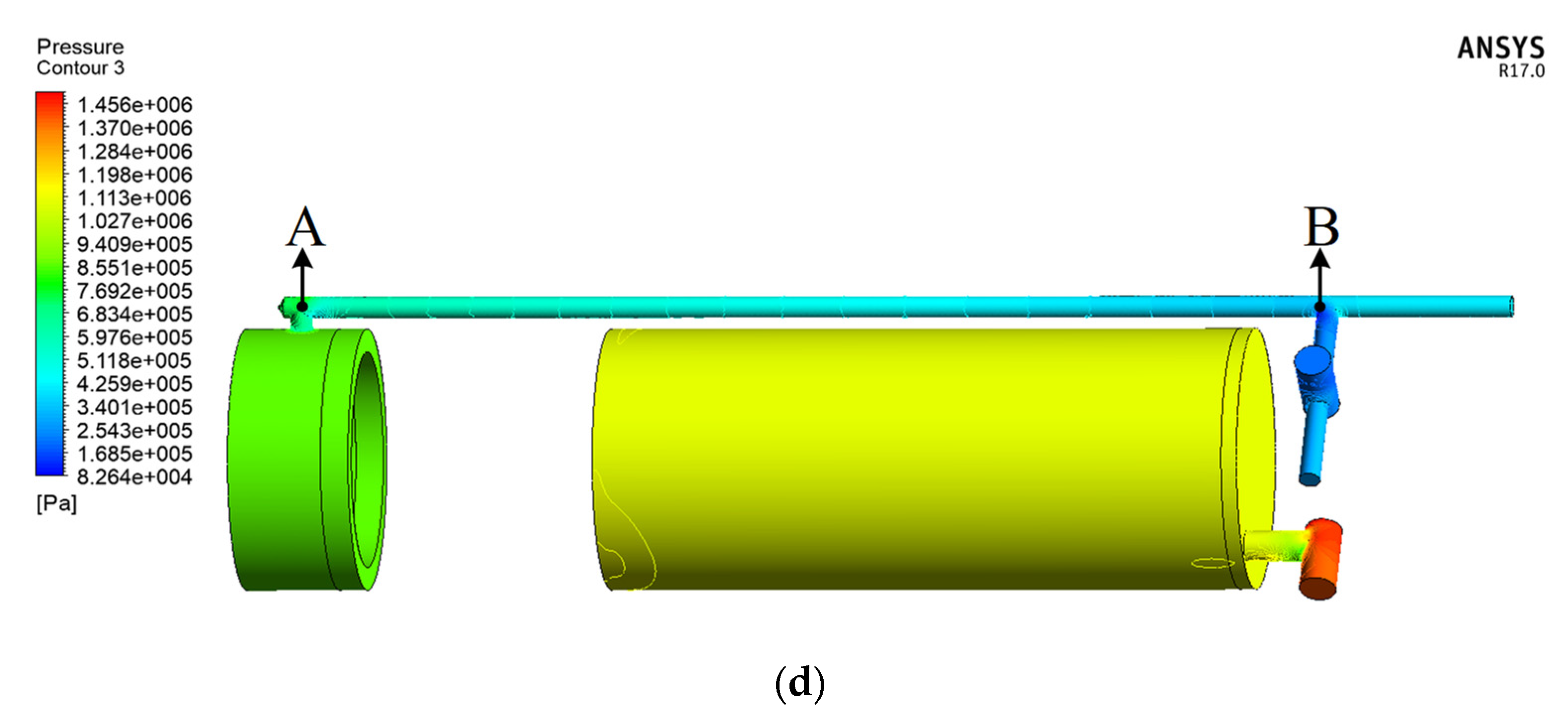
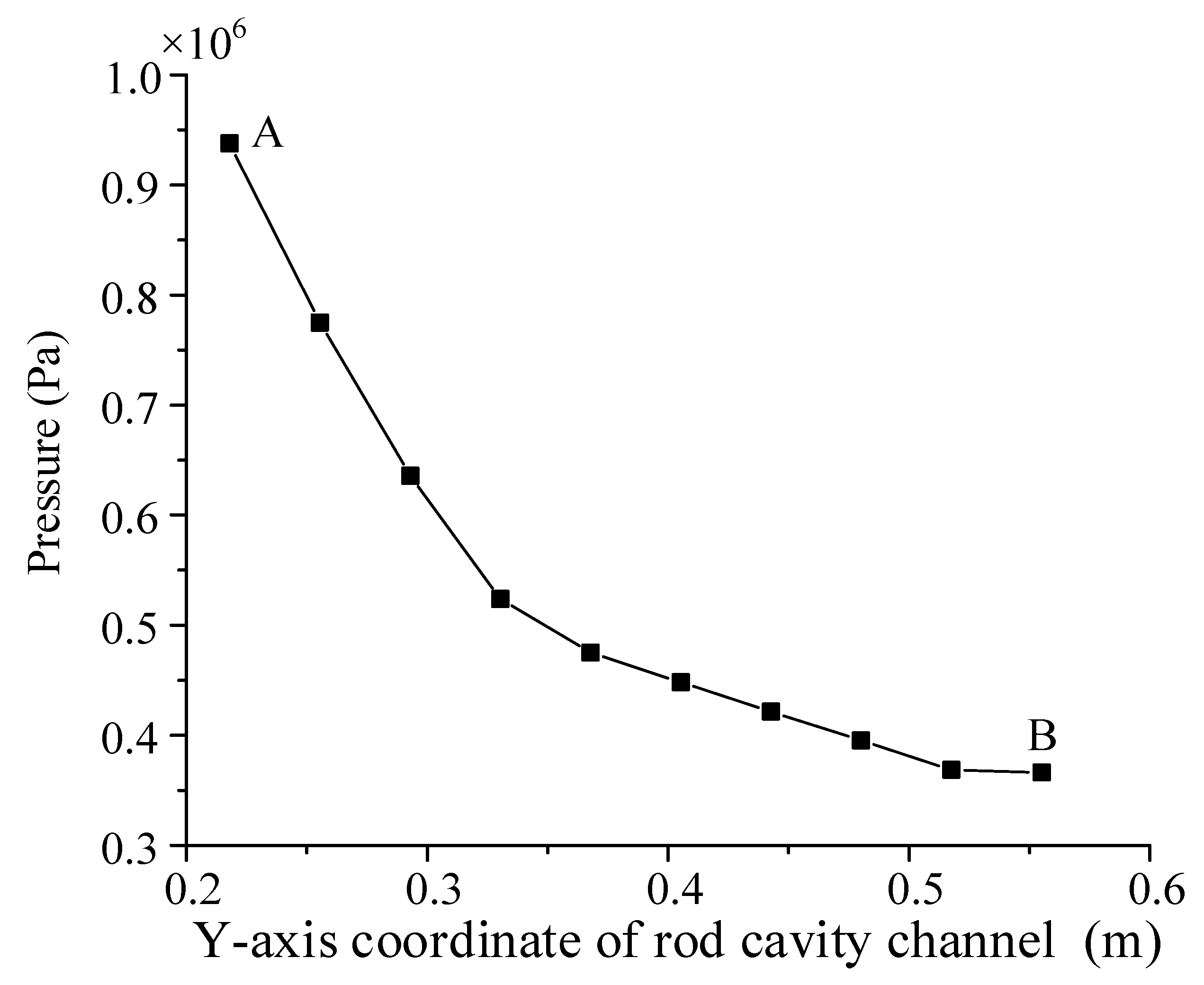
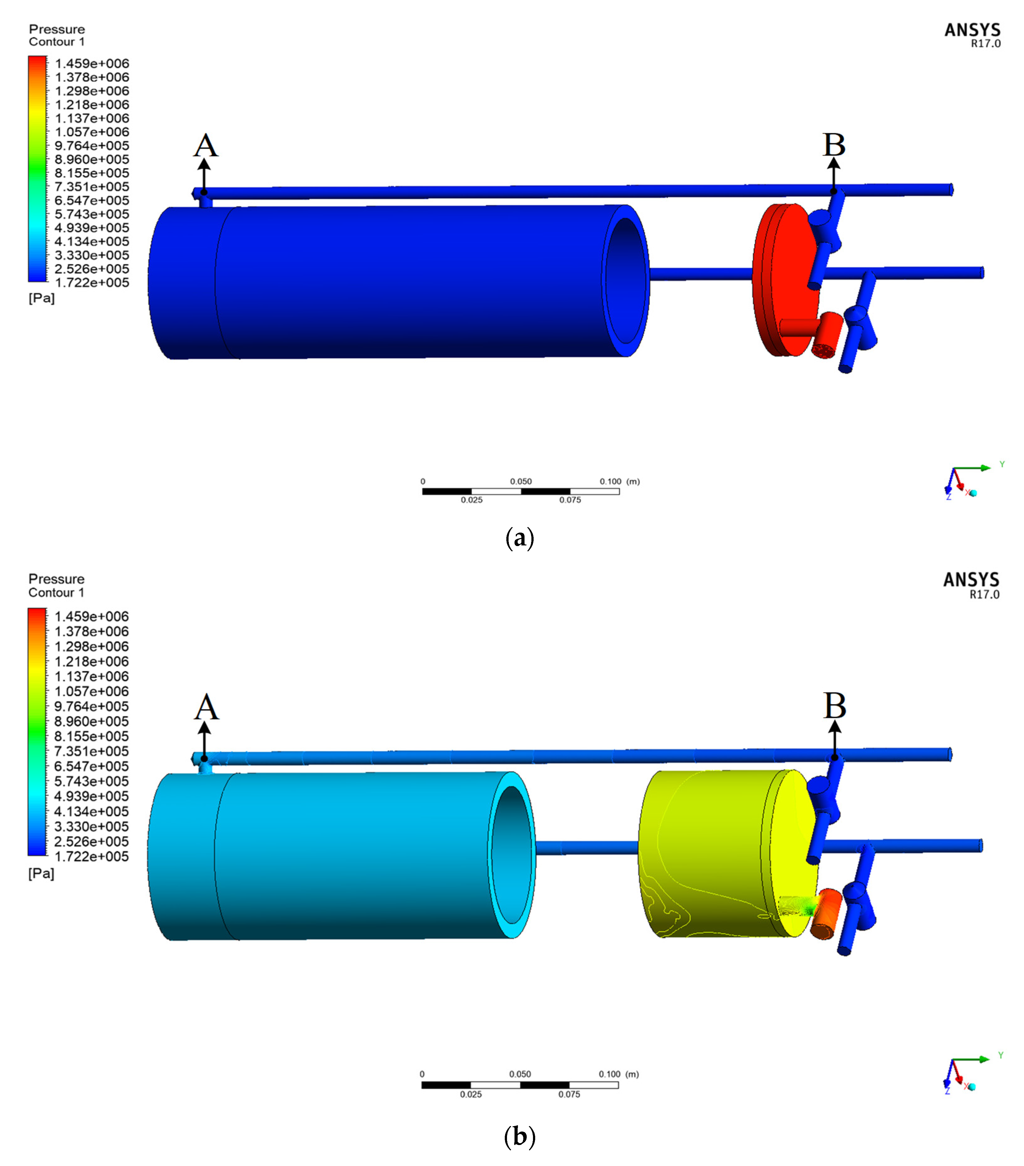
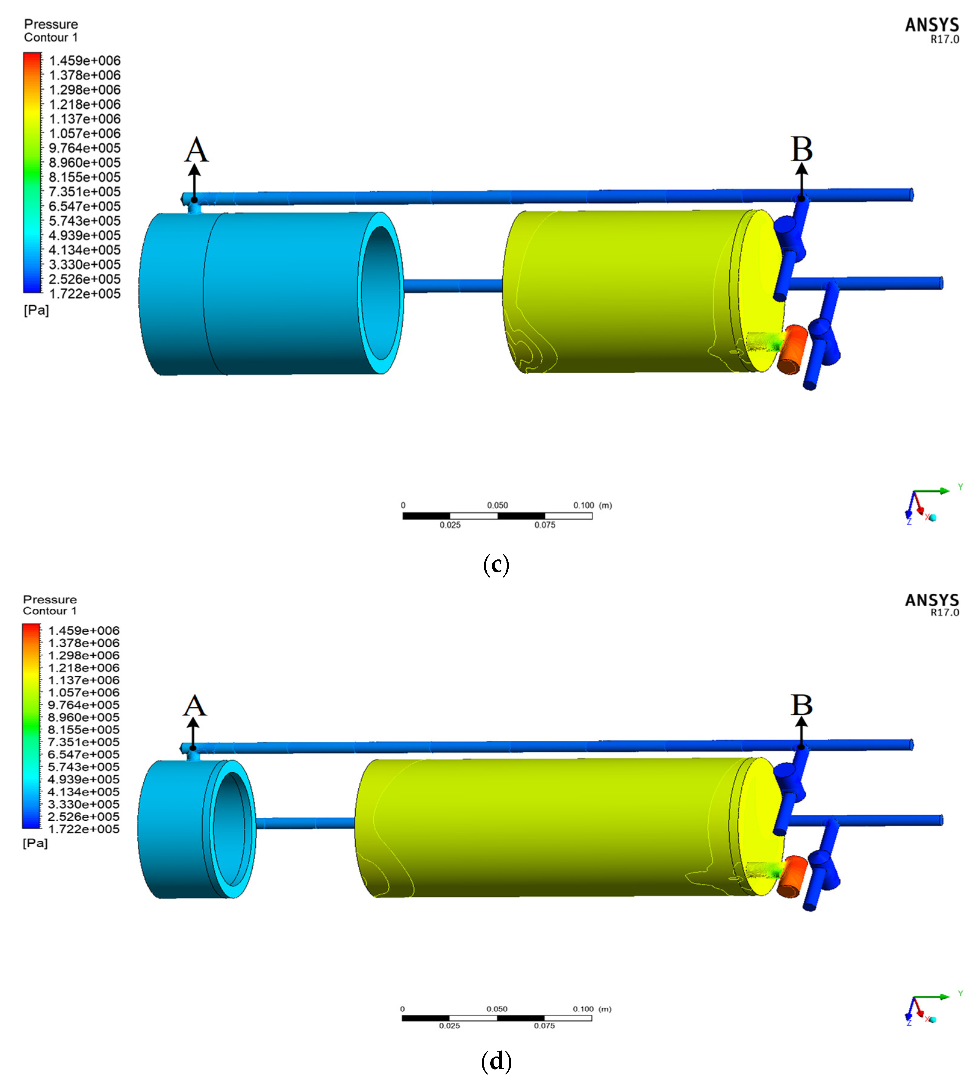
3.1. Actuator Flow Field Pressure Contour

The pressure contour of the actuator flow field is shown in Figure 5.

Figure 5 illustrates that during the extension movement of the actuator, a large pressure drop occurs from point A to point B in the rod cavity channel. When t = 0.67 s, the pressure from point A to point B at 10 positions is taken. The pressure curve is shown in Figure 6. The pressure of point A is 0.938 MPa and that of point B is 0.366 MPa, and the pressure loss is 0.572 MPa. Because the small diameter of the rod cavity channel causes a large pressure loss, the rod cavity channel needs to be redesigned.

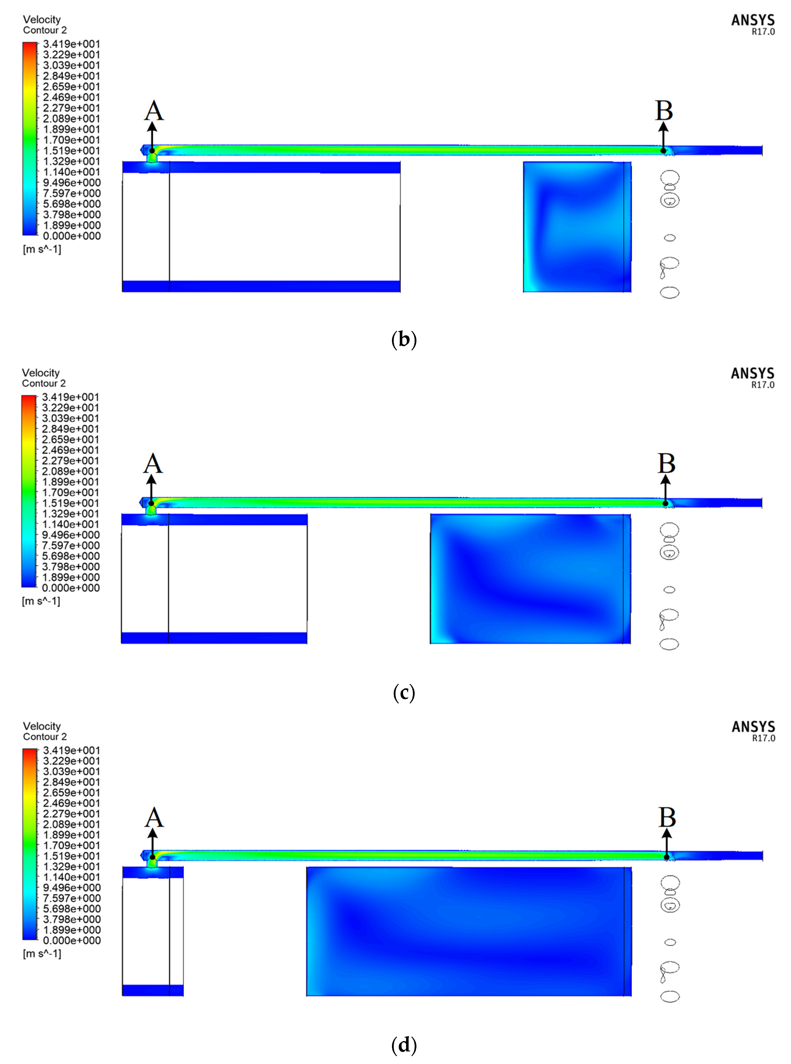
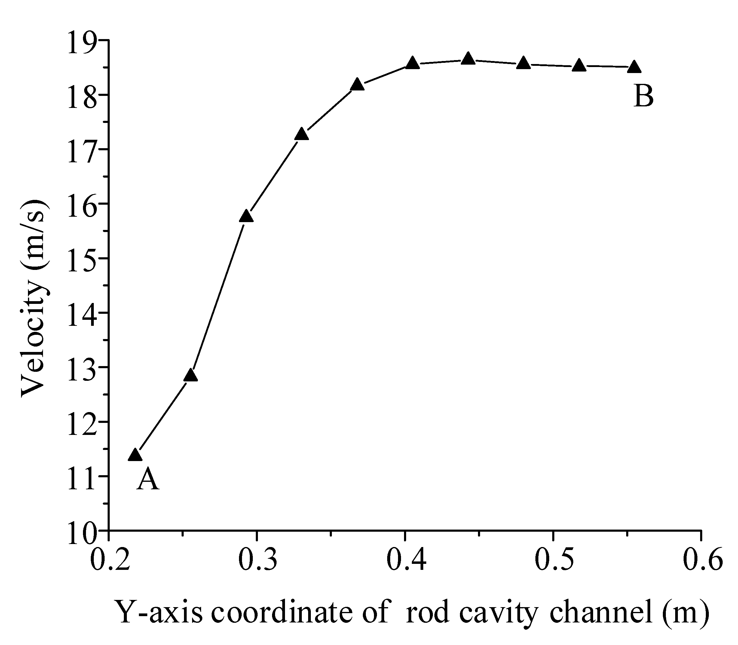
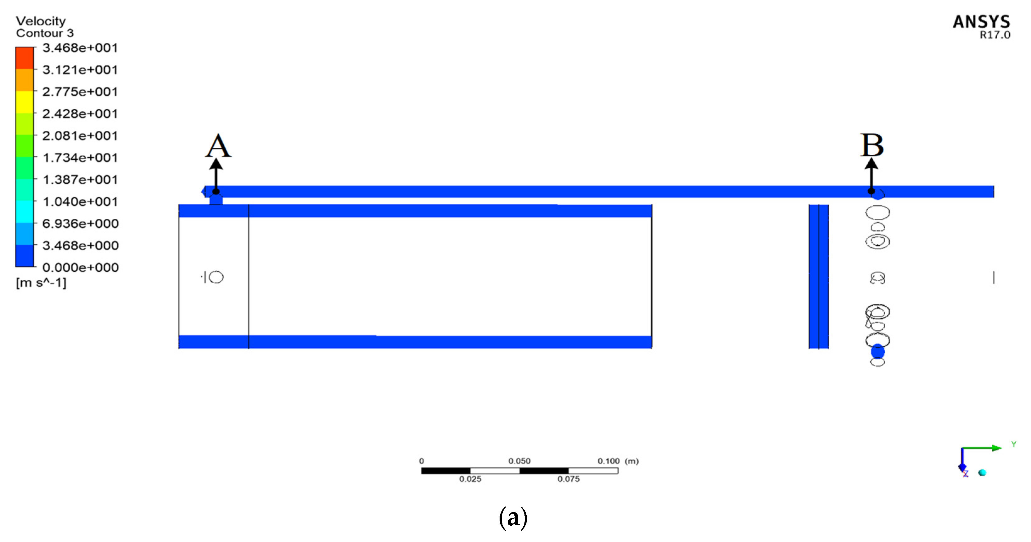
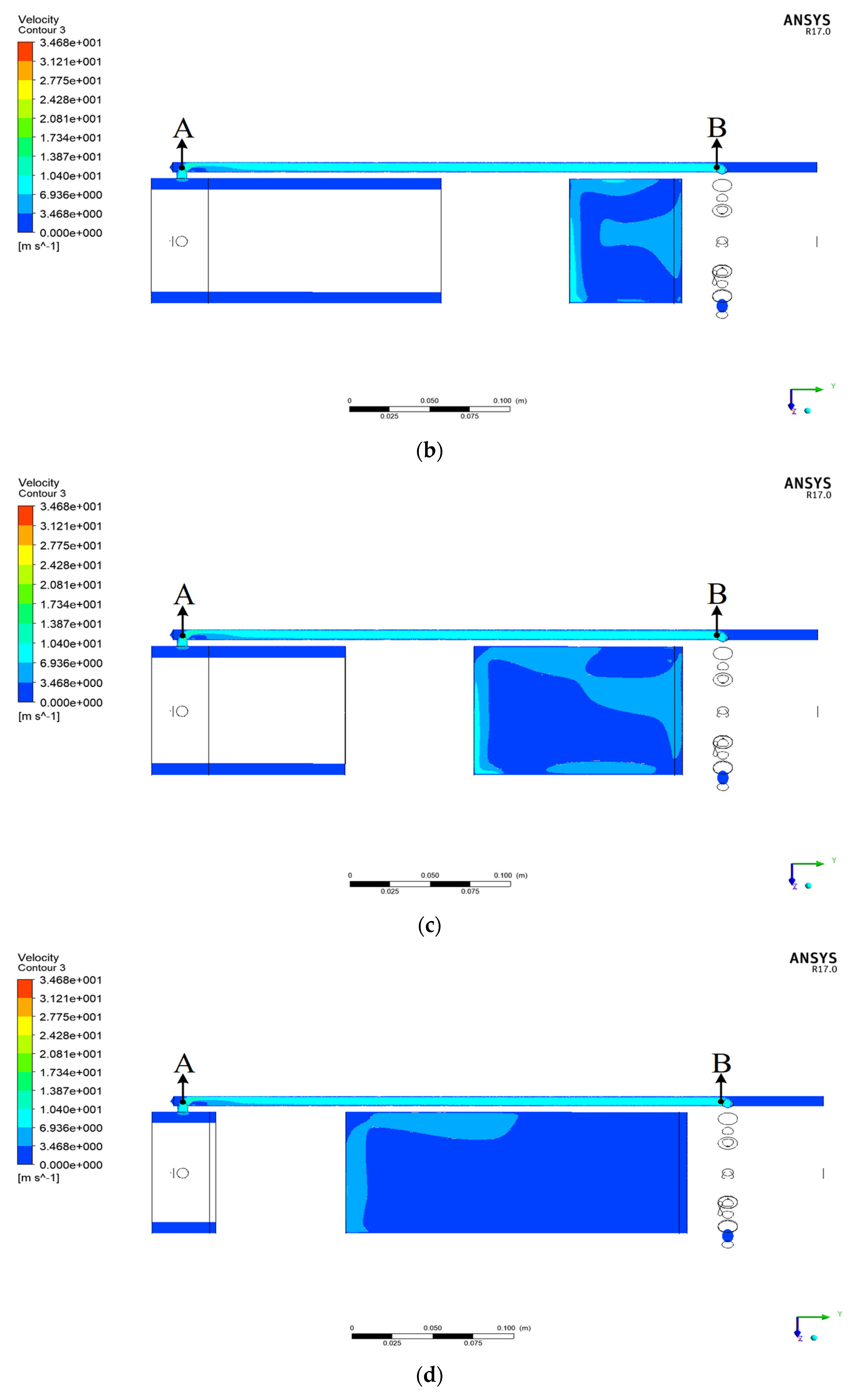
3.2. Actuator Flow Field Velocity Contour

The velocity contour of the actuator flow field is shown in Figure 7.

As seen in Figure 7, during the extension movement of the actuator, the flow speed of the oil increases after it enters the rod cavity channel from the rod cavity, whilst the speed of other parts, such as the rodless cavity, does not change significantly. The flow speed from point A to point B at 10 positions at t = 0.67 s is determined. The velocity curve is shown in Figure 8. The maximum flow speed from point A to point B is 18.63 m/s, and the flow speed at most locations is stable near this velocity. Therefore, during the extension movement of the actuator, the flow speed of the rod cavity channel is too fast to be achieved in the experiment, so the rod cavity channel should be redesigned to reduce the flow speed.

4. Structure Design and Flow Field Simulation of the APCSA

4.1. Structural Design of the APCSA

Given that the installation position of the suspension actuator on an emergency rescue vehicle is difficult to change, the external dimensions of the APCSA should be the same as before. To improve the motion characteristics and responsiveness of the actuator in active mode, a rod cavity channel 4-2 (Figure 9) is added, which enlarges the equivalent flow area of the rod cavity channel. During the movement of the actuator, the two rod cavity channels work together to improve the flow capacity of the rod cavity. On the premise of guaranteeing the structural strength and not changing the installation size, the diameter d of flow channel 4-2 is set to 5 mm, 6 mm, 7 mm and 8 mm. The smaller flow passage diameter can allow the actuator to obtain better structural strength. Therefore, if the smaller channel diameter can meet the requirements of flow speed and pressure drop, the smaller diameter will be selected. Therefore, the selection of the channel diameter is the result of considering the structural strength, pressure drop and flow rate.

The simulation parameters are consistent with those presented in Section 2.2.3. Dynamic mesh simulation is carried out in Fluent.

When t = 0.67 s, the pressure and flow velocity at 10 positions from point A to point B in rod cavity channel 4-1 are taken, and the comparison curves are as shown in Figure 10 and Figure 11.

As seen in Figure 10 and Figure 11, the larger the diameter of rod cavity channel 4-2, the smaller the pressure and pressure drop from point A to point B, and the lower the steady flow speed between points A and B. A comparison of the pressure drops from point A to point B with different diameters is shown in Figure 12, and a comparison of the steady flow speeds is displayed in Figure 13.

Figure 12 and Figure 13 demonstrate that when the diameter d of rod cavity 4-2 is 5 mm, 6 mm, 7 mm and 8 mm, respectively, the pressure drop from point A to point B decreases by 29.7%, 43.2%, 62.1% and 75.7%, respectively, compared with PSA, and the steady flow speed between points A and B decreases by 31.0%, 41.6%, 47.8% and 56.0%, respectively. Therefore, on the premise of ensuring the structural strength and not changing the installation size, the diameter d of rod cavity channel 4-2 should preferably be 8 mm.

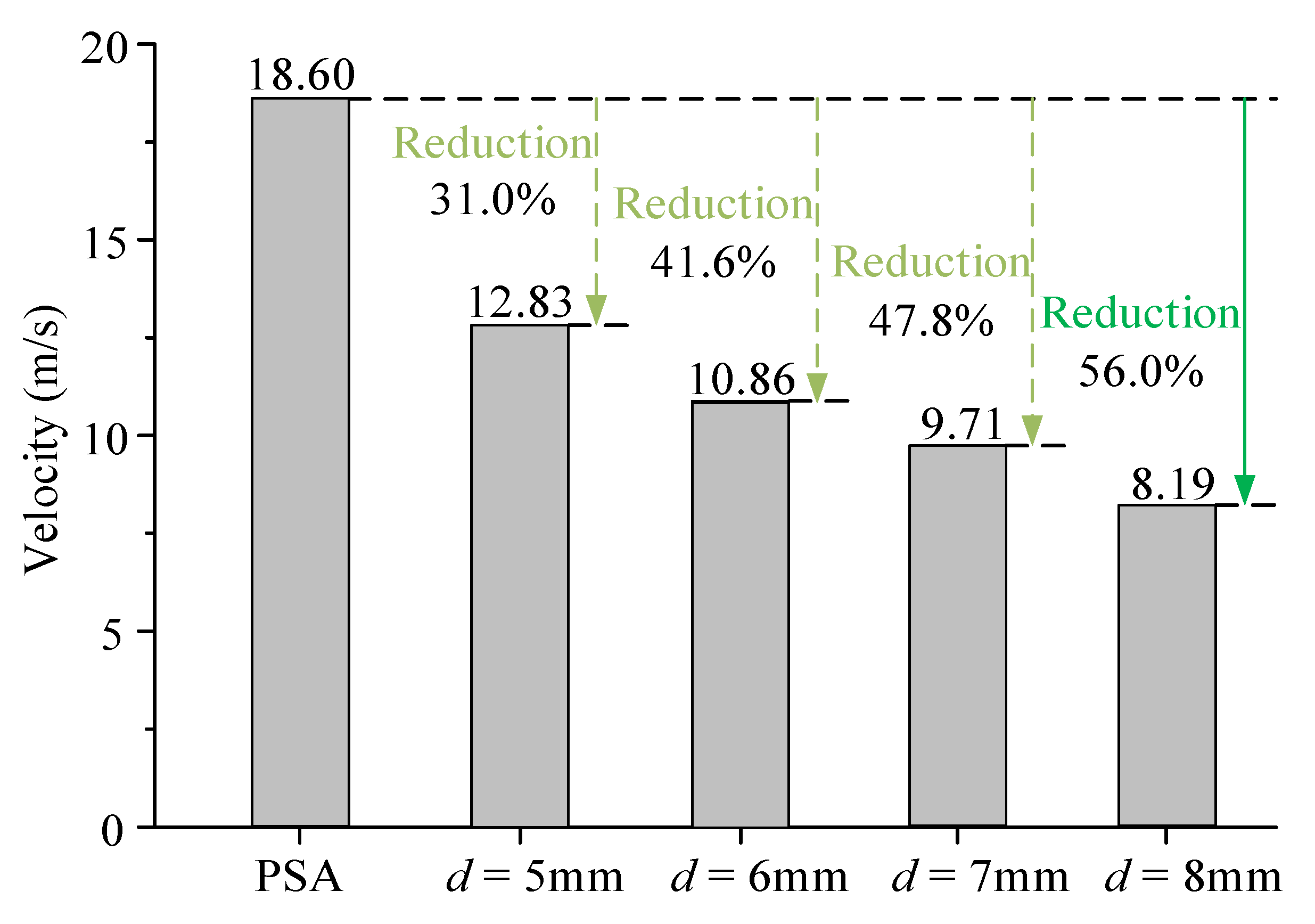
4.2. Simulation Results (d = 8 mm)

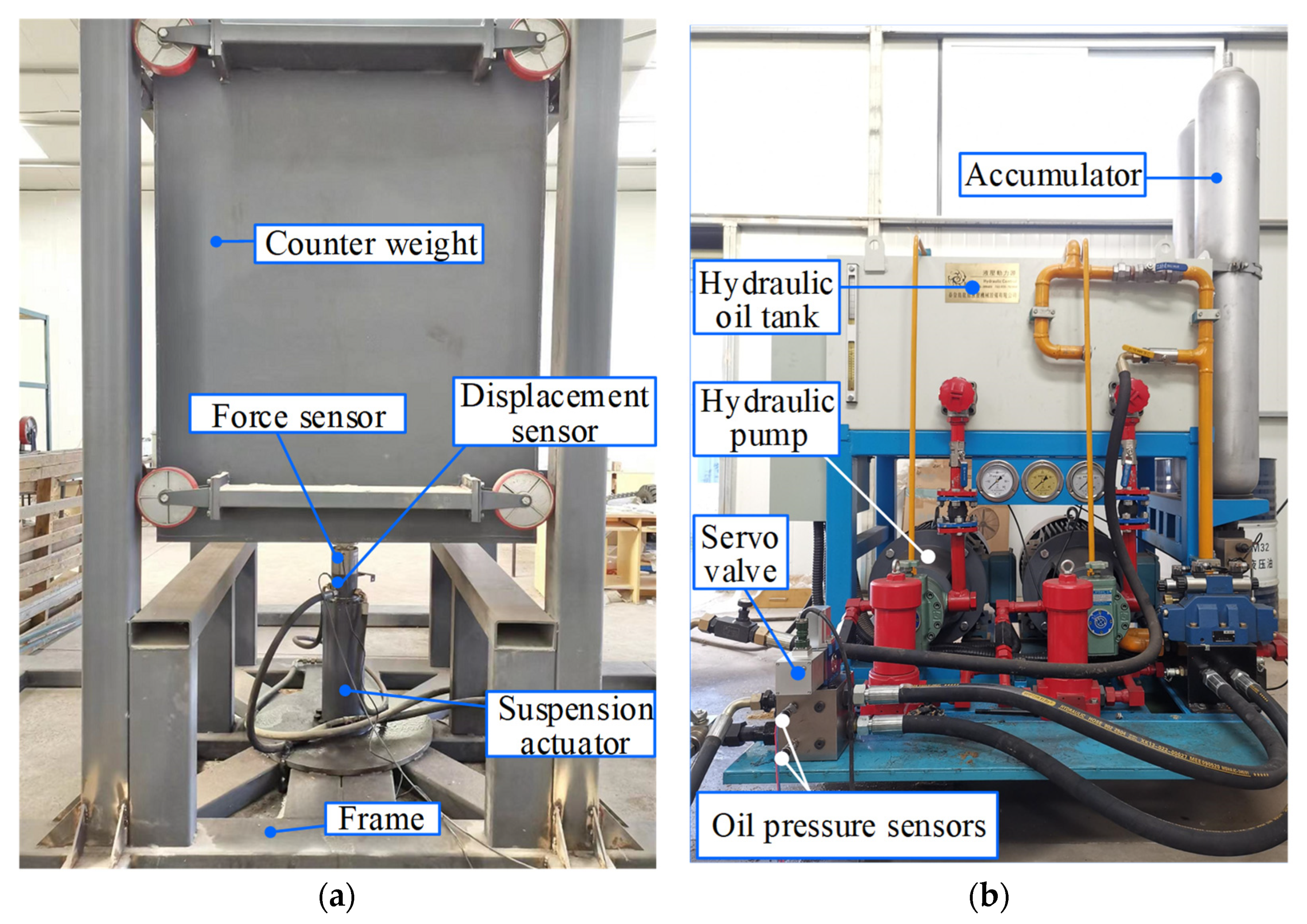
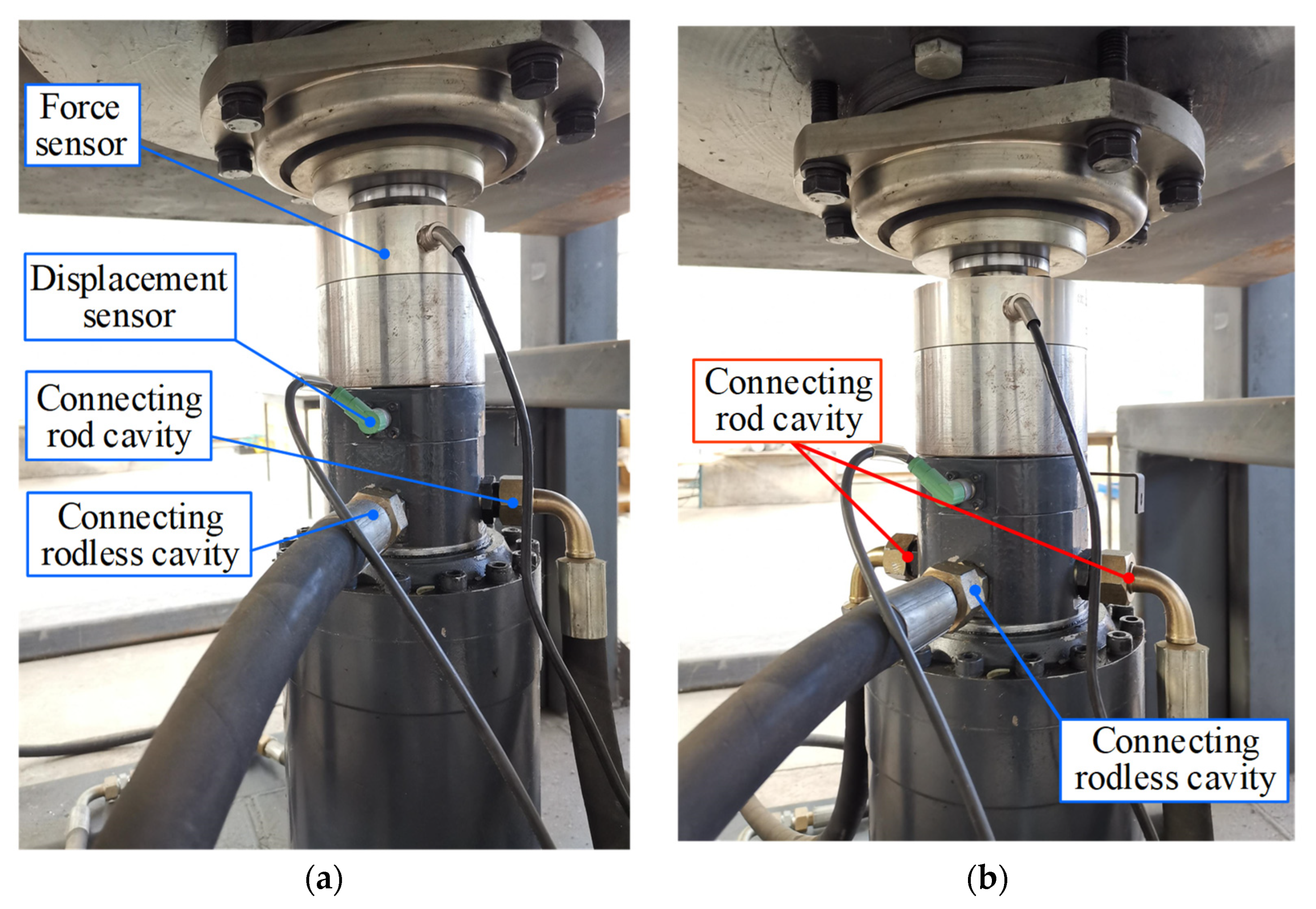
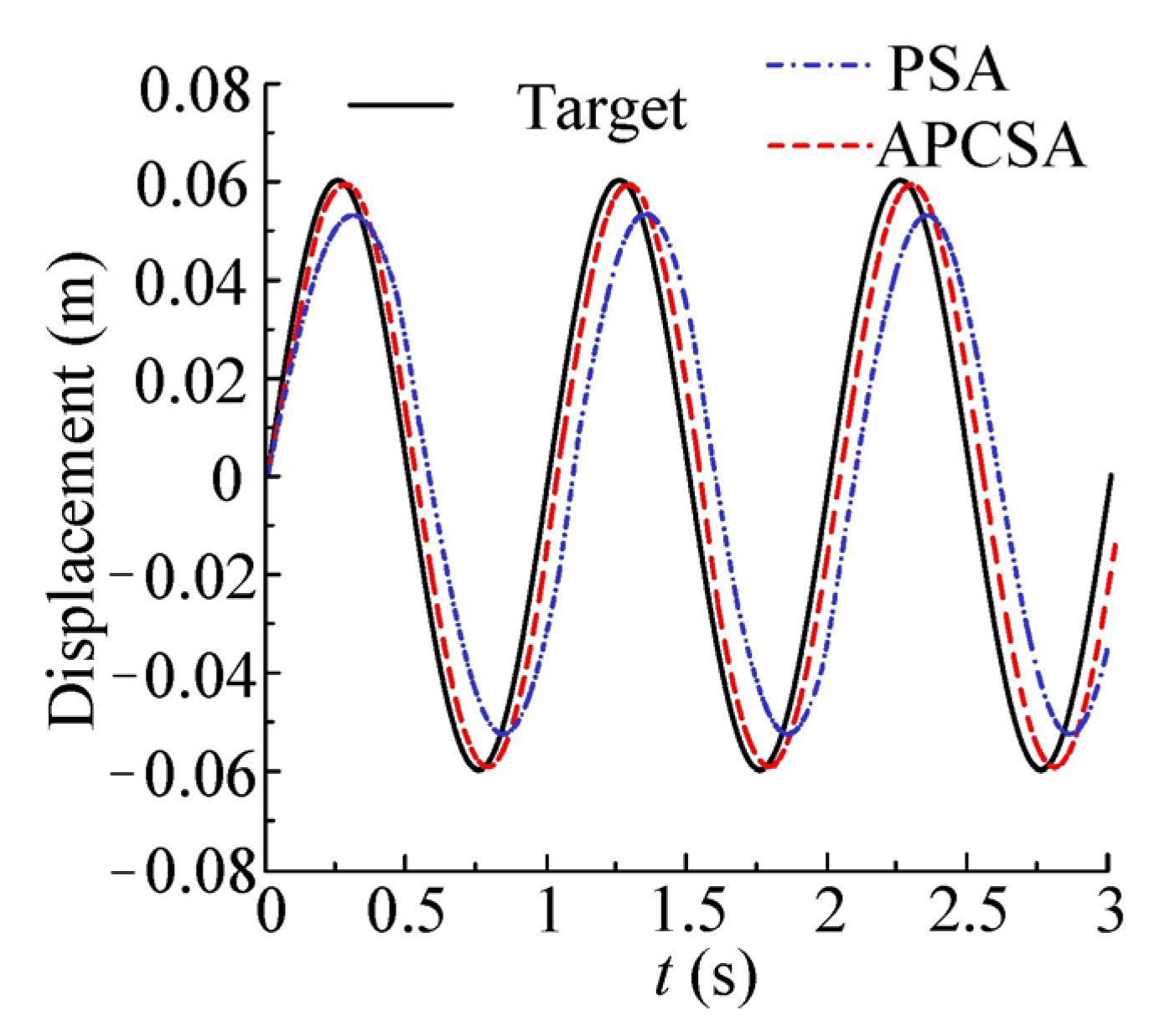
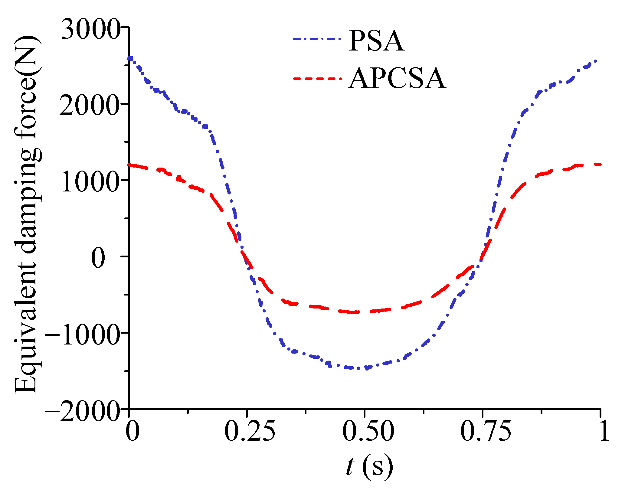
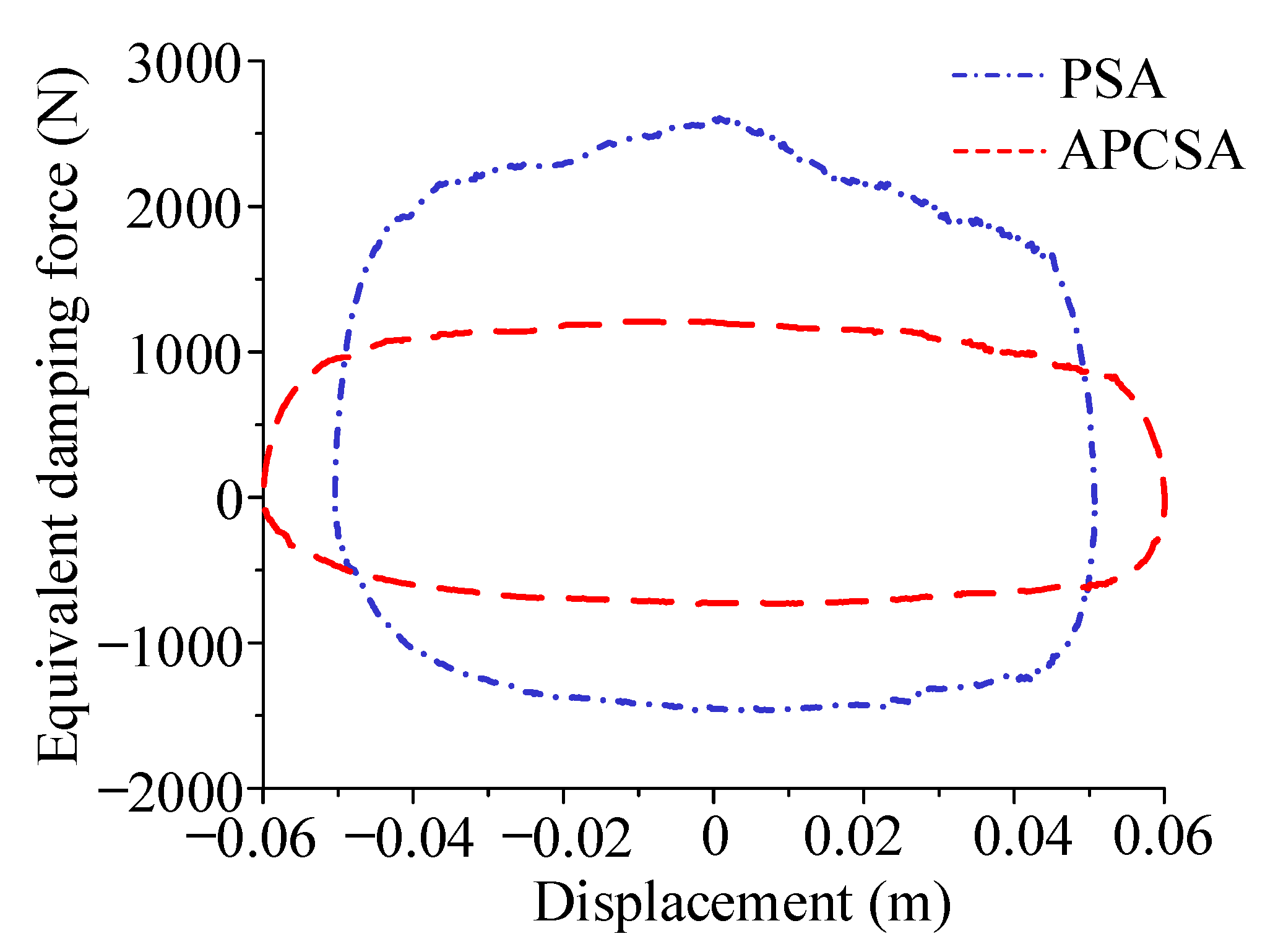
The flow field pressure contour of the APCSA when the diameter of rod cavity channel 4-2 is 8 mm is shown in Figure 14. Given the symmetrical structure of the two rod cavity channels, taking rod cavity channel 4-1 as an example, the flow field velocity contour diagram of its profile is as shown in Figure 15.

Figure 14 demonstrates that during the extension movement of the actuator—that is, when t = 0.2 s, t = 0.4 s and t = 0.67 s—the pressure drop from point A to point B in the rod cavity channel is small. As seen in Figure 10, when t = 0.67 s, the pressure at point A is 0.387 MPa, and the pressure at point B is 0.248 MPa, so the pressure drop is 0.139 MPa. Compared with PSA, the APCSA effectively reduces the pressure loss in the rod cavity channel.

As seen in Figure 15, during the extension movement of the actuator, the flow speed of the oil increases after it enters the rod cavity channel from the rod cavity, whilst the speed of other parts, such as the rodless cavity, does not change significantly. Figure 11 illustrates that the maximum flow velocity from point A to point B is 8.19 m/s, and the flow velocity at most positions is stable around this velocity. Compared with PSA, the APCSA effectively reduces the flow velocity in the rod cavity channel and meets the requirements of the actuator movement speed.

5. Experiment

To further compare the performance of the PSA and APCSA, a suspension actuator test bench is established, as shown in Figure 16. The APCSA test bench is divided into an actuating bench and a pumping station. The actuating bench includes a counterweight, a force sensor, a suspension actuator and a frame, etc. The pumping station includes an electro-hydraulic servo valve, an oil pressure sensor, a hydraulic pump, a hydraulic oil tank and an accumulator, etc. The PSA is shown in Figure 17a, and the APCSA is shown in Figure 17b. In the experiment, the diameter of rod cavity channel 4-2 is 8 mm, and the mass of the counterweight is 1000 kg. In addition, the pressure at the pump outlet is 9 MPa.

A displacement step and square wave response tests are carried out for the PSA and APCSA, respectively. The actuator structure is the only variable, and other conditions, such as system pressure and counterweight weight, remain the same. The experimental response curves are shown in Figure 18 and Figure 19.

Figure 18 shows that under the step signal, the time required for the PSA to rise to 0.06 m is 0.284 s, and the time required for the APCSA is 0.193 s, which is 32% less than the rising time of the PSA; in other words, the response speed of the APCSA is significantly improved.

As seen in Figure 19, under the square wave signal, the response time of the APCSA during rising and falling decreases. A comparison diagram of the mean values for rising to 0.06 m three times is shown in Figure 19b. The mean time of the PSA rising to 0.06 m is 0.262 s, and the mean time of the APCSA rising is 0.182 s, which is 30.5% lower than that of the PSA. Therefore, the response speed of the APCSA is proven to be significantly improved once again.

Sinusoidal signals with an amplitude of 0.06 m and frequencies of 0.5 and 1 Hz are used to test the following effect of the two actuators. The displacement curves of the experimental results are shown in Figure 20 and Figure 21.

The time delay and amplitude attenuation ratio are used as performance indexes, and a comparison is shown in

Table 1. Performance index comparison.

Comparison	Time Delay (s)		Amplitude Attenuation Ratio (%)
	0.5 Hz	1 Hz	0.5 Hz	1 Hz
PSA	0.10	0.13	5.5	10.8
APCSA	0.04	0.05	0.3	0.5
Performance improvement	60.0%	61.5%	94.5%	95.4%

. Figure 20 and Table 1 indicate that under the sinusoidal signal with a frequency of 0.5 Hz, the time delay of the displacement curve of the PSA is 0.10 s, and the amplitude attenuation ratio is 5.5%. The time delay of the APCSA is 0.04 s, and the amplitude attenuation ratio is 0.3%, which improves the displacement following effect.

Figure 21 and Table 1 show that under the sinusoidal signal with a frequency of 1 Hz, the displacement curve of the PSA lags behind obviously, the time delay is 0.13 s, and the amplitude attenuation ratio is obvious, with a rate of 10.8%. The APCSA has a good displacement following effect, with a time delay of 0.05 s and an amplitude attenuation ratio of 0.5%. To summarize, the higher the target frequency, the more obvious the performance improvement achieved.

In the sinusoidal test with a frequency of 1 Hz, the theoretical output force F of the actuator was calculated as follows:

$$F=P_1{A}_1-P_2{A}_2$$

(6)

where P₁ is the rodless cavity pressure, P₂ is the rod cavity pressure, A₁ is the force area of the rodless cavity, and A₂ is the force area of the rod cavity. P₁ and P₂ are obtained using oil pressure sensors. The pressure sensors are installed on the pipelines connected with the rod cavity and the rodless cavity of the actuator to detect the pressures at the inlet and outlet of the flow channel.

The actual output force N of the actuator can be obtained using the force sensor. The theoretical output force of the PSA is F₁, and the actual output force is N₁. The theoretical output force of the APCSA is F₂, and the actual output force is N₂. The output force curves are shown in Figure 22.

According to the force analysis of the piston rod,

F = N + C + G,

(7)

where C is the equivalent damping force of the hydraulic cylinder and G is the inertia force. Taking one cycle as an example, the equivalent damping force C can be obtained by removing the inertia force G, as shown in Figure 23. The equivalent damping force–displacement curve is shown in Figure 24, and the equivalent damping force–velocity curve is shown in Figure 25.

The maximum restoring damping force/compression damping force can be obtained from Figure 24 and Figure 25. As shown in

Table 2. Comparison of damping force.

Maximum Damping Force	PSA	APCSA	Reduction
Restoring	2608.16 N	1209.88 N	53.6%
Compression	−1472.51 N	−735.35 N	50.1%

, the maximum restoring damping force/compression damping force of the PSA reaches 2608.16 N/−1472.51 N, indicating that substantial energy is consumed in the actuator, which presents a disadvantage for the control of electro-hydraulic active suspension. The maximum restoring damping force/compression damping force of the APCSA is 1209.88 N/−735.35 N, which is 53.6%/50.1% lower than that of the PSA, thus improving the dynamic response capability of the actuator. The driving road surface of emergency rescue vehicles is complex and diverse, and when the suspension is in active mode, the suspension actuator should have a fast response rate and high control accuracy. The maximum resilience damping force/compression damping force of the actuator is reduced by the redesign, so that it satisfies the requirements of active suspension for the actuator. Such a redesign lays the foundation for improving the driving smoothness and handling stability of emergency rescue vehicles on complex road surfaces.

6. Conclusions

(1)

Combined with CFD theory and the dynamic mesh technique, a simulation study on a typical PSA is carried out to redesign the actuator structure and overcome the structural barriers between passive and active suspension actuators. Hence, a type of APCSA can be obtained to meet the needs of switching between active mode and passive mode.

(2)

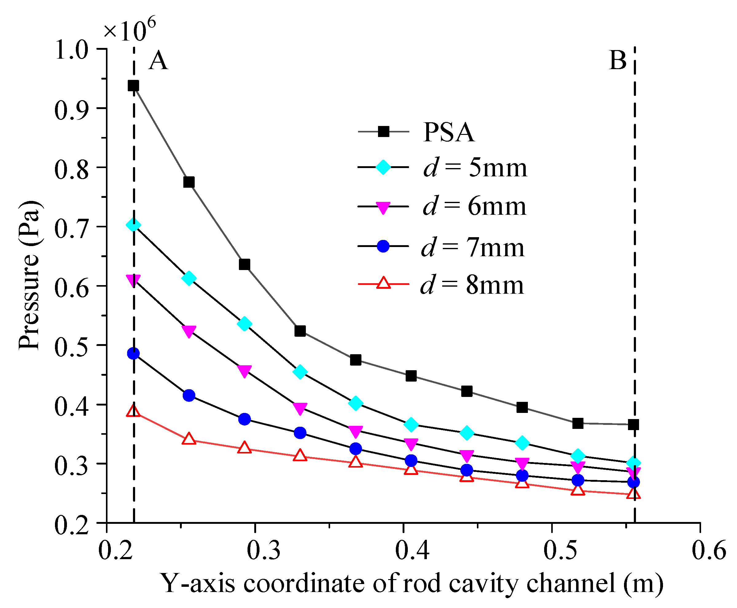
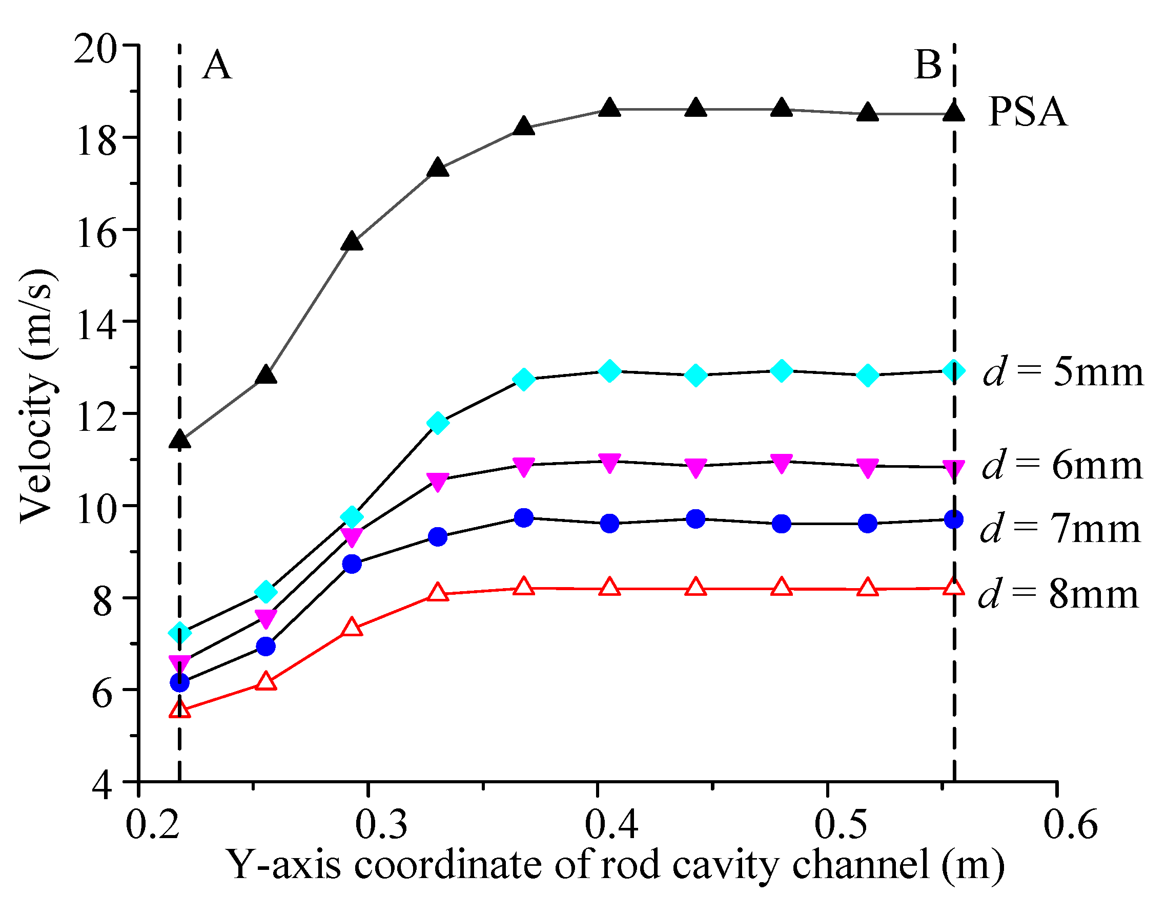
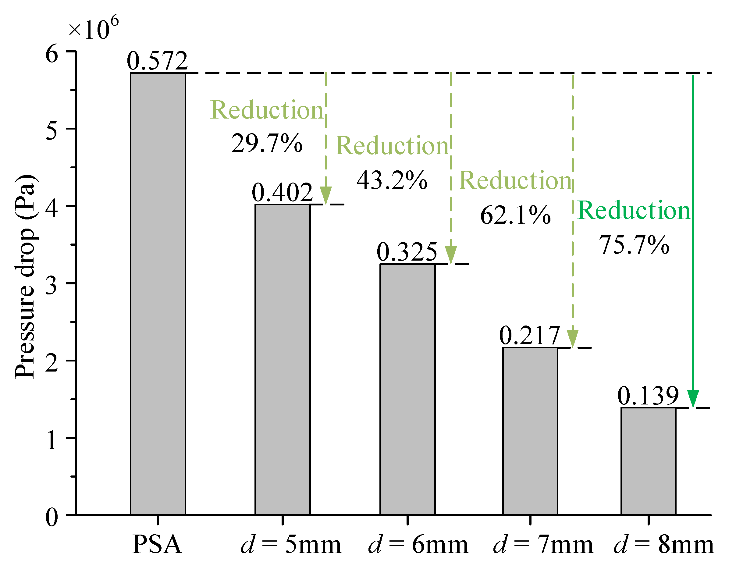
The flow field simulation results indicate that after diameter selection, the pressure loss of the rod cavity channel of the PSA is 0.572 MPa, and the maximum flow speed is 18.63 m/s. Meanwhile, the pressure loss of the rod cavity channel of the APCSA is 0.139 MPa, and the maximum flow speed is 8.19 m/s. Thus, the pressure loss is reduced by 75.7%, and the maximum flow speed is reduced by 56.0%. The effect of the structural redesign is obvious.

(3)

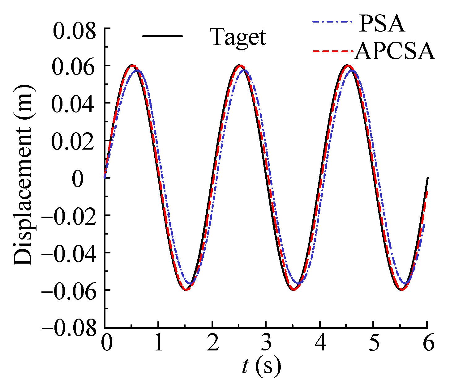
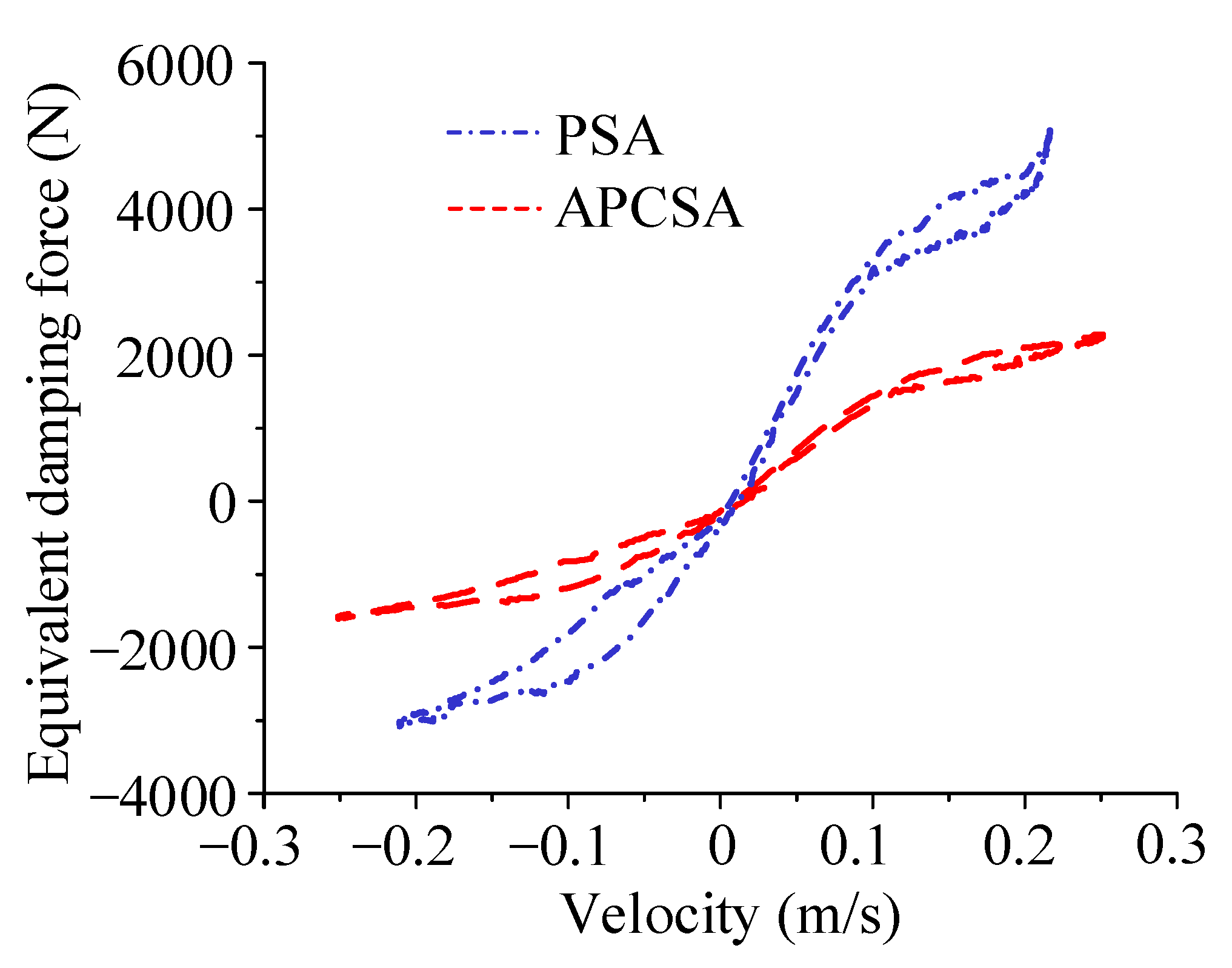
In the step and sinusoidal response experiments, the response velocity and displacement following performance of the APCSA are significantly improved compared with the PSA. The maximum restoring damping force/compression damping force of the APCSA is 2428.98 N/−1470.29 N, which is 53.5%/50.4% lower than that of the PSA. The dynamic response ability of the actuator is improved. The APCSA will assist the active suspension system of the whole vehicle to realize various advanced control algorithms.

References

1. Zhou, C.; Liu, X.H.; Xu, F.X. Intervention criterion and control strategy of active front steering system for emergency rescue vehicle. Mech. Syst. Signal Process. 2021, 148, 107160. [Google Scholar] [CrossRef]
2. Xue, J.; Tu, Q.; Pan, M.; Lai, X.; Zhou, C. An improved energy management strategy for 24t heavy-duty hybrid emergency rescue vehicle with dual-motor torque increasing. IEEE Access 2020, 9, 5920–5932. [Google Scholar] [CrossRef]
3. Li, P.; Yan, J.; Tu, Q.; Pan, M.; Xue, J. A novel energy management strategy for series hybrid electric rescue vehicle. Math. Probl. Eng. 2018, 2018, 1–15. [Google Scholar] [CrossRef] [Green Version]
4. Xu, F.; Liu, X.; Chen, W.; Zhou, C. Dynamic switch control of steering modes for four wheel independent steering rescue vehicle. IEEE Access 2019, 7, 135595–135605. [Google Scholar] [CrossRef]
5. Jeong, K.; Choi, S.B.; Choi, H. Sensor fault detection and isolation using a support vector machine for vehicle suspension systems. IEEE T. Veh. Technol. 2020, 69, 3852–3863. [Google Scholar] [CrossRef]
6. Abdi, B.; Mirzaei, M.; Gharamaleki, R.M. A new approach to optimal control of nonlinear vehicle suspension system with input constraint. J. Vib. Control 2018, 24, 3307–3320. [Google Scholar] [CrossRef]
7. Jing, X.J.; Pan, H.H.; Sun, W.C. Robust finite-time tracking control for nonlinear suspension systems via disturbance compensation. Mech. Syst. Signal Process. 2017, 88, 49–61. [Google Scholar]
8. Shah, D.; Santos, M.M.D.; Chaoui, H.; Justo, J.F. Event-triggered non-switching networked sliding mode control for active suspension system with random actuation network delay. IEEE T. Intell. Transp. early access. 2021. [Google Scholar] [CrossRef]
9. Bai, R.; Guo, D. Sliding-mode control of the active suspension system with the dynamics of a hydraulic actuator. Complexity 2018, 2018, 5907208. [Google Scholar] [CrossRef]
10. Liu, Y.J.; Zeng, Q.; Tong, S.; Chen, C.; Liu, L. Actuator failure compensation-based adaptive control of active suspension systems with prescribed performance. IEEE T. Ind. Electron. 2020, 67, 7044–7053. [Google Scholar] [CrossRef]
11. Attia, T.; Vamvoudakis, K.G.; Kochersberger, K.; Bird, J.; Furukawa, T. Simultaneous dynamic system estimation and optimal control of vehicle active suspension. Vehicle Syst. Dyn. 2019, 57, 1467–1493. [Google Scholar] [CrossRef]
12. Ramalingam, M.; Thirumurugan, M.A.; Kumar, T.A.; Jebaseelan, D.D.; Jebaraj, C. Response characteristics of car seat suspension using intelligent control policies under small and large bump excitations. Int. J. Dyn. Control 2020, 8, 545–557. [Google Scholar] [CrossRef]
13. Enders, E.; Burkhard, G.; Munzinger, N. Analysis of the influence of suspension actuator limitations on ride comfort in passenger cars using model predictive control. Actuators 2020, 9, 77. [Google Scholar] [CrossRef]
14. Han, S.Y.; Zhang, C.H.; Tang, G.Y. Approximation optimal vibration for networked nonlinear vehicle active suspension with actuator time delay. Asian J. Control 2017, 19, 983–995. [Google Scholar] [CrossRef]
15. Li, H.; Gao, H.; Liu, H.; Liu, M. Fault-tolerant h control for active suspension vehicle systems with actuator faults. Part I J. Syst. Control. Eng. 2011, 226, 348–363. [Google Scholar] [CrossRef]
16. Tang, X.; Duan, X.; Gao, H.; Li, X.; Shi, X. CFD investigations of transient cavitation flows in pipeline based on weakly-compressible model. Water 2020, 12, 448. [Google Scholar] [CrossRef] [Green Version]
17. Liu, C.; Li, X.; Li, A.; Cui, Z.; Li, Y. Cavitation onset caused by a dynamic pressure wave in liquid pipelines. Ultrason. Sonochem. 2020, 68, 105225. [Google Scholar] [CrossRef]
18. Abdulkarim, A.H.; Ates, A.; Altinisik, K.; Canli, E. Internal flow analysis of a porous burner via CFD. Int. J. Numer. Method Heat 2019, 29, 2666–2683. [Google Scholar] [CrossRef]
19. Hsu, C.H.; Chen, J.L.; Yuan, S.C.; Kung, K.Y. CFD simulations on the rotor dynamics of a horizontal axis wind turbine activated from stationary. Appl. Mech. 2021, 2, 147–158. [Google Scholar] [CrossRef]
20. Rezaeiha, A.; Montazeri, H.; Blocken, B. CFD analysis of dynamic stall on vertical axis wind turbines using Scale-Adaptive Simulation (SAS): Comparison against URANS and hybrid RANS/LES. Energ. Convers. Manag. 2019, 196, 1282–1298. [Google Scholar] [CrossRef]
21. Yang, X.; Zhou, H.; Wu, H. CFD modelling of biomass ash deposition under multiple operation conditions using a 2D mass-conserving dynamic mesh approach. Fuel 2022, 316, 123250. [Google Scholar] [CrossRef]
22. Mlakar, D.; Winter, M.; Stadlbauer, P.; Seidel, H. Subdivision-specialized linear algebra kernels for static and dynamic mesh connectivity on the GPU. Comput. Graph. Forum 2020, 39, 335–349. [Google Scholar] [CrossRef]
23. Zhu, Q.; Zhang, Y.; Zhu, D. Study on dynamic characteristics of the bladder fluid pulsation attenuator based on dynamic mesh technology. J. Mech. Sci. Technol. 2019, 33, 1159–1168. [Google Scholar] [CrossRef]
24. Salinas, P.; Regnier, G.; Jacquemyn, C.; Pain, C.C.; Jackson, M.D. Dynamic mesh optimisation for geothermal reservoir modelling. Geothermics 2021, 94, 102089. [Google Scholar] [CrossRef]
25. Zheng, Z.; Yang, W.; Yu, P.; Cai, Y.; Zhou, H.; Boon, S.K. Simulating growth of ash deposit in boiler heat exchanger tube based on CFD dynamic mesh technique. Fuel 2020, 259, 1–16. [Google Scholar] [CrossRef]
26. Abdalla, M.O.; Nagarajan, T. A computational study of the actuation speed of the hydraulic cylinder under different ports’ sizes and configurations. J. Eng. Sci. Technol. 2015, 10, 160–173. [Google Scholar]
27. Behrens, B.A.; Hübner, S.; Krimm, R.; Wager, C.; Vucetic, M.; Cahyono, T. Development of a hydraulic actuator to superimpose oscillation in metal-forming presses. Key Eng. Mater. 2011, 473, 217–222. [Google Scholar] [CrossRef]
28. Lai, Q.; Liang, L.; Li, J.; Wu, S.; Liu, J. Modeling and analysis on cushion characteristics of fast and high-flow-rate hydraulic cylinder. Math. Probl. Eng. 2016, 2016, 1–17. [Google Scholar] [CrossRef] [Green Version]
29. Li, S.B.; Liu, Y.L. Numerical simulation on flow field of the rotary cylinder’s spiral flow. Appl. Mech. Mater. 2011, 63, 365–368. [Google Scholar] [CrossRef]
Figure 1. Schematic diagram of mode switching. 1. Body connecting plate. 2. Actuator. 3. Tyre. 4. Servo valve. 5. Mode switching valve block. 6. Accumulator of rodless cavity. 7. Accumulator of rod cavity.
Mathematics 10 04303 g001
Figure 2. Actuator structure model. 1. Rod cavity. 2. Rodless cavity. 3. Rodless cavity channel. 4. Rod cavity channel.
Mathematics 10 04303 g002
Figure 3. Mesh sensitivity check.
Mathematics 10 04303 g003
Figure 4. Fluid domain mesh model.
Mathematics 10 04303 g004
Figure 5. Pressure contour: (a) t = 0 s; (b) t = 0.2 s; (c) t = 0.4 s; (d) t = 0.67 s.
Mathematics 10 04303 g005aMathematics 10 04303 g005b
Figure 6. Pressure curve of the rod cavity channel.
Mathematics 10 04303 g006
Figure 7. Velocity contour: (a) t = 0 s; (b) t = 0.2 s; (c) t = 0.4 s; (d) t = 0.67 s.
Mathematics 10 04303 g007aMathematics 10 04303 g007b
Figure 8. Velocity curve of rod cavity channel.
Mathematics 10 04303 g008
Figure 9. Structural model and fluid domain mesh model: (a) structure model; (b) mesh model. 1. Rod cavity. 2. Rodless cavity. 3. Rodless cavity channel. 4-1. Rod cavity channel. 4-2. Rod cavity channel (d = 5, 6, 7, 8 mm).
Mathematics 10 04303 g009aMathematics 10 04303 g009b
Figure 10. Pressure curve at different diameters.
Mathematics 10 04303 g010
Figure 11. Velocity curve at different diameters.
Mathematics 10 04303 g011
Figure 12. Comparison of pressure drop at different diameters.
Mathematics 10 04303 g012
Figure 13. Comparison of flow speed at different diameters.
Mathematics 10 04303 g013
Figure 14. Pressure contour: (a) t = 0 s; (b) t = 0.2 s; (c) t = 0.4 s; (d) t = 0.67 s.
Mathematics 10 04303 g014aMathematics 10 04303 g014b
Figure 15. Velocity contour: (a) t = 0 s; (b) t = 0.2 s; (c) t = 0.4 s; (d) t = 0.67 s.
Mathematics 10 04303 g015aMathematics 10 04303 g015b
Figure 16. Suspension actuator test bench: (a) actuating bench; (b) pump station.
Mathematics 10 04303 g016
Figure 17. Actuator structure comparison diagram: (a) PSA; (b) APCSA.
Mathematics 10 04303 g017
Figure 18. Displacement step response: (a) response comparison curve; (b) rise time comparison chart.
Mathematics 10 04303 g018
Figure 19. Displacement square wave response: (a) response comparison curve; (b) rise time com parison chart.
Mathematics 10 04303 g019
Figure 20. The 0.5 Hz sinusoidal response.
Mathematics 10 04303 g020
Figure 21. The 1 Hz sinusoidal response.
Mathematics 10 04303 g021
Figure 22. Different output force curves: F1 is the theoretical output force of the PSA; N1 is the actual output force; F2 is the theoretical output force of the APCSA; N2 is the actual output force.
Mathematics 10 04303 g022
Figure 23. Equivalent damping force.
Mathematics 10 04303 g023
Figure 24. Equivalent damping force–displacement curve.
Mathematics 10 04303 g024
Figure 25. Equivalent damping force–velocity curve.
Mathematics 10 04303 g025