Article

Improved Large Covariance Matrix Estimation Based on Efficient Convex Combination and Its Application in Portfolio Optimization

1
School of Mathematics, Physics and Statistics, Shanghai University of Engineering Science, Shanghai 201620, China
2
Department of Mathematics and Statistics, Loyola University Maryland, Baltimore, MD 21210, USA
*
Author to whom correspondence should be addressed.
Mathematics 2022, 10(22), 4282; https://doi.org/10.3390/math10224282
Submission received: 24 October 2022 / Revised: 12 November 2022 / Accepted: 13 November 2022 / Published: 16 November 2022
(This article belongs to the Special Issue Applied Computing and Artificial Intelligence)

Abstract

:
The estimation of the covariance matrix is an important topic in the field of multivariate statistical analysis. In this paper, we propose a new estimator, which is a convex combination of the linear shrinkage estimation and the rotation-invariant estimator under the Frobenius norm. We first obtain the optimal parameters by using grid search and cross-validation, and then, we use these optimal parameters to demonstrate the effectiveness and robustness of the proposed estimation in the numerical simulations. Finally, in empirical research, we apply the covariance matrix estimation to the portfolio optimization. Compared to the existing estimators, we show that the proposed estimator has better performance and lower out-of-sample risk in portfolio optimization.

1. Introduction

With the development of information technology, the covariance matrix estimation plays a crucial role in multivariate statistics analysis, and it is used widely in many fields, such as finance, wireless communications, biology, chemometrics, social networks, health sciences, etc. [1,2,3,4,5]. In particular, due to the high noise of the sample covariance matrix, the properties of financial data are not characterized by multivariate normality and stationarity [6]. As an essential input to many financial models, it is vital to remove the sample noise to improve the estimation accuracy of the covariance matrix in asset allocation and risk management [4,7,8]. It is known that the sample covariance matrix is no longer a good estimator of the population covariance matrix when the dimension of the matrix is close to or larger than the sample size. In fact, the sample covariance matrix becomes a singular matrix in high-dimensional data. The so-called “high dimensions” mainly include large orders of 30 in magnitude and high data dimensions [1,2,3]. So far, some popular ways used to obtain a good estimator are the shrinkage estimation methods without prior information, sparse estimation methods with prior information, the factor model [9,10], the rank model [11], etc.
The shrinkage method, proposed by Stein [12], is one without prior information for estimating the covariance matrix. The essential idea of this method is to pull extreme eigenvalues of the sample covariance matrix toward the mean of the eigenvalues by shrinking the eigenvalues when the dimension of the matrix is close to the sample size. Ledoit and Wolf showed that the shrinkage estimation methods have an improvement over the sample covariance matrix. Specifically, they proposed the shrinkage estimation methods provide good solutions to deal with the overfitting of the sample covariance matrix [8,13,14].
Since the linear shrinkage method is the first-order approximation to a nonlinear problem, as the dimension of the matrix becomes high, it is no longer suitable for the improvement of the sample covariance matrix. Thus, they proposed the nonlinear shrinkage method [15], which has better performance for high-dimensional asymptotics. Recently, Ledoit and Wolf proposed optimal nonlinear shrinkage estimators [16], which are decision-theoretically optimal within a class of nonlinear shrinkage estimators. For more details on the shrinkage methods, refer to [2,3,17,18].
The sparse estimation with prior information is another one for estimating the covariance matrix, which estimates the sparse matrix directly and its inverse indirectly. In the case of direct estimation, Bickel and Levina [19] showed that the estimation can be obtained by the threshold methods under the hypothesis of the sparseness of the true covariance matrix. In the case of no assumption of the sparse pattern, Rothman et al. [20] proposed a new class of generalized threshold estimators to obtain the sparse estimation by inducing sparsity and imposing the norm penalty. Theoretically, these methods are shown to be superior, and the generalized thresholding estimators are consistent with a large class of approximate sparse covariance matrices. In fact, the resulting estimators are not always positive-definite. In order to guarantee the positive definiteness of the covariance matrix estimation, Rothman et al. [21] built a convex optimization model based on the quadratic loss function under the Frobenius norm (F-norm) and studied the estimation of the high-dimensional covariance matrix. Subsequently, some convex optimization models with penalty functions such as the L 1 function were proposed [22,23], and some nonconvex penalty functions were used to achieve both sparsity and positive definiteness [24,25]. However, since the changes of the variance and covariance over time are not considered, they are affected by dimensional disasters and large noise problems. For more details about optimization algorithms and inverse matrix estimation methods, refer to the literature [7,26,27,28,29,30,31] and the references therein.
In addition, Bun et al. [32] introduced the rotation-invariant estimation in which they assumed that the estimator of the population correlation matrix shares the same eigenvectors as the sample covariance matrix itself. The experiments’ results demonstrated that the rotation-invariant estimator is more suitable for dealing with large dimension datasets than the eigenvalue clipping methods and can be significantly improved over the sample covariance matrix as the data size grows, but it did not perform well on a small sample data. In a recent paper [33], Deshmukh et al. combined the shrinkage transformation with the eigenvalue clipping to obtain the estimator of the covariance matrix for the convex combination of the optimal parameters. This estimator can achieve less out-of-sample risk in portfolio optimization for small datasets.
The research in this paper was mainly motivated by [32,33], and the novelties of this study are as follows:
  • A new large covariance matrix estimator is proposed by constructing a convex combination of the linear shrinkage estimation and the rotation-invariant estimator under the Frobenius norm.
  • Our new covariance matrix estimator improves the impact of the sample noise on the covariance matrix by adjusting the parameters of the convex combination in financial data.
  • The proposed estimator has better performance and lower out- of-sample risk in portfolio optimization.
The rest of this paper is organized as follows: Section 2 describes the related work of covariance matrix estimation. Section 3 introduces our new proposed estimator and its application. Section 4 implements the numerical simulation and empirical research. Section 5 gives the conclusions.

2. Preliminaries

2.1. The Rotation-Invariant Estimator

First, we briefly introduce the basic idea of the rotation-invariant estimator. For more details, we refer to [32].
Let r = ( r 1 , r 2 , . . . , r N ) denote a T × N matrix of T independent and identically distributed (iid) observations on a system of N random variables with mean vector μ . N and T denote the number of variable and the size of the variable, respectively. In this case, the sample covariance matrix is given by
Σ S C M = ( σ i j ) = 1 N 1 i = 1 N ( r i μ ) ( r i μ ) ,
Let N and T be asymptotic in the high-dimensional regime, i.e.,
N T .
In addition, the concentration ratio is given by
c = N T .
The construction steps of the rotation-invariant estimator are as follows:
  • Step 1: Calculate the Stieltjes transform of the empirical spectral measure of S 1 from
    s ( z ) = 1 T T r ( S 1 z ) 1
    where z denotes the spectral parameter and
    S 1 = 1 N 1 i = 1 N ( r i μ ) ( r i μ ) ,
    The function (4) contains all the information about the eigenvalues of the matrix S 1 , which has the same nonzero eigenvalues as Σ S C M .
  • Step 2: Update (4) based on the nonzero eigenvalues of Y Y and Y Y , i.e.,
    s ( z ) = 1 T T r ( S 1 z ) 1 ,
    where y i = r i μ , Y = ( y 1 , y 2 , . . . , y N ) , and λ i denotes the ith eigenvalue of the sample covariance matrix Σ S C M .
  • Step 3: Calculate the function δ ^ i of the ith eigenvalue of S from
    δ i ^ = 1 λ i | s ( λ i + i η ) | 2 .
    where s ( · ) is the empirical Stieltjes transform from (6) and parameter η = T 1 2 .
  • Step 4: Output the resulting covariance matrix estimator Σ R I E from
    Σ R I E = U N D ^ N U N ,
    where
    D ^ N = D i a g ( λ ^ 1 , λ ^ 2 , . . . , λ ^ N ) ,
    U N is an orthogonal matrix, whose columns [ u 1 , u 2 , . . . , u N ] are the corresponding eigenvectors, with the eigenvalue of the rotation-invariant estimator defined by
    λ i ^ = i = 1 N λ i i = 1 N δ i ^ δ i ^ .
One can easily verify that
i = 1 N λ i ^ = i = 1 N λ i .
This implies that the estimator Σ R I E has the same trace as the sample covariance matrix. More literature reviews on rotation-invariant estimators are presented in the Table 1.

2.2. Improved Covariance Estimator Based on Eigenvalue Clipping

Deshmukh et al. [33] introduced an improved estimation based on eigenvalue clipping, which takes the optimal parameters in the convex combination of the sample covariance matrix Σ S C M , the shrinkage target Σ F
Σ F = ( f i j ) ,
with
f i j = 2 σ i i σ j j N ( N 1 ) i = 1 N 1 j = i + 1 T σ i j σ i i σ j j , i j , σ i i , i = j ,
and the matrix Σ M P obtained by applying eigenvalue clipping.
Let y i = r i r ¯ i be independent, identically distributed, random variables with finite variance σ . The Marchenko–Pastur density ρ Σ S C M ( λ ) of the eigenvalues of Σ S C M is defined by
ρ Σ S C M ( λ ) = 1 N d n ( λ ) d λ .
where n ( λ ) is the number of eigenvalues of the sample covariance matrix Σ S C M less than λ .
In the condition of the limit N , T , and 1 c 1 , the density follows from (14):
ρ Σ S C M ( λ ) = 1 2 π c σ 2 ( λ m a x λ ) ( λ λ m i n ) λ ,
where
λ m a x = σ 2 ( 1 + c + 2 c ) , λ m i n = σ 2 ( 1 + c 2 c ) .
[ λ m i n , λ m a x ] represents the MP law bounds. In this case, the covariance matrix can be cleaned by scaling the eigenvectors of Σ S C M with these new eigenvalues. Σ M P is obtained by this method.
Let Σ be the population covariance matrix; the optimal parameters in convex combination can be found from the following optimization problem [33].
min θ , ϕ | | Σ Σ e s t | | F
s . t . Σ e s t = ϕ ( θ Σ F + ( 1 θ ) Σ M P ) + ( 1 ϕ ) Σ S C M , 0 θ 1 , 0 ϕ 1 .
where θ and ϕ are the parameters of the convex combination.
Usually, the eigenvectors of the sample covariance matrix deviate from those of the population covariance matrix under large-dimensional asymptotics. Correcting the deviation of the eigenvalues of the sample covariance matrix can improve the performance of the large covariance matrix. Although the estimation can adapt to changing the sampling noise conditions by performing parameter optimization, the performance of the estimation outperforms other estimations only for small-dimensional problems.

3. Proposed Estimator and Application in Portfolio Optimization

3.1. Proposed Estimator

For further improve the performance of the large covariance matrix, we replaced the eigenvalues falling inside Marchenko–Pastur (MP) law bounds with the rotation-invariant estimator Σ R I E and applied the linear shrinkage estimation to shrink the eigenvalues falling outside the MP law bounds in this paper. Our new estimation is presented below.
min θ , ϕ | | Σ Σ e s t | | F
s . t . Σ e s t = ϕ ( θ Σ F + ( 1 θ ) Σ R I E ) + ( 1 ϕ ) Σ S C M , 0 θ 1 , 0 ϕ 1 ,
Thus, the estimation of the covariance matrix is given by
Σ * = ϕ * ( θ * Σ F + ( 1 θ * ) Σ R I E ) + ( 1 ϕ * ) Σ S C M .
where θ * and ϕ * are the optimal parameters of the optimization problem given by (19) and (20).
It is well known that the financial data are heavy-tailed and non-normal [7,33]. However, the existing covariance matrix estimation methods generally requires the assumption of normality [32,38]. For overcoming this drawback, we propose a new estimator, which is a convex combination of the linear shrinkage estimation and the rotation-invariant estimator under the Frobenius norm. One advantage of the new estimation is that we can remove the noise caused by the bulk eigenvalues and the extreme eigenvalues in the financial data. Furthermore, we set five-fold cross-validation k = 5 to implement the simulation and empirical research for improving the accurate estimation of the covariance matrix.
The detailed steps of our new estimation are as follows.
  • Step 0: Input the sample data r = ( r 1 , r 2 , . . . , r N ) , and set k = 1 .
  • Step 1: Calculate Σ S C M , Σ F , and Σ R I E from (5), (12), and (8), respectively.
  • Step 2: Calculate Σ e s t from (20), and denote Σ e s t ( θ i , ϕ j ) for θ i , ϕ j , i = 1 , 2 , . . . , M , j = 1 , . . . , P , where M and P are the numbers of θ and ϕ taken between 0 and 1, respectively.
  • Step 3: Calculate the error:
    Δ k ( θ i , ϕ j ) = | | Σ e s t ( θ i , ϕ j ) Σ | | F ,
    for θ i , ϕ j , i = 1 , 2 , . . . , M , j = 1 , . . . , P , and let k = k + 1 .
  • Step 4: Repeat Steps 1–3 in the cross-validation until the folds k = 5 .
  • Step 5: Find the optimal parameters θ * and ϕ * in the convex combination from the corresponding smallest error sum Δ s u m given by
    Δ s u m = k = 1 5 i = 1 M j = 1 P Δ k ( θ i , ϕ j ) .
  • Step 6: Output the proposed estimation Σ * from (21).

3.2. Minimum Variance Portfolio Optimization

According to Markowitz’s theory [39], we included an additional return constraint in the portfolio because even a risk-averse investor would expect a minimal positive return. The classic portfolio optimization model that satisfies the minimum expected return is defined by
min x x Σ x
s . t . 1 x = 1 , r x r m i n , x 0 ,
where x, r, and r m i n represent the weight of portfolio optimization, daily return, and the minimum daily expected return, respectively. It is well known that the portfolio selection is widely used in the financial field, which is a convex quadratic programming problem [39].
In the portfolio optimization, the weight of each asset is closely related to the covariance matrix. An accurate covariance matrix can achieve a more reasonable weight distribution and better portfolio effect. Due to the heavy-tailed nature of financial data and the availability of limited samples [8], many studies started concentrating on the global minimum variance (GMV) portfolio. To improve the performance of the sample covariance matrix in the portfolio optimization, DeMiguel [40] added the additional constraint and regularizing asset weight vector into the minimum variance portfolio and showed that the estimator always leads the constructed portfolio to achieve a smaller variance and a higher Sharpe ratio than other portfolios. Furthermore, Ledoit and Wolf [18] applied the estimation to the portfolio optimization to overcome the dimension and noise problems of a high-dimensional covariance matrix, and the results were better than the linear shrinkage estimation [13]. Moreover, due to the influence of financial market information on covariance matrix estimation, the time-varying covariance matrix or the correlation matrix also have practical significance in portfolio optimization. For more details, refer to [41] and the references therein.
In this paper, we divided the sample data into in-sample data and out-of-sample data, which were used for the estimation and prediction of the covariance matrix, respectively. To measure the out-of-sample performance of the estimation of the covariance matrix in portfolio optimization, we used the out-of-sample risk, the average return, and the Sharpe ratio as the criteria of the measurement. The average return was annualized by multiplying it by 252 (252 trading days per year), and the standard deviation was annualized by multiplying it by 252 . The out-of-sample performance of the portfolio model was evaluated through the following procedure.
  • Step 0: Input the returns of the current in-sample r i n and out-of-sample data r o u t , the expected return r m i n , and the estimation of the covariance matrix Σ * .
  • Step 1: Set r : = r i n , and solve the optimal weight vector x * from Model (22) by the quadratic optimizer called quadprog in Matlab.
  • Step 2: Calculate the out-of-sample Σ ^ * from (21), and obtain the out-of-sample standard deviation:
    σ o u t = v a r ( ( x * ) r o u t ) ,
    the average return:
    r a v e = E ( ( x * ) r o u t ) ,
    and the Sharpe Ratio:
    S R = r a v e r f σ o u t
    where x * and r f represent the optimal weight vector and the risk-free interest, respectively.

4. Numerical Simulation and Empirical Research

4.1. Numerical Simulation

In the simulation, we used the simulation data of Engle et al. [41], and the mean return ranged between −0.0031 and 0.0036. We divided the dataset into in-sample data and out-of-sample data, and both the sample sizes were T = 500 . In pursuit of accuracy, we implemented the five-fold cross-validation, and the parameter selection criterion was the F-norm of the estimator and the population covariance matrix. We set three dimensions for the return series, which were N = 100 , 200 , and 400, respectively. The maximum concentration ratio is
c = N T = 400 500 = 0.80 .
To measure the performance of the estimators, we compared the error between each estimator and the population covariance matrix. The six estimators are shown in Table 2.
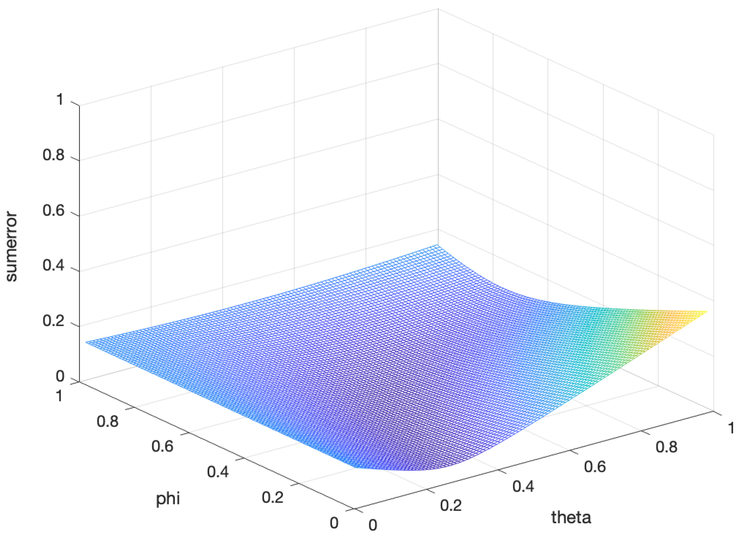
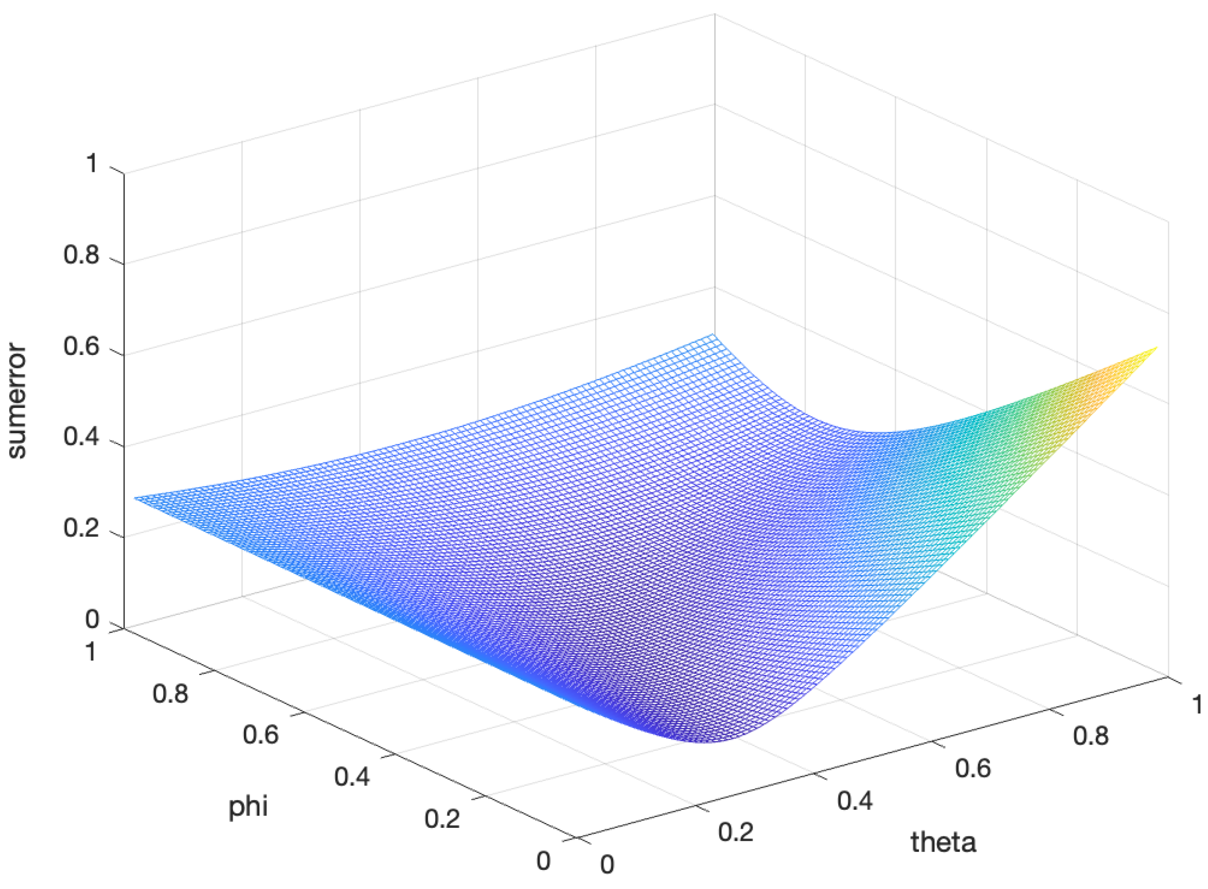
In the five-fold cross-validation, we obtained the error between the proposed estimation and the population covariance matrix for the different parameters θ and ϕ under three asset dimensions. In Figure 1, Figure 2 and Figure 3, the horizontal and longitudinal axis represent the different values of θ and ϕ , respectively, and the vertical axis represents the sum of the error. It is obvious that there are two optimal parameters to minimizing the error between the proposed estimator and the population covariance matrix for all θ and ϕ . The results are shown in Table 3. To some degree, this ensures the effectiveness of the proposed estimation.
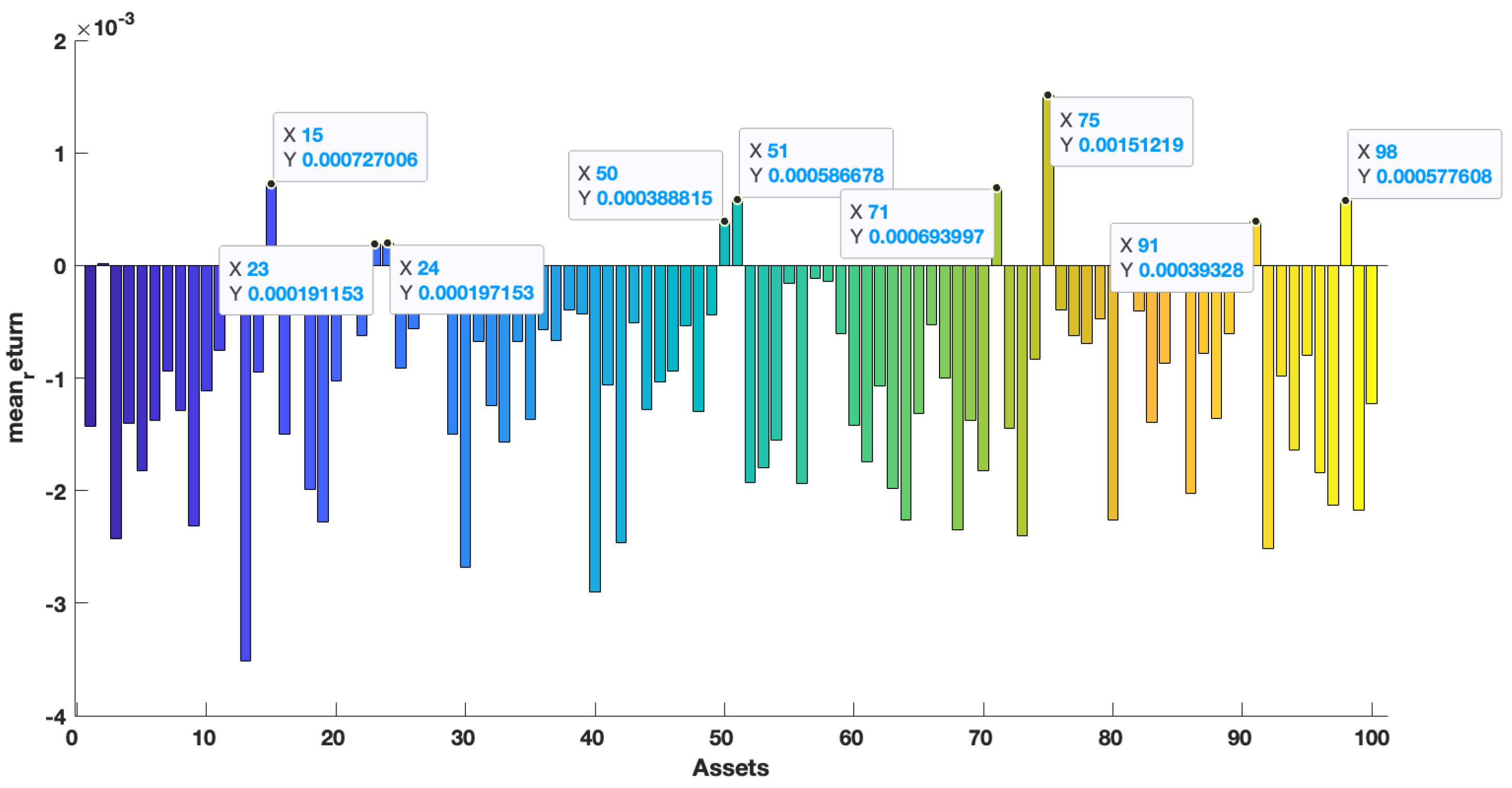
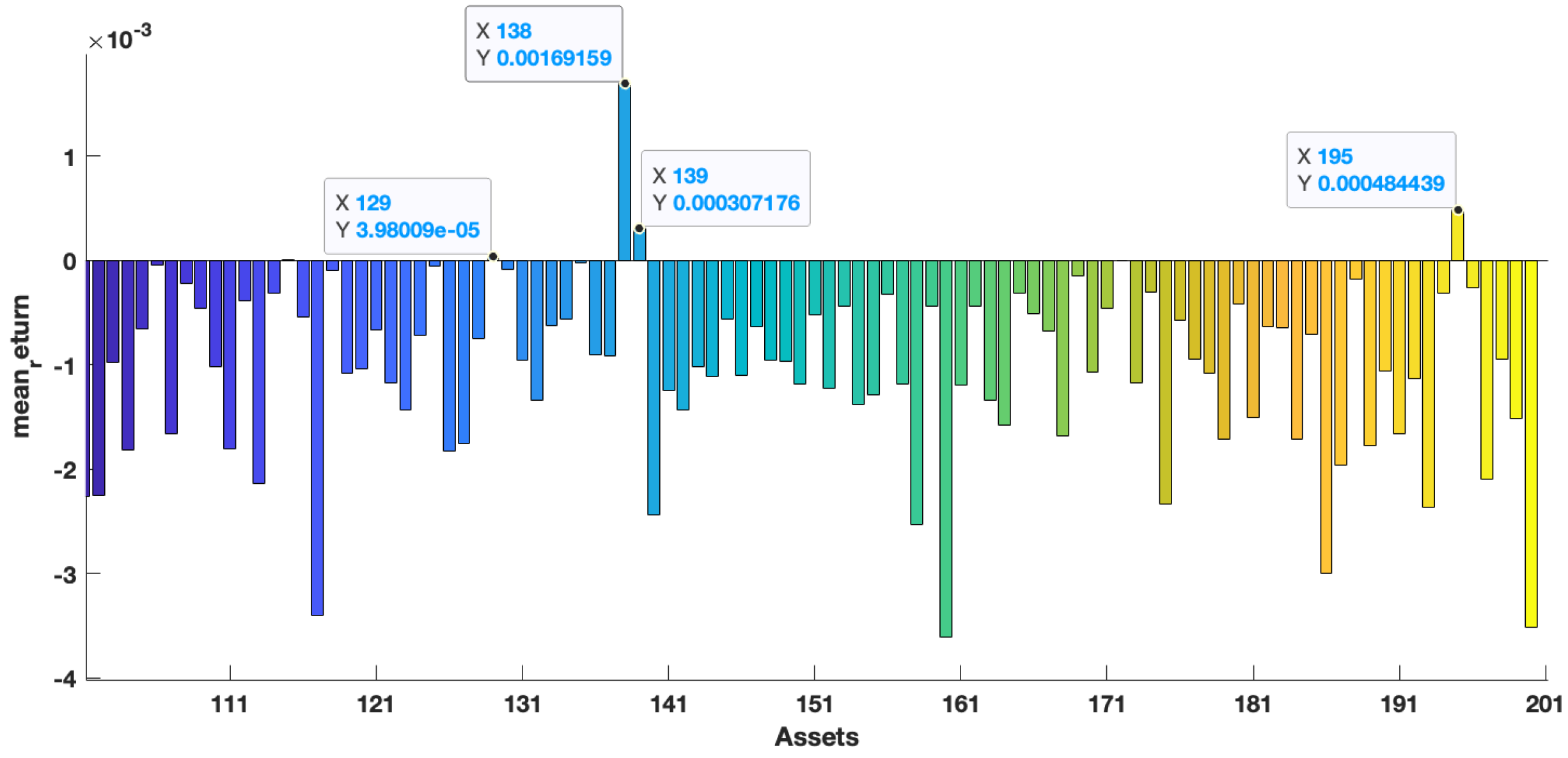
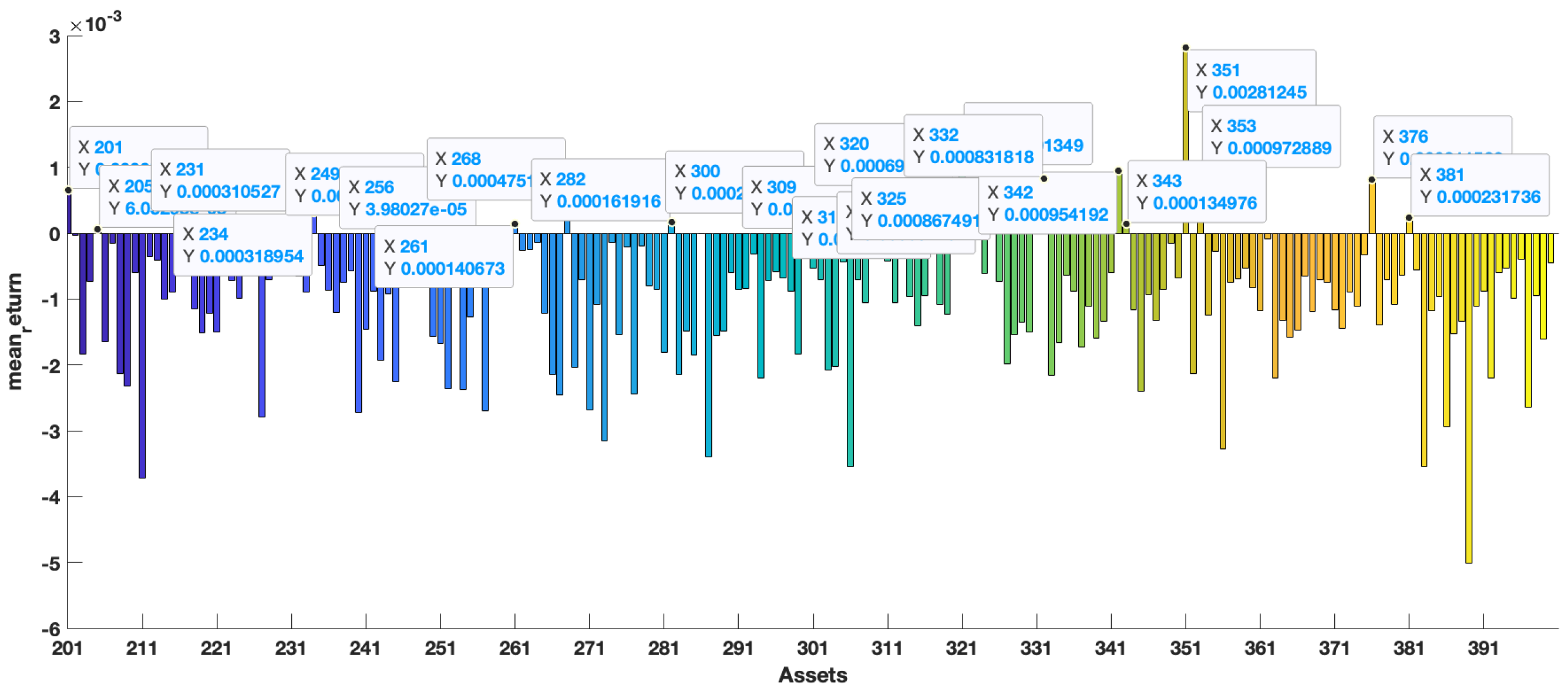
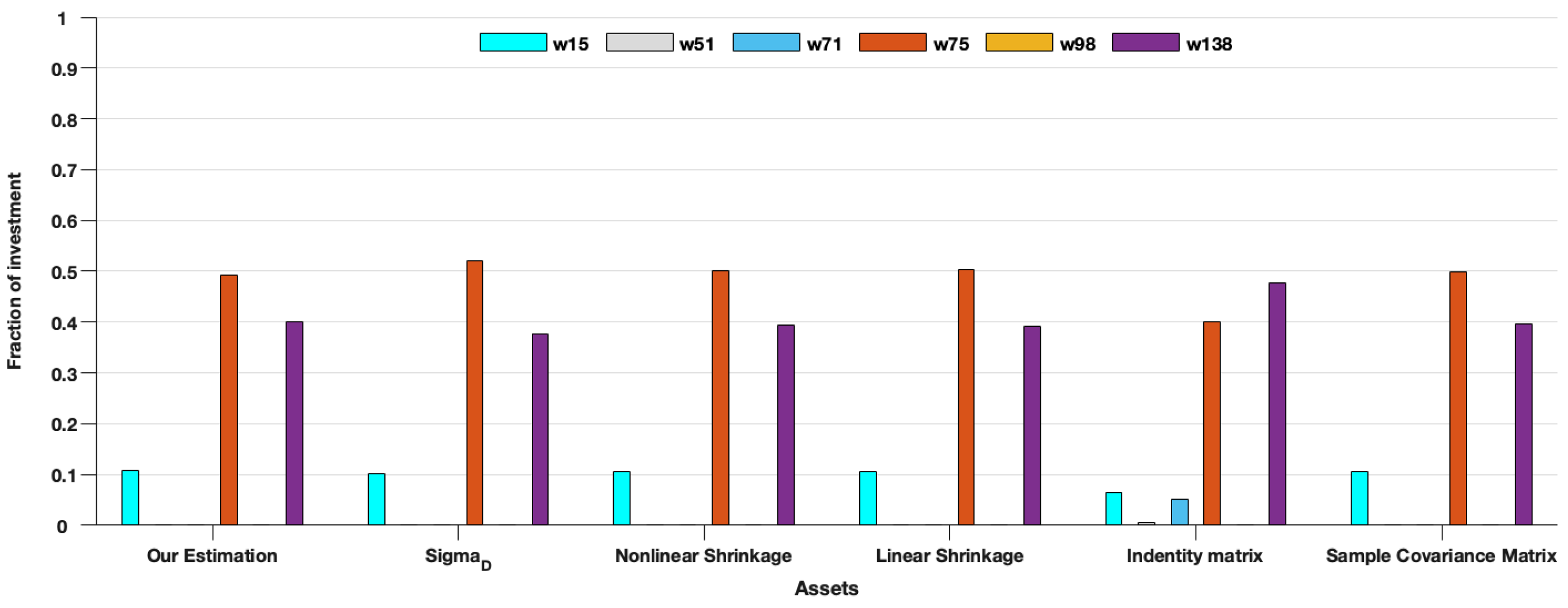
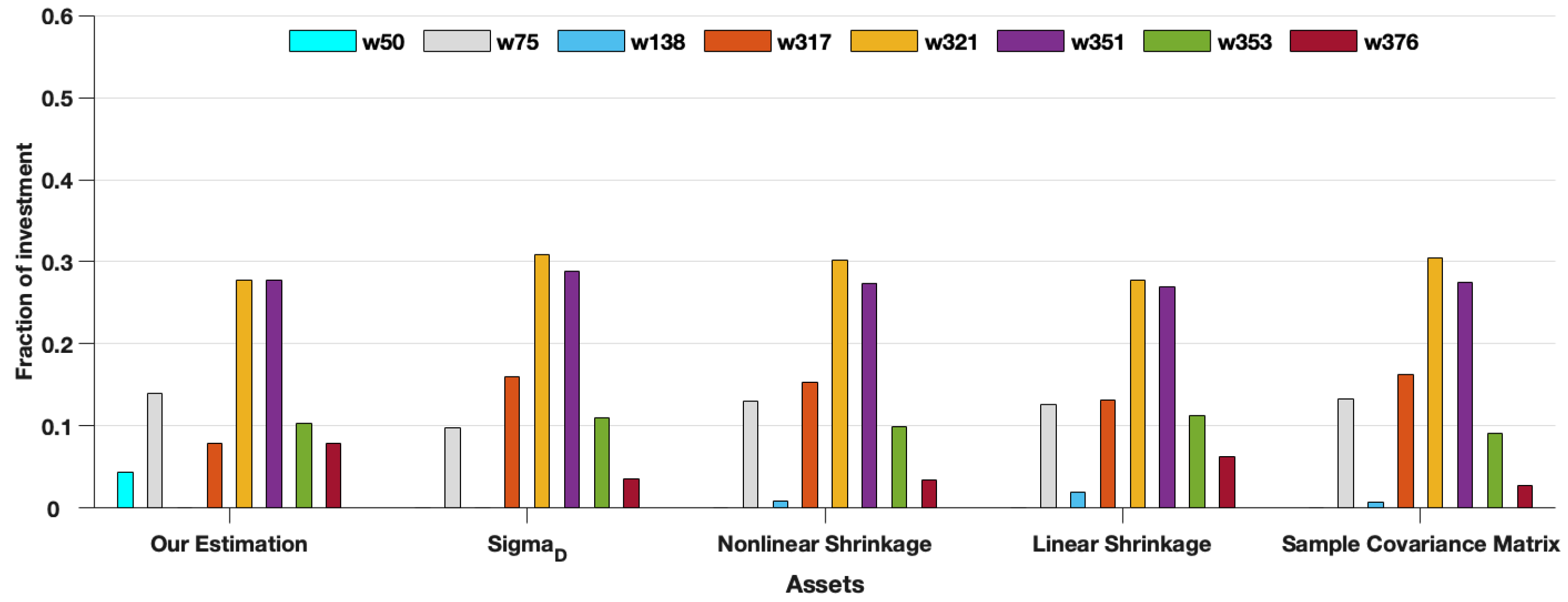
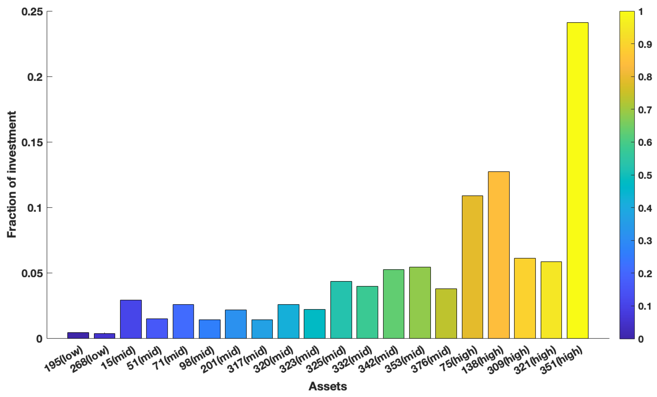
Table 4 shows that the F-norm error of our new estimation is the smallest in the ones of the six estimations. Under this premise, we calculated the portfolio variance in the minimum variance portfolio that satisfies the minimum 0.0015 expected return. The results are shown in Table 5. Figure 4, Figure 5 and Figure 6 show the mean return of out-of-sample data ranging from the 1st asset to the 400th asset. We mark individual points on the graph. The horizontal and longitudinal axis represent the order of assets in the total assets and the mean return of this asset, respectively. We can see that the mean return of the point that is marked is relatively high. Generally speaking, higher asset returns will also face relatively large investment risks. To understand the following description, we divided the return into three asset risk grades: high ( r m i n 0.001 ), middle ( 0.0005 r m i n 0.001 ), and low ( r m i n < 0.0005 ), respectively. In Table 5, it is obvious that the variance of Σ I d e n t i t y is the largest in all asset dimensions. In the case of N = 200 , the asset weights of the portfolio model corresponding to Σ I d e n t i t y are distributed on the 15th, 51st, 71st, 75th, and 138th assets in Figure 7, respectively, with 87 % high-risk assets and 13 % medium assets. However, in the case of N = 400 , the asset weights of the portfolio model corresponding to Σ I d e n t i t y are distributed on twenty assets, with 60 % high-risk assets, 39.5 % medium assets, and only 0.5 % low-risk assets, and we can see that the high-risk and medium-risk assets account for the vast majority of the 20 assets. Instead, the portfolio model corresponding to our new estimator Σ * distributed the weights on high-risk assets and medium-risk assets as 69 % and 26.12 % , respectively, to achieve the 0.0015 expected return. The remaining 5 % was distributed on low-risk assets to reduce investment risk. The corresponding results are shown in Figure 8 and Figure 9. Overall, the reasonable distribution of asset weights on high-, medium, and low-risk assets can appropriately decrease investment risks. As the number of the assets increased, the performance of our new estimator Σ * became better. At the same time, the proposed estimation in the minimum variance portfolio was more dispersed on the allocation of the assets.

4.2. Empirical Research

The data of this paper came from the component stock of CSI500, HS300, and SSE50 on the tushare financial website. The whole period of the samples was from 24 May 2017 to 1 July 2021. Removing the missing data of the samples from transaction, we finally obtained 426 component stocks of CSI500, 218 component stocks of HS300, and 41 component stocks of SSE50.
In this paper, we set T 1 = 500 and T 2 = 500 as the window of estimation and prediction, respectively. The maximum concentration ratio is
c = N T 1 = 426 500 = 0.852 .
We used the log return as we studied the object and divide all samples into two parts for estimation and prediction. We constructed six portfolio optimization models by using the estimator in Table 2. The procedures of estimation and prediction are as follows.
  • Step 0: Input the sample data; divide the data into in-sample data T 1 = 500 and out-of-sample data T 2 = 500 .
  • Step 1: Calculate Σ F , Σ R I E , and Σ S C M based on the in-sample data.
  • Step 2: Set five-fold cross-validation; calculate the Σ e s t from (20) for parameters between 0 and 1; implement the minimum variance portfolio (22), where r m i n takes a value from the minimum to maximum mean return; solve the corresponding weight vector x by multiple times of iteration over the values of both θ and ϕ in the convex optimization.
  • Step 3: Calculate the standard deviation based on the out-of-sample data, and record the out-of-sample risk σ o u t in each iteration.
  • Step 4: Calculate the optimal parameters θ * , ϕ * when the sum of σ o u t of the five-fold cross-validation achieves the minimum.
  • Step 5: Implement the minimum variance portfolio (22) to obtain the assets’ weights, the average return r a v e , and the out-of-sample risk σ r i s k when satisfying the minimum 0.002 return constraints under the θ * and ϕ * .
  • Step 6: Calculate the Sharpe ratio, where the risk-free interest is set as 1.75 % .
In portfolio optimization, the reduction of volatility at the first decimal place is also considered to be quite significant [13,33]. Table 6 and Table 7 show the performance of the six portfolio optimization model based on the different asset dimensions. For out-of-sample data, we used the standard deviation as the performance metric. Furthermore, we calculated the average return and the Sharpe ratio in the portfolio optimization model (22) and the risk-free interest was set to 1.75%.
Table 6, Table 7 and Table 8 show that the average returns of each estimator are equal. Table 6 shows that the standard deviation of the portfolio optimization model corresponding to Σ I d e n t i t y is only 27.53 % , which is the smallest in each estimator. The standard deviation of the portfolio optimization model corresponding to our new estimator Σ * is 27.97%, and its performance ranks fourth among all estimators.
Table 7 shows the performance of the portfolio optimization model corresponding to each estimator with 218 assets. It can be seen that the performance of the estimator Σ I d e n t i t y becomes weak. In this case, Σ I d e n t i t y is the worst estimator, which is expected as it assumes zero correlations among stocks, and Σ S C M is the second-worst. The Sharpe ratio of the portfolio optimization corresponding to Σ N L is the highest in each estimator followed by the one of Σ D . At the same time, the performance of our new estimator Σ * ranks third among all estimators. Comparing to the case of N = 218 , the performance of our new estimator improved as the asset dimension increased.
Table 8 compares the performance of each model with the number of assets of 426. The result shows that the portfolio optimization model corresponding to our new estimator Σ * obtaining the smallest standard deviation leads to the highest Sharpe ratio. Obviously, compared with other estimators, especially with Σ I d e n t i t y , our new estimator has a significant decrease in the out-of-sample standard deviation. Meanwhile, this also implies that the performance of our new estimator Σ * is superior to the ones of the other five estimators as the asset dimension increases.
The homogeneity of the variance test is a metric to measure whether the variances of the two investment strategies are equal, and we used the improved bootstrap inference [44] to test the significant variance difference between Σ * and other estimations excess returns. Table 9 shows that the test between Σ * and the alternative methods all reject the null hypothesis of equal variances. Moreover, the sample variance of the excess return generated corresponding to our new estimator Σ * is significantly lower than the other portfolio optimization models as the number of assets increases. Therefore, our new estimation Σ * is superior to other estimations.

5. Conclusions

In this paper, we proposed a new estimator for the covariance matrix, which is a convex combination of the linear shrinkage estimation and the rotation-invariant estimator under the F-norm. We first obtained the optimal parameters through considerable numerical operations, and then, we focused on the accuracy of the model and ignored the complexity of the calculation. Moreover, we demonstrated the effectiveness of the model in the simulation. Finally, we applied our estimation to the minimum variance portfolio optimization and showed that the performance of the proposed estimator is superior to the other five existing estimators in the portfolio optimization for high-dimensional data.
In addition, we only considered the sample noise on the covariance matrix in this article, but in the financial field, the covariance matrix estimation will vary with time due to the influence of market information, and the covariance matrix estimation will be affected by the market information. Therefore, the performance of our new estimation in the dynamic conditional correlation model [41] can be investigated as part of future work for a large-dimensional covariance matrix.

Author Contributions

Conceptualization, Y.Z.; Fund acquisition, G.W. and Z.Y.; methodology, Y.Z. and J.T.; supervision, G.W. and Z.Y.; writing—original draft preparation, Y.Z.; writing—review and editing, Y.Z., J.T. and G.W. All authors have read and agreed to the published version of the manuscript.

Funding

This research was funded by the National Natural Science Foundation of China (Nos. 11971302 and 12171307).

Informed Consent Statement

Not applicable.

Data Availability Statement

The data of this paper came from the component stock of CSI500, HS300, and SSE50 on the tushare financial website accessed on 1 July 2021: https://www.tushare.pro.

Conflicts of Interest

The authors declare no conflict of interest.

References

  1. Hu, J.; Bai, Z.D. A review of 20 years of naive tests of significance for high-dimensional mean vectors and covariance matrices. Sci. China Math. 2016, 59, 2281–2300. [Google Scholar] [CrossRef] [Green Version]
  2. Tong, T.; Wang, C.; Wang, T. Estimation of variances and covariances for high-dimensional data: A selective review. Wiley Interdiscip. Rev. Comput. Stat. 2014, 6, 255–264. [Google Scholar] [CrossRef] [Green Version]
  3. Engel, J.; Buydens, L.; Blanchet, L. An overview of large-dimensional covariance and precision matrix estimators with applications in chemometrics. J. Chemom. 2017, 31, e2880. [Google Scholar] [CrossRef]
  4. Sun, R.; Ma, T.; Liu, S.; Sathye, M. Improved covariance matrix estimation for portfolio risk measurement: A review. J. Risk Financ. Manag. 2019, 12, 48. [Google Scholar] [CrossRef] [Green Version]
  5. Fan, J.; Liao, Y.; Liu, H. An overview of the estimation of large covariance and precision matrices. Econom. J. 2016, 19, C1–C32. [Google Scholar] [CrossRef]
  6. Rachev, S.T. Handbook of Heavy Tailed Distributions in Finance; Elsevier: North Holland, The Netherlands, 2003. [Google Scholar]
  7. Yuan, X.; Yu, W.Q.; Yin, Z.X.; Wang, G.Q. Improved large dynamic covariance matrix estimation with graphical lasso and its application in portfolio selection. IEEE Access 2020, 8, 189179–189188. [Google Scholar] [CrossRef]
  8. Ledoit, O.; Wolf, M. Improved estimation of the covariance matrix of stock returns with an application to portfolio selection. J. Empir. Financ. 2003, 10, 603–621. [Google Scholar] [CrossRef] [Green Version]
  9. Fan, J.; Fan, Y.; Lv, J. High dimensional covariance matrix estimation using a factor model. J. Econ. 2008, 147, 186–197. [Google Scholar] [CrossRef] [Green Version]
  10. Xu, F.F.; Huang, J.C.; Wen, Z.W. High dimensional covariance matrix estimation using multi-factor models from incomplete information. Sci. China Math. 2015, 58, 829–844. [Google Scholar] [CrossRef]
  11. Liu, H.; Han, F.; Yuan, M.; Lafferty, J.; Wasserman, L. High-dimensional semiparametric Gaussian copula graphical models. Ann. Stat. 2012, 40, 2293–2326. [Google Scholar] [CrossRef]
  12. Stein, C. Lectures on the theory of estimation of many parameters. J. Sov. Math. 1986, 34, 1373–1403. [Google Scholar] [CrossRef]
  13. Ledoit, O.; Wolf, M. Honey, I shrunk the sample covariance matrix. J. Portfolio Manag. 2004, 30, 110–119. [Google Scholar] [CrossRef] [Green Version]
  14. Ledoit, O.; Wolf, M. A well-conditioned estimator for large-dimensional covariance matrices. J. Multivar. Anal. 2004, 88, 365–411. [Google Scholar] [CrossRef] [Green Version]
  15. Ledoit, O.; Wolf, M. Nonlinear shrinkage estimation of large-dimensional covariance matrices. Ann. Stat. 2012, 40, 1024–1060. [Google Scholar] [CrossRef]
  16. Ledoit, O.; Wolf, M. Optimal estimation of a large-dimensional covariance matrix under stein’s loss. Bernoulli 2018, 24, 3791–3832. [Google Scholar] [CrossRef] [Green Version]
  17. Ledoit, O.; Wolf, M. The power of (non-) linear shrinking: A review and guide to covariance matrix estimation. J. Financ. Econ. 2022, 20, 187–218. [Google Scholar] [CrossRef]
  18. Ledoit, O.; Wolf, M. Nonlinear shrinkage of the covariance matrix for portfolio selection: Markowitz meets Goldilocks. Rev. Financ. Stud. 2017, 30, 4349–4388. [Google Scholar] [CrossRef] [Green Version]
  19. Bickel, P.J.; Levina, E. Covariance regularization by thresholding. Ann. Stat. 2008, 36, 2577–2604. [Google Scholar] [CrossRef]
  20. Rothman, A.; Levina, E.; Zhu, J. Generalized thresholding of large covariance matrices. J. Am. Stat. Assoc. 2009, 104, 177–186. [Google Scholar] [CrossRef]
  21. Rothman, A.J. Positive definite estimators of large covariance matrices. Biometrika 2012, 99, 733–740. [Google Scholar] [CrossRef]
  22. Zhou, S.L.; Xiu, N.H.; Luo, Z.Y.; Kong, L.C. Sparse and low-rank covariance matrix estimation. J. Oper. Res. Soc. China 2015, 3, 231–250. [Google Scholar] [CrossRef]
  23. Xue, L.Z.; Ma, S.Q.; Zou, H. Positive-definite l1-penalized estimation of large covariance matrices. J. Am. Stat. Assoc. 2012, 107, 1480–1491. [Google Scholar] [CrossRef] [Green Version]
  24. Liu, H.; Wang, L.; Zhao, T. Sparse covariance matrix estimation with eigenvalue constraints. Comput. Graph. Stat. 2014, 23, 439–459. [Google Scholar] [CrossRef] [PubMed] [Green Version]
  25. Wen, F.; Yang, Y.; Liu, P.; Qiu, R.C. Positive definite estimation of large covariance matrix using generalized non-convex penalties. IEEE Access 2016, 4, 4168–4182. [Google Scholar] [CrossRef]
  26. Friedman, J.; Hastie, T.; Tibshirani, R. Sparse inverse covariance estimation with the graphical lasso. Biostatistics 2008, 9, 432–441. [Google Scholar] [CrossRef] [PubMed] [Green Version]
  27. Finegold, M.; Drton, M. Robust graphical modeling of gene networks using classical and alternative t-distributions. Ann. Appl. Stat. 2011, 5, 1057–1080. [Google Scholar] [CrossRef] [Green Version]
  28. Yuan, X.M. Alternating direction method for covariance selection model. J. Sci. Comput. 2012, 51, 261–273. [Google Scholar] [CrossRef]
  29. Li, P.L.; Xiao, Y.H. An efficient algorithm for sparse inverse covariance matrix estimation based on dual formulation. Comput. Stat. Data Anal. 2018, 128, 292–307. [Google Scholar] [CrossRef]
  30. Yuan, M.; Lin, Y. Model selection and estimation in the Gaussian graphical model. Biometrika 2007, 94, 19–35. [Google Scholar] [CrossRef] [Green Version]
  31. Yang, J.F.; Sun, D.F.; Toh, K.C. A proximal point algorithm for log-determinant optimization with group lasso regularization. SIAM J. Optim. 2013, 23, 857–893. [Google Scholar] [CrossRef]
  32. Bun, J.; Bouchaud, J.-P.; Potters, M. Cleaning large correlation matrices: Tools from random matrix theory. Phys. Rep. 2017, 666, 1–9. [Google Scholar] [CrossRef]
  33. Deshmukh, S.; Dubey, A. Improved covariance matrix estimation with an application in portfolio optimization. IEEE Signal Process. Lett. 2020, 27, 985–989. [Google Scholar] [CrossRef]
  34. Ledoit, O.; Wolf, M. Quadratic shrinkage for large covariance matrices. Bernoulli 2022, 28, 1519–1547. [Google Scholar] [CrossRef]
  35. Donoho, D.; Gavish, M.; Johnstone, I. Optimal shrinkage of eigenvalues in the spiked covariance model. Ann. Stat. 2018, 46, 1742–1778. [Google Scholar] [CrossRef]
  36. Bu, J.; Allez, R.; Bouchaud, J.P.; Potters, M. Rotational invariant estimator for general noisy matri-ces. IEEE Trans. Inf. Theory 2016, 62, 7475–7490. [Google Scholar]
  37. Paul, D.; Aue, A. Random matrix theory in statistics: A review. J. Stat. Plan. Inference 2014, 150, 1–29. [Google Scholar] [CrossRef] [Green Version]
  38. Haff, L.R. Empirical Bayes estimation of the multivariate normal covariance matrix. Ann. Stat. 1980, 8, 586–597. [Google Scholar] [CrossRef]
  39. Markowitz, H. Portfolio Selection. J. Finance 1952, 7, 77–91. [Google Scholar]
  40. DeMiguel, V.; Garlappi, L.; Nogales, F.J.; Uppal, R. A generalized approach to portfolio optimization: Improving performance by constraining portfolion norms. Manag. Sci. 2009, 55, 798–812. [Google Scholar] [CrossRef] [Green Version]
  41. Engle, R.F.; Ledoit, O.; Wolf, M. Large dynamic covariance matrices. J. Bus. Econom. Stat. 2019, 37, 363–375. [Google Scholar] [CrossRef] [Green Version]
  42. Bollerslev, T.R.; Engle, R.; Nelson, D. A captial asset pricing model with time varying covariances. J. Polit. Econ. 1988, 96, 116–131. [Google Scholar] [CrossRef]
  43. Ledoit, O.; Peche, S. Eigenvectors of some large sample covariance matrix ensembles. Probab. Theory Relat. Fields 2011, 151, 233–264. [Google Scholar] [CrossRef]
  44. Ledoit, O.; Wolf, M. Robust performances hypothesis testing with the variance. Wilmott 2011, 2011, 86–89. [Google Scholar] [CrossRef]
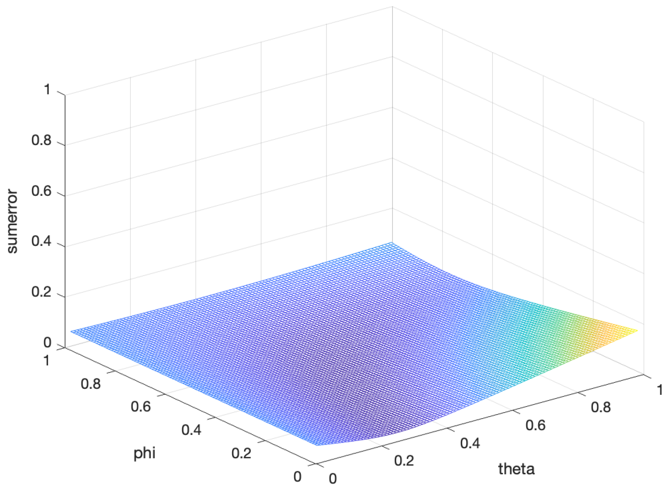
Figure 1. The sum of the error of five-fold cross-validation between the proposed estimation and the population covariance matrix under the different θ and ϕ for N = 100 .
Mathematics 10 04282 g001
Figure 2. Thesum of the error of the five-fold cross-validation between the proposed estimation and the population covariance matrix under the different θ and ϕ for N = 200 .
Mathematics 10 04282 g002
Figure 3. The sum of the error of the five-fold cross-validation between the proposed estimation and the population covariance matrix under the different θ and ϕ for N = 400 .
Mathematics 10 04282 g003
Figure 4. The mean return of the out-of-sample data for N = 100 .
Mathematics 10 04282 g004
Figure 5. The mean return of the out-of-sample data range from the 101st asset to the 200th asset.
Mathematics 10 04282 g005
Figure 6. The mean return of the out-of-sample data range from the 201st asset to the 400th asset.
Mathematics 10 04282 g006
Figure 7. The assets’ weights of each estimation under the out-of-sample data N = 200 .
Mathematics 10 04282 g007
Figure 8. The assets’ weights of each estimation under the out-of-sample data for N = 400 .
Mathematics 10 04282 g008
Figure 9. The assets’ weights of the identity matrix under the out-of-sample data N = 400 .
Mathematics 10 04282 g009
Table 1. The related literature review.
AuthorBrief IntroductionRef.
Ledoit, O., Wolf, M.Under the assumption of the large dimension asymptotic, Ledoit and Wolf kept the eigenvectors of the sample covariance matrix and shrunk the inverse sample eigenvalues to construct a rotation-invariant estimator of the large covariance matrix.[34]
Donoho et al.Based on spiked covariance and the rotation-invariant estimator, Donoho et al. demonstrated that the optimal estimation of the population covariance matrix is related to the best shrinker, which acts as an element of the sample eigenvalues.[35]
J. Bun et al.J. Bun et al. established the asymptotic global law estimate model for three general classes of noisy matrices using the replica method and introduced how to “clean” the noisy eigenvalues of the noisy observation matrix.[36]
Debashis Paul, Alexander AueDebashis Paul and Alexander Aue summarized the random matrix theory (RMT) and described how the development of high-dimensional statistical inference theory and practice is affected by the corresponding development in the RMT field.[37]
Table 2. The estimators for comparison.
The Formulation of EstimationRef.
Σ S C M = 1 N 1 i = 1 N ( r i μ ) ( r i μ ) [42]
Σ I d e n t i t y = I [8,38]
Σ L = ρ ^ Σ S C M + ( 1 ρ ^ ) Σ F [13]
Σ N L = U N D N o r U N * , λ i o r = λ i | 1 c c λ i m ˘ F ( λ i ) | [15,18,43]
Σ D = ϕ ( θ Σ F + ( 1 θ ) Σ M P ) + ( 1 ϕ ) Σ S C M [33]
Σ * = ϕ ( θ Σ F + ( 1 θ ) Σ R I E ) + ( 1 ϕ ) Σ S C M /
Table 3. The optimal parameters θ and ϕ in convex combination and the sum of the corresponding error.
N θ ϕ Error
1000.33330.36360.0273
2000.34340.39390.0515
4000.39390.40400.1080
Table 4. The error between each estimator and the population covariance matrix under the optimal parameter.
N Σ SCM Σ Identity Σ L Σ NL Σ D Σ *
1000.01329.99270.01210.01280.01170.0055
2000.029114.13130.02610.02820.02560.0103
4000.058019.98420.05080.05600.04980.0216
Table 5. The variance comparison of six estimations in the minimum variance portfolio.
N Σ SCM Σ Identity Σ L Σ NL Σ D Σ *
1000.00110.96940.00110.00108.0298 *7.0942 *
2007.8576 *0.39567.9096 *7.7615 *6.7529 *5.9007 *
4003.8828 *0.10774.2676 *3.8435 *3.7395 *3.1368 *
* denotes the unit is 10−4.
Table 6. The out-of-sample performance comparison between each estimator of the 41 assets in SSE50.
IndexAverage Return *Standard Deviation *Sharpe Ratio
Σ S C M 50.4027.981.7390
Σ I d e n t i t y 50.4027.531.7399
Σ L 50.4028.001.7375
Σ N L 50.4027.951.7400
Σ D 50.4027.962.7399
Σ * 50.4027.971.7391
* denotes the unit is %.
Table 7. The out-of-sample performance comparison between each estimations of the 218 assets in HS300.
IndexAverage Return *Standard Deviation *Sharpe Ratio
Σ S C M 50.4018.692.6031
Σ I d e n t i t y 50.4020.282.3990
Σ L 50.4018.702.6017
Σ N L 50.4017.792.7340
Σ D 50.4017.812.7314
Σ * 50.4018.682.6044
* denotes the unit is %.
Table 8. The out-of-sample performance comparison between each estimations of the 426 assets in CSI500.
IndexAverage Return *Standard Deviation *Sharpe Ratio
Σ S C M 50.4021.252.2899
Σ I d e n t i t y 50.4023.042.1115
Σ L 50.4021.242.2909
Σ N L 50.4021.222.2927
Σ D 50.4021.182.2970
Σ * 50.4020.872.3315
* denotes the unit is %.
Table 9. The difference in the out-of-sample variance between Σ * and the alternative estimation with all assets (the significance level is 5 % ).
Number of Assets Σ SCM Σ Identity Σ L Σ NL Σ D
41−0.00010.0350−0.00190.00110.0010
218−0.0000−0.1607−0.00100.09860.0966
426−0.0363−0.1979−0.0350−0.0342−0.0303
Publisher’s Note: MDPI stays neutral with regard to jurisdictional claims in published maps and institutional affiliations.