Bifurcation and Multiplicity of Solutions of the Navier–Stokes Equations in Driven Semi-Elliptical Cavity Flow

Abstract

In this paper, bifurcations in the solution of the Navier–Stokes equations are studied and multiple solutions of the driven semi-elliptical cavity flow are presented. The two-dimensional steady incompressible driven viscous flow in a semi-elliptical cavity is solved numerically. To this end, the problem is formulated using an elliptic coordinate system that transforms the geometry conformally and provides a body fitted coordinate system. The presented results show that above a bifurcation Reynolds number the solution of the governing flow equations bifurcates and there exist multiple solutions for a particular Reynolds number when the aspect ratio of the semi-elliptical cavity geometry is 0.26 ⩽D⩽ 0.8. The bifurcation Reynolds numbers for different aspect ratios and also multiple solutions at different Reynolds numbers are presented in detail.

1. Introduction

The governing Navier–Stokes equations in fluid mechanics are the nonlinear systems of equations and they can possess more than one solution by nature [1,2]. The non-uniqueness of solutions of the Navier–Stokes Equations is primarily due to the nonlinearity of the differential equations, or variation of geometric or fluid mechanical parameters [1]. Finding and dealing with flow problems that have multiple solutions is a challenging and arduous task. These flow problems with multiple solutions exhibit interesting flow features; therefore, they are interesting and intriguing for applied mathematicians and fluid dynamics researchers.

In the literature, there are some studies that present particular fluid flow problems that have multiple solutions at a given Reynolds number. As an example of such flow problems that have multiple solutions, Lemée et al. [3] and Prasad et al. [4] presented multiple solutions to square cavity flow driven by two opposite-facing walls. Similarly, Wahba [5] and Perumal et al. [6] presented multiple solutions of square cavity flow driven by two non-facing walls. Moreover, Zhuo et al. [7], Wahba [5] and Perumal et al. [6] presented multiple solutions of square cavity flow driven by four side walls. These studies are examples for flow problems with square cavity geometry that has multiple solutions.

As an example of different geometry flow problems, Albensoeder et al. [8] studied the rectangular cavity flow driven by two facing side walls using the finite volume method. Their [8] results showed that the solution of two-dimensional steady incompressible flow in a rectangular cavity has several bifurcations and they [8] have presented different non-unique solutions of rectangular cavity flow for different aspect ratios. Chen et al. [9] also studied the two-sided driven rectangular cavity flow and presented multiple solutions.

We note that these flow problems, i.e., the square cavity flow driven by two opposite-facing walls [3,4] or driven by two non-facing walls [5,6] or driven by four side walls [7], have mirror symmetry in geometry and also in boundary conditions. The same is true for the rectangular geometry flow problem which is driven by two facing side walls also. In these flow problems, it is possible to draw a mirror symmetry line such that across this line the geometry and also boundary conditions have mirror symmetry. Although these flow problems have mirror symmetry by definition, the multiple solutions can exhibit mirror symmetric and non-symmetric behavior [8].

Unlike the mirror-symmetric flow problems mentioned above, Erturk [10] has presented multiple solutions for arc-shaped cavity flow. The arc-shaped cavity flow problem, by definition, does not have a mirror-symmetry line. Erturk [10] showed that above a bifurcation Reynolds number, the driven flow in an arc-shaped cavity with an arc length ratio less than 1/2, has two different multiplicity solutions at a given particular Reynolds number. Erturk [10] presented bifurcation Reynolds numbers for arc-shaped cavity geometry with different arc length ratios and also presented multiple solutions of arc-shaped cavity flow at various Reynolds numbers.

The driven semi-elliptical cavity flow problem looks very similar to the driven arc-shaped cavity flow problem considered by Erturk [10] in terms of the geometry with a straight moving lid at the top together with a non-moving stationary curved bottom wall at the bottom.

In the literature, to the best of our knowledge, there are only two studies that consider the flow in a semi-elliptical cavity with an aspect ratio less than unity ($D<1$). Idris et al. [11] studied the lid-driven cavity flow inside a semi-ellipse shallow cavity using a non-uniform mesh. They [11] considered three different aspect ratios (1:4, 1:3 and 3:8) for the semi-ellipse geometry and presented solutions for a range of Reynolds numbers between $Re=100$ and $Re=2000$. Ren and Guo [12] studied the steady flow in a two-dimensional lid-driven semi-elliptical cavity using the lattice Boltzmann simulation method. They [12] considered a wide range of aspect ratios for the elliptic cavity with values less and also greater than unity ($0.1\le D\le 4$). They presented detailed solutions of steady flow in a semi-elliptical cavity up to $Re=5000$. Aside from these two studies [11,12], the flow in a semi-elliptical cavity is not completely understood, especially in terms of bifurcation of the solution at high Reynolds numbers and this constitutes the main motivation of the present study.

At high Reynolds numbers (high inertial forces, i.e., high velocity, with respect to small viscous forces, i.e., very small viscosity) stationary flow loses stability and undergoes transition to turbulence eventually [13]. By nature, turbulence is three-dimensional and unsteady. Along with transient solutions, stationary steady solutions of Navier–Stokes equations still exists at high Reynolds number regimes. For the theory of the Navier–Stokes model, it is important to study the stationary solution at high Reynolds numbers even when the flow loses stability [14,15,16].

The aim of this study is then to solve the semi-elliptical cavity flow numerically, especially at high Reynolds numbers and present bifurcation Reynolds number and also present multiple solutions of the Navier–Stokes equations as the Reynolds number increases for different aspect ratios of the elliptic cavity geometry. In Section 2, the numerical simulation details are given. Comparison of the numerical solutions with the available solutions found in the literature, discussions of the bifurcation and detailed multiple solutions of the semi-elliptical cavity flow are presented in Section 3. Finally, in Section 4, the conclusions are presented.

2. Numerical Method

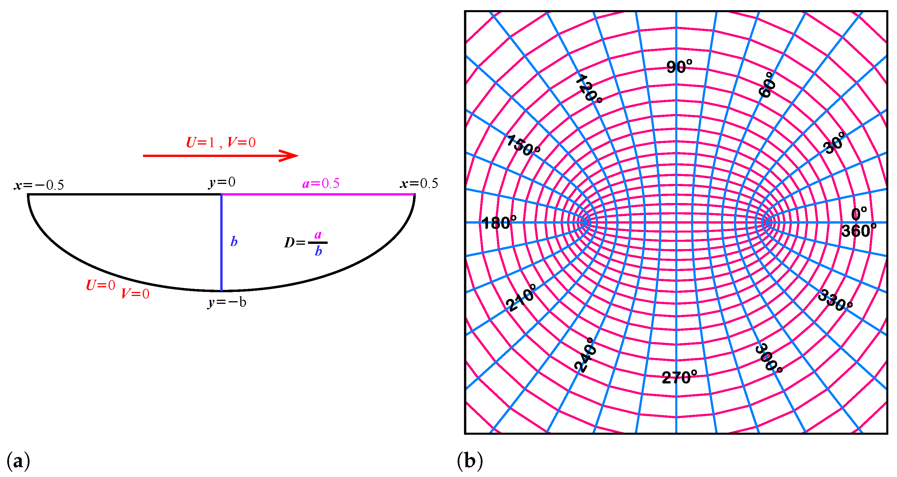
The schematic and the geometry of the driven semi-elliptical cavity flow problem is given in Figure 1a. The top wall of the semi-elliptical cavity is moving while the curved bottom wall is stationary. The incompressible two-dimensional viscous flow inside the driven semi-elliptical cavity is governed by the Navier–Stokes equation and we consider the streamfunction and vorticity formulation of the Navier–Stokes equation as the following

$$\frac{{\partial }^2\psi }{\partial x^2}+\frac{{\partial }^2\psi }{\partial y^2}=-\omega$$

(1)

$$\frac{\partial \psi }{\partial y}\frac{\partial \omega }{\partial x}-\frac{\partial \psi }{\partial x}\frac{\partial \omega }{\partial y}=\frac{1}{Re}\left(\frac{{\partial }^2\omega }{\partial x^2}+\frac{{\partial }^2\omega }{\partial y^2}\right)$$

(2)

where $Re$ is the Reynolds number based on the top wall velocity (U) and the width of the top wall (L) which are both equal to unity.

By nature, the geometry of the semi-elliptical cavity flow problem suggests that the problem is best solved by using an elliptic coordinate system since the elliptic coordinate system transforms the geometry conformally and automatically generate a body fitted coordinate system. The elliptic coordinate system consists of confocal ellipses and hyperbolae, as shown in Figure 1b. The transformation from elliptic coordinates ($\xi ,\eta$) to the Cartesian ($x,y$) coordinates is given by

$$x+iy=ccosh\left(\xi +i\eta \right)$$

(3)

where i is the imaginary number, the elliptic coordinates $\xi \ge 0$ and $0\le \eta \le 2\pi$ and also c is the elliptical eccentricity such that

$$c=\sqrt{a^2-b^2}$$

(4)

and a and b denote the semi-major and semi-minor axes of the ellipse as shown in Figure 1a. In our case, the length of the top wall of the ellipse is equal to unity such that $a=0.5$. Different ellipses are defined by the vertical-to-horizontal semi-axis ratio, i.e., the aspect ratio (D), defined as the following

$$D=\frac{b}{a}$$

(5)

The Cartesian coordinates can be defined in terms of elliptic coordinates as the following

$$x=ccosh\xi cos\eta$$

(6)

$$y=csinh\xi sin\eta$$

(7)

Using the elliptic coordinate transformation (3), the streamfunction and vorticity equations in elliptic coordinates are given by

$$\frac{{\partial }^2\psi }{\partial {\xi }^2}+\frac{{\partial }^2\psi }{\partial {\eta }^2}=-J\omega$$

(8)

$$\frac{\partial \psi }{\partial \eta }\frac{\partial \omega }{\partial \xi }-\frac{\partial \psi }{\partial \xi }\frac{\partial \omega }{\partial \eta }=\frac{1}{Re}\left(\frac{{\partial }^2\omega }{\partial {\xi }^2}+\frac{{\partial }^2\omega }{\partial {\eta }^2}\right)$$

(9)

where J denotes the Jacobian of the transformation and it is defined as the following

$$J=\frac{\partial x}{\partial \xi }\frac{\partial y}{\partial \eta }-\frac{\partial x}{\partial \eta }\frac{\partial y}{\partial \xi }$$

(10)

We note that the governing equations of the driven semi-elliptical cavity flow are nonlinear ((8) and (9)); therefore, they are solved in an iterative manner. For this, we assign pseudo time derivatives to the governing equations as the following

$$\frac{\partial \psi }{\partial t}=\frac{{\partial }^2\psi }{\partial {\xi }^2}+\frac{{\partial }^2\psi }{\partial {\eta }^2}+J\omega$$

(11)

$$\frac{\partial \omega }{\partial t}=\frac{1}{Re}\left(\frac{{\partial }^2\omega }{\partial {\xi }^2}+\frac{{\partial }^2\omega }{\partial {\eta }^2}\right)-\frac{\partial \psi }{\partial \eta }\frac{\partial \omega }{\partial \xi }+\frac{\partial \psi }{\partial \xi }\frac{\partial \omega }{\partial \eta }$$

(12)

and then solve these equations through the pseudo time until steady state solution (i.e., $\frac{\partial \psi }{\partial t}\approx \frac{\partial \omega }{\partial t}\approx 0$) is obtained. We use the ADI (Alternating Implicit Direction) method in order to advance the above equations in the pseudo time. The ADI method involves a two step iteration process. In the first step, using the following implicit system, the solution is advanced to intermediate half time level by using a tri-diagonal solver.

$$\frac{{\psi }^{n+\frac{1}{2}}-{\psi }^n}{\frac{\Delta t}{2}}={\frac{{\partial }^2\psi }{\partial {\xi }^2}}^{n+\frac{1}{2}}+{\frac{{\partial }^2\psi }{\partial {\eta }^2}}^n+J{\omega }^n$$

(13)

$$\frac{{\omega }^{n+\frac{1}{2}}-{\omega }^n}{\frac{\Delta t}{2}}=\frac{1}{Re}{\frac{{\partial }^2\omega }{\partial {\xi }^2}}^{n+\frac{1}{2}}+\frac{1}{Re}{\frac{{\partial }^2\omega }{\partial {\eta }^2}}^n-{\frac{\partial \psi }{\partial \eta }}^n{\frac{\partial \omega }{\partial \xi }}^{n+\frac{1}{2}}+{\frac{\partial \psi }{\partial \xi }}^n{\frac{\partial \omega }{\partial \eta }}^n$$

(14)

Here, the superscript denotes the pseudo time level. After obtaining the solution at the intermediate half time level (i.e., ${\psi }^{n+\frac{1}{2}}$ and ${\omega }^{n+\frac{1}{2}}$), in the second step, using the following implicit system, the solution is advanced to a new time level (i.e., ${\psi }^{n+1}$ and ${\omega }^{n+1}$) again using a tri-diagonal solver.

$$\frac{{\psi }^{n+1}-{\psi }^{n+\frac{1}{2}}}{\frac{\Delta t}{2}}={\frac{{\partial }^2\psi }{\partial {\xi }^2}}^{n+\frac{1}{2}}+{\frac{{\partial }^2\psi }{\partial {\eta }^2}}^{n+1}+J{\omega }^{n+\frac{1}{2}}$$

(15)

$$\frac{{\omega }^{n+1}-{\omega }^{n+\frac{1}{2}}}{\frac{\Delta t}{2}}=\frac{1}{Re}{\frac{{\partial }^2\omega }{\partial {\xi }^2}}^{n+\frac{1}{2}}+\frac{1}{Re}{\frac{{\partial }^2\omega }{\partial {\eta }^2}}^{n+1}-{\frac{\partial \psi }{\partial \eta }}^{n+\frac{1}{2}}{\frac{\partial \omega }{\partial \xi }}^{n+\frac{1}{2}}+{\frac{\partial \psi }{\partial \xi }}^{n+\frac{1}{2}}{\frac{\partial \omega }{\partial \eta }}^{n+1}$$

(16)

We note that in order to start the iteration process we assign initially guessed values to the variables (i.e., ${\psi }^0$, ${\omega }^0$) and then using the ADI method as described above advance the solution in the pseudo time.

Using the chain rule, in elliptic coordinate system the U and V velocities in x- and y-directions are defined as the following

$$U=\frac{\partial \psi }{\partial y}=\frac{\partial \psi }{\partial \xi }\frac{\partial \xi }{\partial y}+\frac{\partial \psi }{\partial \eta }\frac{\partial \eta }{\partial y}$$

$$V=-\frac{\partial \psi }{\partial x}=-\frac{\partial \psi }{\partial \xi }\frac{\partial \xi }{\partial x}-\frac{\partial \psi }{\partial \eta }\frac{\partial \eta }{\partial x}$$

(17)

The no-slip no-penetration boundary conditions state that on the top moving wall the fluid velocities are U = 1 and V = 0 and on the curved bottom wall they are U = 0 and V = 0, as shown in Figure 1a. These boundary conditions state that on the wall the value of the streamfunction is zero (i.e., $\psi$ = 0). Using the streamfunction Equation (8) and also Equation (17), the value of the vorticity on the wall is calculated as the following

$${\omega }_0=\frac{1}{J}\frac{-2{\psi }_1}{\Delta {\eta }^2}+\frac{1}{J}\frac{2U}{\Delta \eta \frac{\partial \eta }{\partial y}}$$

(18)

where subscript 0 refers to wall grid points, 1 refers to adjacent grid points next to the wall, $\Delta \eta$ refers to grid spacing and U refers to wall velocity such that it is equal to 1 on the top moving wall and 0 on the stationary curved bottom wall.

During the numerical iterations, the following residuals are monitored at each pseudo time step

$$Residua{l}_{\psi }=max\left(\left|\frac{{\psi }_{i,j}^{n+1}-{\psi }_{i,j}^n}{{\psi }_{i,j}^n}\right|\right)$$

$$Residua{l}_{\omega }=max\left(\left|\frac{{\omega }_{i,j}^{n+1}-{\omega }_{i,j}^n}{{\omega }_{i,j}^n}\right|\right)$$

(19)

where subscripts show the grid index and max denote the maximum absolute value in the whole computational domain. By definition, these residuals show the change in the streamfunction and vorticity variables between two consecutive pseudo time steps normalized by the streamfunction and vorticity value at the previous pseudo time step. In the present study we continue the iterations until both $Residua{l}_{\psi }$ and $Residua{l}_{\omega }$ are less than ${10}^{-10}$, which means that at the convergence the streamfunction and vorticity values change only 0.00000001% between two iteration steps at a grid point as the maximum and even less in the other grid points in the computational domain. This convergence criterion is used for every multiple solution presented in the current study.

The numerical algorithm followed in the present study is given schematically in Figure 2.

3. Results and Discussions

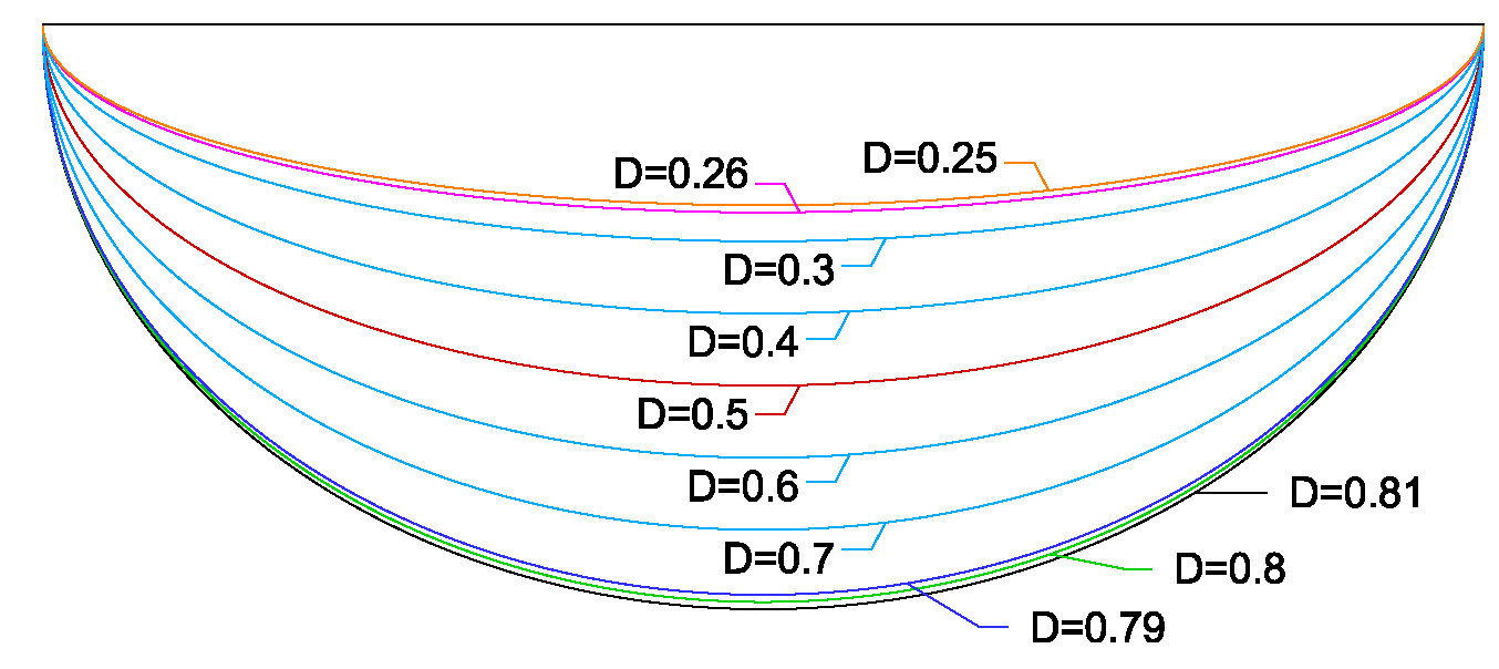
Figure 3 shows semi-elliptical cavity geometries that are considered in the present study. In the present study, numerical solutions of driven semi-elliptical cavity flow with aspect ratios (D) of 0.26, 0.5 and 0.8 will be presented in detail even though many more aspect ratios are considered. In all of the considered aspect ratio ellipses, first grid refined studies are carried out such that all of the solutions presented here are grid independent solutions.

First, we compare our numerical solutions with those of Idris et al. [11] and Ren and Guo [12] and consider the same semi-ellipse cases and Reynolds numbers. Idris et al. [11] considered aspect ratios of 1:4, 1:3 and 3:8 in their study. Their definition of aspect ratio corresponds to $D=0.5$, 0.6667 (2/3) and 0.75, respectively, with the definition used in the present study. For these aspect ratios, Idris et al. [11] present numerical data for minimum and also maximum streamfunction values at the primary and secondary vortex centers and the (x,y) location of the these centers for $Re=100$, 500, 1000, 1500 and 2000.

Table 1. Comparison of flow properties for $D=0.5$, 0.6667 and 0.75 aspect ratio semi-ellipses.

D			Re = 100	Re = 500	Re = 1000	Re = 1500	Re = 2000
0.5	Present Study	${\psi }_{min}$	−0.03656	−0.03819	−0.04069	−0.04018	−0.03917
		$(x,y)$	(0.5507, 0.1679)	(0.7300, 0.1661)	(0.7429, 0.1603)	(0.7587, 0.1610)	(0.7759, 0.1623)
		${\psi }_{max}$	-	-	-	0.00089	0.00206
		$(x,y)$				(0.5050, 0.0583)	(0.5000, 0.0770)
	Idris et al. [11]	${\psi }_{min}$	−0.03650	−0.03803	−0.04055	−0.03983	−0.03858
		$(x,y)$	(0.5490, 0.1658)	(0.7357, 0.1658)	(0.7464, 0.1600)	(0.7464, 0.1600)	(0.7879, 0.1658)
		${\psi }_{max}$	-	-	-	0.00096	0.00213
		$(x,y)$				(0.5123, 0.0567)	(0.5123, 0.0777)
0.6667	Present Study	${\psi }_{min}$	−0.04827	−0.05291	−0.05335	−0.05208	−0.05078
		$(x,y)$	(0.5849, −0.1089)	(0.7100, −0.1199)	(0.7094, −0.1258)	(0.7275, −0.1234)	(0.7433, −0.1210)
		${\psi }_{max}$	-	-	0.00076	0.00283	0.00405
		$(x,y)$			(0.3733, −0.2490)	(0.3625, −0.2053)	(0.3265, −0.1894)
	Idris et al. [11]	${\psi }_{min}$	−0.04811	−0.05257	−0.05291	−0.05133	−0.05005
		$(x,y)$	(0.5855, −0.2288)	(0.7138, −0.1200)	(0.7138, −0.1276)	(0.7357, −0.1200)	(0.7571, −0.1200)
		${\psi }_{max}$	-	-	0.00082	0.00301	0.00505
		$(x,y)$			(0.3786, −0.0864)	(0.3666, −0.2051)	(0.3201, −0.1919)
0.75	Present Study	${\psi }_{min}$	−0.05396	−0.05941	−0.05950	−0.05820	−0.05690
		$(x,y)$	(0.5970, −0.1215)	(0.6925, −0.1385)	(0.6906, −0.1444)	(0.7080, −0.1429)	(0.7213, −0.1404)
		${\psi }_{max}$	-	-	0.00119	0.00341	0.00472
		$(x,y)$			(0.3101, −0.2491)	(0.3019, −0.2077)	(0.2791, −0.1915)
	Idris et al. [11]	${\psi }_{min}$	−0.05376	−0.05888	−0.05874	−0.05716	−0.05538
		$(x,y)$	(0.5975, −0.1176)	(0.6913, −0.1350)	(0.6913, −0.1435)	(0.7138, −0.1435)	(0.7357, −0.1350)
		${\psi }_{max}$	-	-	0.00126	0.00379	0.00505
		$(x,y)$			(0.3201, −0.2518)	(0.3087, −0.2083)	(0.2862, −0.1928)

tabulates present results at the same Reynolds numbers along with those from Idris et al. [11].

In their study, Ren and Guo [12] also considered aspect ratios of $D=0.25$ and 0.5 for Reynolds number of $Re=$ 500, 1000, 3000 and 5000.

Table 2. Comparison of flow properties for $D=0.25$ and 0.5 aspect ratio semi-ellipses.

D			Re = 500	Re = 1000	Re = 3000	Re = 5000
0.25	Present Study	${\psi }_{min}$	−0.0184	−0.0183	−0.0202	−0.0199
		$(x,y)$	(0.5660, 0.0833)	(0.6307, 0.0845)	(0.7986, 0.0819)	(0.8298, 0.0849)
		${\psi }_{max}$	-	-	-	4.9552 $\times {10}^{-4}$
		$(x,y)$				(0.7107, 0.0326)
	Ren and Guo [12]	${\psi }_{min}$	−0.0182	−0.0181	−0.0200	−0.0197
		$(x,y)$	(0.5640, 0.0835)	(0.6294, 0.0840)	(0.7979, 0.0825)	(0.8296, 0.0845)
		${\psi }_{max}$	-	-	-	4.6623 $\times {10}^{-4}$
		$(x,y)$				(0.7119, 0.0332)
0.5	Present Study	${\psi }_{min}$	−0.03819	−0.04069	−0.03708	−0.03410
		$(x,y)$	(0.7300, 0.1661)	(0.7429, 0.1603)	(0.8048, 0.1667)	(0.8347, 0.1729)
		${\psi }_{max}$	-	-	0.003400	0.005116
		$(x,y)$			(0.3970, 0.0950)	(0.2639, 0.1175)
	Ren and Guo [12]	${\psi }_{min}$	−0.0376	−0.0401	−0.0365	−0.0335
		$(x,y)$	(0.7295, 0.1670)	(0.7441, 0.1602)	(0.8047, 0.1670)	(0.8350, 0.1729)
		${\psi }_{max}$	-	-	0.0033	0.0050
		$(x,y)$			(0.4033, 0.0938)	(0.2676, 0.1172)

tabulates present data for the same cases in comparison with those of Ren and Guo [12].

Both Table 1 and Table 2 show that our numerical results are in very good agreement with those of Idris et al. [11] and Ren and Guo [12], although we believe that our results are more accurate due to the body fitted fine mesh used in the numerical simulation together with the very low residuals considered for the convergence.

In a study, Erturk [10] considered the flow inside a driven arc-shaped cavity and reported that when the arc length ratio is less than 1/2, above a bifurcation Reynolds number the arc-shaped cavity flow has multiple solutions for a given particular Reynolds number. Erturk [10] finds that below a bifurcation Reynolds number, a single solution exists for the governing Navier–Stokes equations for the arc-shaped cavity flow; however, above the bifurcation Reynolds number, two different solutions exist for a given particular Reynolds number. Erturk [10] also finds that this bifurcation Reynolds number varies as the arc length ratio changes. For arc-shaped cavity geometries with various arc length ratios, Erturk [10] presented the bifurcation Reynolds number at which multiple solutions start to exist and also presented the two different solutions of the Navier–Stokes equations at various Reynolds numbers above the bifurcation Reynolds number. Erturk [10] called the only solution that exists below the bifurcation Reynolds number the “1st solution” and also the new solution that starts to exist above the bifurcation Reynolds number the “2nd solution”. In order to obtain the “1st solution” and also the “2nd solution”, Erturk [10] made the following statements:

• Below the bifurcation Reynolds number, if the homogeneous solution is used as an initial guess for the iterations, the obtained solution is the 1st solution.
• Above the bifurcation Reynolds number, if the homogeneous solution is used as an initial guess for the iterations, the solution always converges to the 2nd solution.
• Below the bifurcation Reynolds number, the 2nd solution does not exist. The 2nd solution exists only above the bifurcation Reynolds number.
• If the 1st solution with previous smaller Reynolds number is used as an initial guess for the iterations, it is possible to obtain the 1st solution even above the bifurcation Reynolds number. The 1st solution exists above the bifurcation Reynolds number.

In the present study, we use the same classification used in Erturk [10] and name the only solution “1st solution” when the Reynolds number is below the bifurcation Reynolds number and also name the new solution that starts to appear above the bifurcation Reynolds number “2nd solution”. In order to obtain the bifurcation Reynolds number and also the multiple solutions of the flow problem we follow the procedure given by Erturk [10].

First, we start with a semi-ellipse with $D=0.5$ aspect ratio. In order to obtain the bifurcation Reynolds number whereby the governing flow equations start to have multiple solutions, we solve the flow problem at incrementally increasing Reynolds numbers using the homogeneous initial guess for the numerical iterations. Figure 4 shows the streamfunction contours of the solutions obtained at $Re=5058$ and also at $Re=5059$ when homogeneous initial guess is used for the considered aspect ratio ellipse ($D=0.5$). One can see that when the Reynolds number is incremented only by “1”, the vortex structure of the flow and the solution of the governing equations change dramatically. For $D=0.5$ aspect ratio semi-ellipse, the bifurcation Reynolds number is $Re=5059$ and starting from this Reynolds number and above a second solution starts to exist at any considered Reynolds number. We note that we considered only integer $Re$ values.

Below the bifurcation Reynolds number, only one solution exists for the governing flow equations, i.e., the 1st solution, even if different initial guesses are used for the iterations. Figure 5 shows the evolution of the 1st solution at various Reynolds numbers below the bifurcation Reynolds number of $Re=5059$.

In order to obtain the 1st solution above the bifurcation Reynolds number, for example, at $Re=6000$, we use the 1st solution at $Re=5058$ as initial guess for the iterations. The obtained 1st solution at $Re=6000$ is given in Figure 6a. In order to obtain the 2nd solution above the bifurcation Reynolds number, for example, at $Re=6000$, we use the 2nd solution at $Re=5059$ as initial guess for the iterations. The obtained 2nd solution at $Re=6000$ is given in Figure 6b. Then, using the corresponding 1st or 2nd solutions at previous smaller Reynolds numbers, we solve for the 1st or 2nd solutions at higher Reynolds numbers. We note that we advance the Reynolds number by incrementing 1000. Using the previous 1st solution at smaller Reynolds number as initial guess for the next higher Reynolds number, we were able to obtain the 1st solution until $Re=$ 14,000 at maximum. Moreover, using the previous 2nd solution at smaller Reynolds number as initial guess for the next higher Reynolds number, we were able to obtain the 2nd solution until $Re=$ 30,000 at maximum. 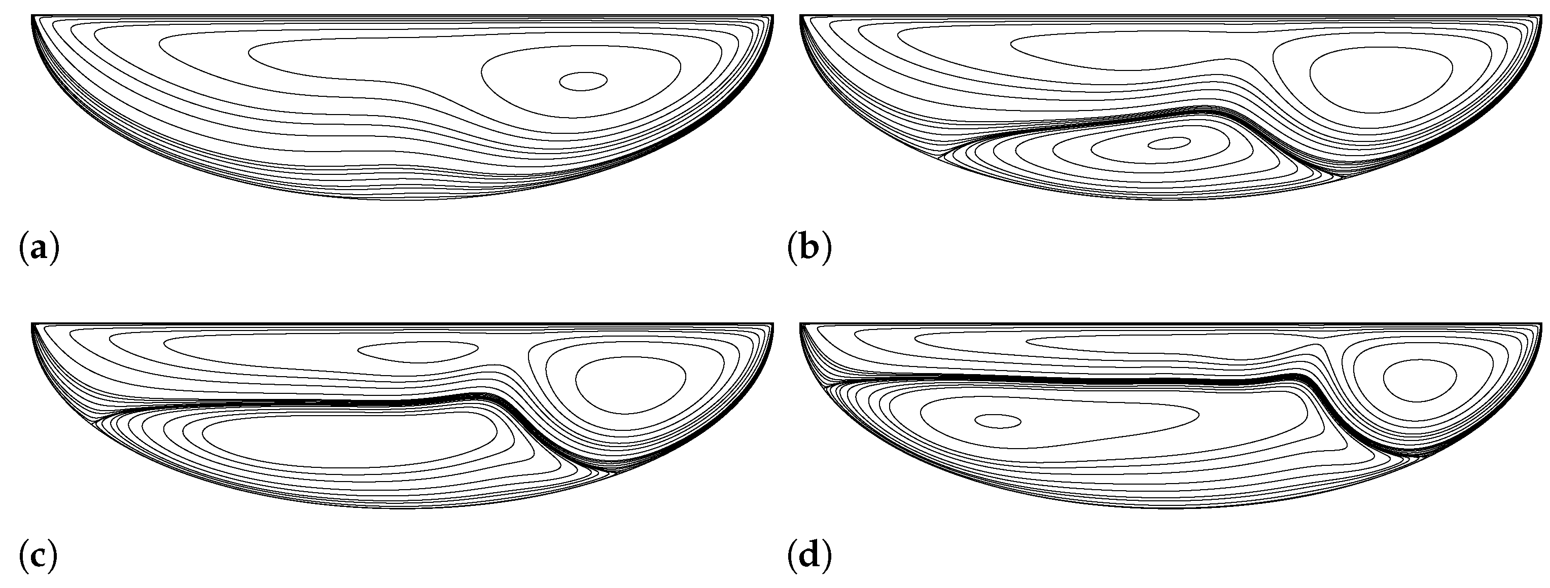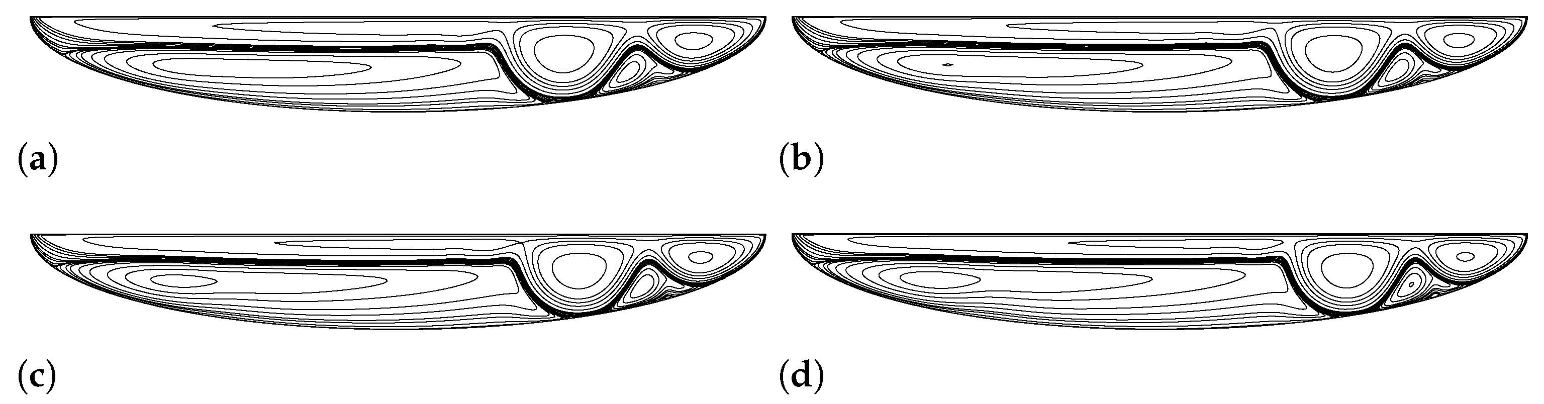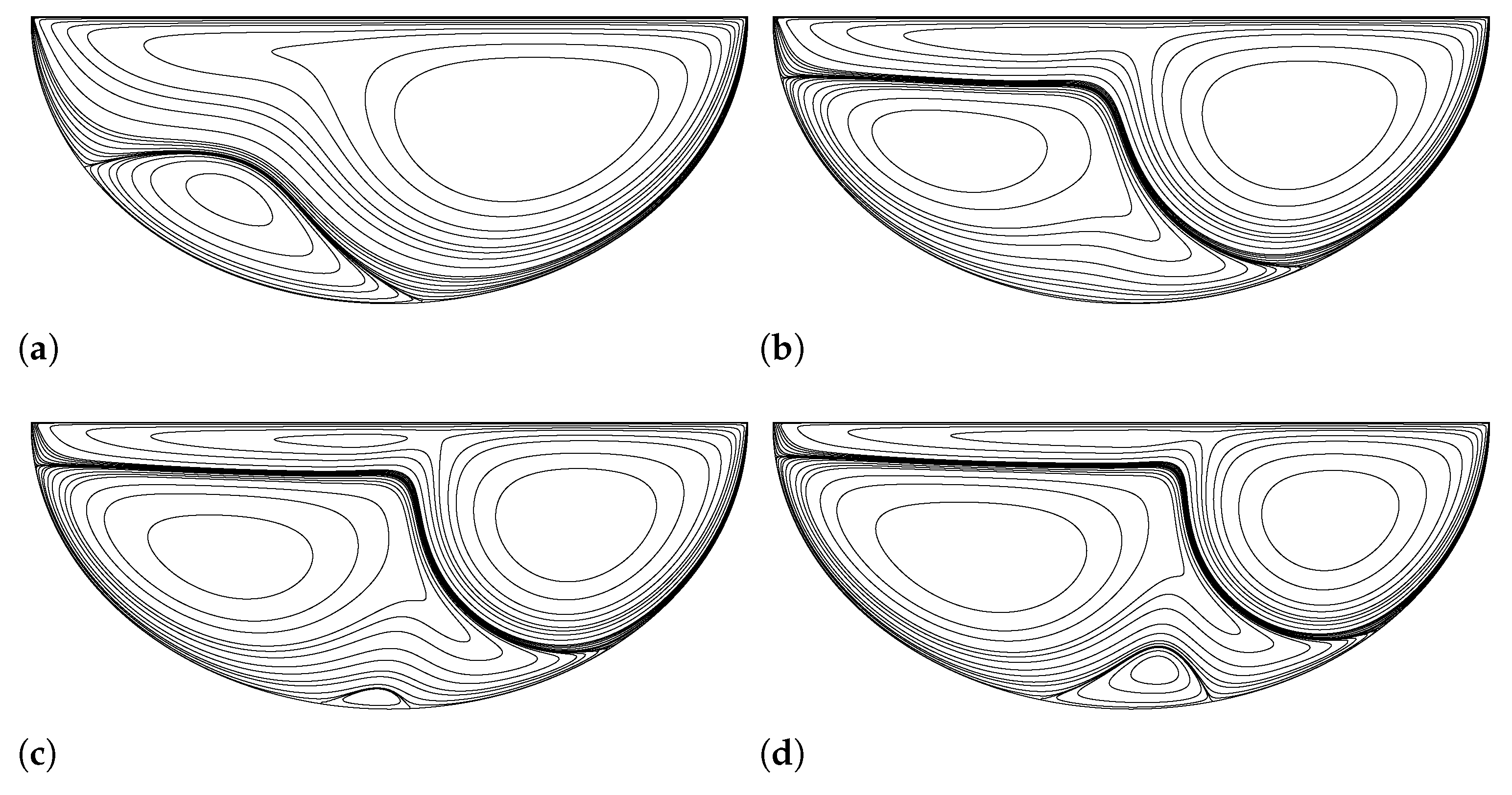Figure 6 shows the streamfunction contours of both the 1st and 2nd solutions at various same Reynolds numbers until $Re=$ 14,000, i.e., until the maximum Reynolds number for the 1st solution. Above $Re=$ 14,000, only the 2nd solution exists and Figure 7 shows the streamfunction contours of the 2nd solution at various Reynolds numbers until $Re=$ 30,000.

For future references, for the 1st and 2nd solutions given in Figure 4, Figure 5, Figure 6 and Figure 7 we tabulate the streamfunction ($\psi$) and vorticity ($\omega$) values at the center of the strongest clockwise rotating vortex (i.e., at the location of ${\psi }_{min}$) and also at the center of the strongest counterclockwise rotating vortex (i.e., at the location of ${\psi }_{max}$) together with the x-y locations of these centers for the 1st solution in

Table 3. Minimum and maximum streamfunction values in the 1st solution, corresponding vorticity values and (x,y) locations for $D=0.5$ aspect ratio.

	$\mathit{Re}$	$\mathit{\psi }$	$\mathit{\omega }$	x	y
${\psi }_{min}$	1000	−4.0692 $\times {10}^{-2}$	−10.4608	0.2429	−0.0898
	2000	−3.9172 $\times {10}^{-2}$	−11.4166	0.2759	−0.0877
	3000	−3.7078 $\times {10}^{-2}$	−12.3001	0.3048	−0.0833
	5000	−3.4102 $\times {10}^{-2}$	−13.5900	0.3347	−0.0771
	5058	−3.4034 $\times {10}^{-2}$	−13.6213	0.3347	−0.0771
	6000	−3.3017 $\times {10}^{-2}$	−14.0960	0.3439	−0.0744
	10,000	−2.9954 $\times {10}^{-2}$	−15.6555	0.3677	−0.0693
	14,000	−2.7920 $\times {10}^{-2}$	−16.8082	0.3813	−0.0652
${\psi }_{max}$	1000	-	-	-	-
	2000	2.0556 $\times {10}^{-3}$	2.2127	0.0000	−0.1730
	3000	3.3996 $\times {10}^{-3}$	2.5158	−0.1030	−0.1551
	5000	5.1156 $\times {10}^{-3}$	3.0504	−0.2361	−0.1325
	5058	5.1566 $\times {10}^{-3}$	3.0451	−0.2361	−0.1325
	6000	5.7257 $\times {10}^{-3}$	3.1173	−0.2500	−0.1276
	10,000	6.6387 $\times {10}^{-3}$	3.2087	−0.2795	−0.1130
	14,000	6.7587 $\times {10}^{-3}$	3.3534	−0.3047	−0.1046

and the same for the 2nd solution in

Table 4. Minimum and maximum streamfunction values in the 2nd solution, corresponding vorticity values and (x,y) locations for $D=0.5$ aspect ratio.

	$\mathit{Re}$	$\mathit{\psi }$	$\mathit{\omega }$	x	y
${\psi }_{min}$	5059	−3.9349 $\times {10}^{-2}$	−12.5971	0.2996	−0.0845
	6000	−3.8767 $\times {10}^{-2}$	−12.9444	0.3086	−0.0841
	10,000	−3.6024 $\times {10}^{-2}$	−14.2291	0.3351	−0.0786
	14,000	−3.3975 $\times {10}^{-2}$	−15.1813	0.3503	−0.0739
	15,000	−3.3868 $\times {10}^{-2}$	−7.1281	0.0328	−0.1112
	20,000	−3.3634 $\times {10}^{-2}$	−7.2142	0.0631	−0.1126
	25,000	−3.3185 $\times {10}^{-2}$	−7.2723	0.0862	−0.1116
	30,000	−3.2660 $\times {10}^{-2}$	−7.3086	0.1024	−0.1129
${\psi }_{max}$	5059	3.8239 $\times {10}^{-3}$	4.1063	0.0688	−0.1827
	6000	4.2541 $\times {10}^{-3}$	4.2504	0.0979	−0.1806
	10,000	5.0907 $\times {10}^{-3}$	4.9392	0.1681	−0.1680
	14,000	5.3289 $\times {10}^{-3}$	5.5900	0.2045	−0.1641
	15,000	5.3516 $\times {10}^{-3}$	5.7343	0.2111	−0.1629
	20,000	5.3594 $\times {10}^{-3}$	6.3386	0.2375	−0.1594
	25,000	5.2923 $\times {10}^{-3}$	6.8076	0.2564	−0.1549
	30,000	5.1990 $\times {10}^{-3}$	7.1876	0.2712	−0.1530

.

After obtaining the 1st and 2nd solutions of the flow in a driven semi-elliptical cavity with $D=0.5$ aspect ratio, we then extend the analysis for smaller aspect ratios. We first solve the semi-elliptical cavity flow with $D=0.4$ aspect ratio and then solve it for $D=0.3$ aspect ratio by repeating the same procedure we follow for the $D=0.5$ aspect ratio semi-ellipse as described above. For $D=0.4$ and $D=0.3$ aspect ratio semi-elliptical cavity flows, the bifurcation Reynolds numbers are 5546 and 6673, respectively. The $D=0.4$ and $D=0.3$ aspect ratio semi-ellipse cavity geometries are shown in blue color in Figure 3 for comparison with other semi-ellipse geometries. Following this, we then repeat the same analysis for $D=0.25$ aspect ratio semi-elliptical cavity flow. However, for this aspect ratio, we did not observe any bifurcation in the solution as the Reynolds number increases such that there was only one solution for any considered Reynolds number. Multiplicity in the solution does not arise for the $D=0.25$ aspect ratio semi-elliptical cavity flow case. This fact shows that there is a minimum aspect ratio for semi-elliptical cavity flow to have multiplicity in the solution. In order to find this minimum aspect ratio for the semi-elliptical cavity flow to have multiple solutions, we start to solve for different aspect ratio cases incrementing the aspect ratio by 0.01. For any aspect ratio semi-ellipse with $D=0.26$ and above, we find bifurcation in the solution at a certain Reynolds number such that there exists multiplicity in the solution. However, for any aspect ratio semi-ellipse with $D=0.25$ and below, there is no bifurcation in the solution such that only one solution exists for every Reynolds number. Thus, the minimum aspect ratio for the semi-elliptical cavity flow such that multiplicity in the solution exists is $D=0.26$.

For this obtained minimum $D=0.26$ aspect ratio semi-elliptical cavity flow, Figure 8 shows the solution for $Re=7412$ and also for $Re=7413$ when homogeneous initial guess is used for the iterations. As seen in Figure 8a at $Re=7412$ in the 1st solution, there is one counter-rotating vortex just above the curved bottom wall. However, at $Re=7413$ in Figure 8b which is the bifurcation Reynolds number, different than the 1st solution, there are two separate counter-rotating vortices just above the curved bottom wall in the 2nd solution.

Figure 9 shows the evolution of the 1st solution of the driven semi-elliptical cavity flow with $D=0.26$ at various Reynolds numbers below the bifurcation Reynolds number.

For $D=0.26$ aspect ratio semi-ellipse, we were able to advance the 1st solution until a Reynolds number of 16,000. Figure 10 shows both the 1st and 2nd solutions at various same Reynolds numbers until $Re=$ 16,000.

Above $Re=$ 16,000, only the 2nd solution exists for the driven semi-elliptical cavity flow with $D=0.26$ aspect ratio. For this case, we were able to advance the 2nd solution until a Reynolds number of 23,000. Figure 11 shows the 2nd solution at various Reynolds numbers until $Re=$ 23,000 for $D=0.26$ aspect ratio semi-elliptical cavity flow.

Similarly, for future references, for the driven semi-elliptical cavity flow with aspect ratio $D=0.26$, we tabulate the streamfunction ($\psi$) and vorticity ($\omega$) values at the center of the strongest clockwise rotating vortex (i.e., at the location of ${\psi }_{min}$) and also at the center of the strongest counterclockwise rotating vortex (i.e., at the location of ${\psi }_{max}$) together with the x–y locations of these centers for the 1st solution in

Table 5. Minimum and maximum streamfunction values in the 1st solution, corresponding vorticity values and (x,y) locations for $D=0.26$ aspect ratio.

	$\mathit{Re}$	$\mathit{\psi }$	$\mathit{\omega }$	x	y
${\psi }_{min}$	1000	−1.8995 $\times {10}^{-2}$	−16.4531	0.1426	−0.0418
	3000	−2.1097 $\times {10}^{-2}$	−21.9350	0.3000	−0.0446
	5000	−2.0552 $\times {10}^{-2}$	−24.5914	0.3328	−0.0413
	7000	−1.9230 $\times {10}^{-2}$	−27.2741	0.3615	−0.0396
	7412	−1.8899 $\times {10}^{-2}$	−27.8864	0.3682	−0.0387
	8000	−1.8453 $\times {10}^{-2}$	−28.7201	0.3748	−0.0378
	10,000	−1.7224 $\times {10}^{-2}$	−31.1625	0.3920	−0.0351
	13,000	−1.5950 $\times {10}^{-2}$	−34.0247	0.4066	−0.0325
	16,000	−1.5075 $\times {10}^{-2}$	−36.2727	0.4161	−0.0307
${\psi }_{max}$	1000	-	-	-	-
	3000	4.6730 $\times {10}^{-7}$	1.1377	0.1887	−0.1179
	5000	6.4819 $\times {10}^{-4}$	6.7002	0.2079	−0.0939
	7000	1.1217 $\times {10}^{-3}$	8.4353	0.2396	−0.0859
	7412	1.1997 $\times {10}^{-3}$	5.0308	0.0488	−0.0900
	8000	1.4603 $\times {10}^{-3}$	5.5705	0.0590	−0.0872
	10,000	2.1025 $\times {10}^{-3}$	5.9618	−0.0154	−0.0826
	13,000	2.6358 $\times {10}^{-3}$	5.8704	−0.1068	−0.0781
	16,000	3.1678 $\times {10}^{-3}$	6.9743	−0.2315	−0.0728

and the same for the 2nd solution in

Table 6. Minimum and maximum streamfunction values in the 2nd solution, corresponding vorticity values and (x,y) locations for $D=0.26$ aspect ratio.

	$\mathit{Re}$	$\mathit{\psi }$	$\mathit{\omega }$	x	y
${\psi }_{min}$	7413	−1.9781 $\times {10}^{-2}$	−26.6336	0.3546	−0.0406
	8000	−1.9778 $\times {10}^{-2}$	−26.7983	0.3563	−0.0403
	10,000	−1.9138 $\times {10}^{-2}$	−16.5330	0.1693	−0.0507
	13,000	−1.9283 $\times {10}^{-2}$	−16.9627	0.1977	−0.0518
	16,000	−1.9141 $\times {10}^{-2}$	−17.4731	0.2184	−0.0506
	17,000	−1.9065 $\times {10}^{-2}$	−17.6383	0.2252	−0.0502
	19,000	−1.8895 $\times {10}^{-2}$	−17.9560	0.2364	−0.0495
	21,000	−1.8709 $\times {10}^{-2}$	−18.2558	0.2453	−0.0489
	23,000	−1.8517 $\times {10}^{-2}$	−18.5377	0.2542	−0.0505
${\psi }_{max}$	7413	1.1484 $\times {10}^{-3}$	9.4736	0.2331	−0.0890
	8000	1.2202 $\times {10}^{-3}$	9.8365	0.2376	−0.0885
	10,000	1.4310 $\times {10}^{-3}$	11.1247	0.2577	−0.0861
	13,000	1.6593 $\times {10}^{-3}$	11.9499	0.2857	−0.0823
	16,000	1.8258 $\times {10}^{-3}$	11.9386	0.3081	−0.0767
	17,000	1.8698 $\times {10}^{-3}$	12.1282	0.3141	−0.0758
	19,000	2.0018 $\times {10}^{-3}$	5.2195	−0.2900	−0.0666
	21,000	2.1800 $\times {10}^{-3}$	5.3900	−0.2979	−0.0635
	23,000	2.3273 $\times {10}^{-3}$	5.5082	−0.3060	−0.0625

.

Then, we start examining solutions of the semi-elliptical cavity flow with aspect ratios above $D>0.5$. We first solve for $D=0.6$, $D=0.7$ and $D=0.8$ aspect ratio semi-elliptical cavity flows and we obtain the bifurcation Reynolds number for these flows as 5084, 5968 and 7182, respectively. However, for $D=0.9$ aspect ratio, we did not observe any bifurcation in the solution such that there was no multiplicity in the solution as the Reynolds number increases. For this aspect ratio semi-ellipse, we obtain only one solution for any considered Reynolds number. This fact shows that there is a maximum aspect ratio for semi-elliptical cavity flow to have multiplicity in the solution as well. In order to find this maximum aspect ratio such that the flow in a semi-elliptical cavity exhibits multiple solutions, we use the following procedure. First, we choose a high Reynolds number which is above an expected bifurcation Reynolds number, for example, $Re=$ 12,000. We note that for semi-elliptical cavity flow with $D=0.8$ aspect ratio, the bifurcation Reynolds number is 7182; therefore, $Re=$ 12,000 should be well beyond a possible bifurcation. At this high Reynolds number (above bifurcation Reynolds number), i.e., $Re=$ 12,000, when the homogeneous initial guess is used for the iterations, the solution obtained is the 2nd solution as stated by Erturk [10]. We also note that this is true if there is bifurcation in the solution such that the flow has multiple solutions. Using this chosen Reynolds number, we then solve the flow in a semi-elliptical cavity by changing the aspect ratio with 0.01 increments in order to see at which aspect ratio the flow starts to change behavior. Figure 12 shows the solutions we obtain when homogeneous initial guess is used for $Re=$ 12,000 and for $D=0.79$, 0.8, 0.81 and 0.82 aspect ratio semi-elliptical cavity flows. As seen in Figure 12, above $D=0.8$ when the aspect ratio is incremented by only 0.01, i.e., at $D=0.81$, the solution changes dramatically. We note that beyond this aspect ratio ($D>0.8$) the solution resembles the 1st solution. After several numerical experimentations, we did not find any multiplicity in the solution for $D=0.81$ aspect ratio ellipse and above. Thus we find the maximum aspect ratio that the semi-elliptical cavity flow exhibits multiplicity in the solutions as $D=0.8$.

For this obtained maximum $D=0.8$ aspect ratio semi-elliptical cavity flow, Figure 13 shows the solution for $Re=7181$ and also for $Re=7182$ when the homogeneous initial guess is used for the iterations. As seen in Figure 13, for $D=0.8$ aspect ratio semi-ellipse when the Reynolds number is incremented just by 1 from $Re=7181$ to 7182, the flow topology changes dramatically. Thus, for $D=0.8$ aspect ratio semi-ellipse, the bifurcation Reynolds number is $Re=7182$.

Figure 14 shows the evolution of the 1st solution at various Reynolds numbers which are below the bifurcation Reynolds number ($Re=7182$) for $D=0.8$ aspect ratio.

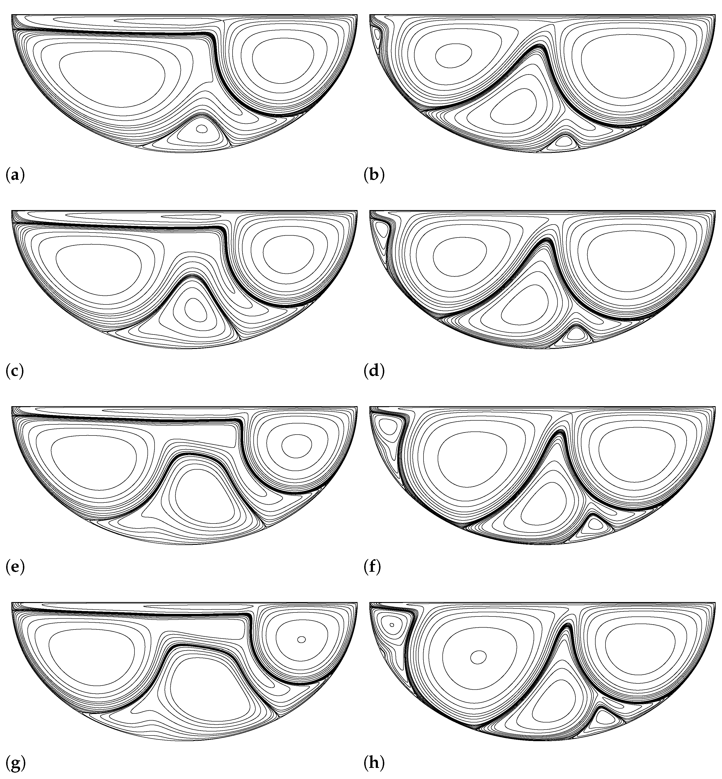
For $D=0.8$ aspect ratio semi-ellipse, we were able to obtain the 2nd solution until $Re=$ 19,000 at maximum, while on the other hand we obtained the 1st solution until $Re=$ 25,000 at maximum. In Figure 15, we give both the 1st and 2nd solutions at various same Reynolds numbers until $Re=$ 19,000. Moreover, Figure 16 shows the evolution of the 1st solution above $Re=$ 19,000 until $Re=$ 25,000.

Similarly, for future references, for the driven semi-elliptical cavity flow with $D=0.8$ aspect ratio, we tabulate the streamfunction ($\psi$) and vorticity ($\omega$) values at the center of the strongest clockwise rotating vortex (i.e., at the location of ${\psi }_{min}$) and also at the center of the strongest counterclockwise rotating vortex (i.e., at the location of ${\psi }_{max}$) together with the x–y locations of these centers for the 1st solution in

Table 7. Minimum and maximum streamfunction values in the 1st solution, corresponding vorticity values and (x,y) locations for $D=0.80$.

	$\mathit{Re}$	$\mathit{\psi }$	$\mathit{\omega }$	x	y
${\psi }_{min}$	1000	−6.3196 $\times {10}^{-2}$	−6.0769	0.1782	−0.1554
	3000	−5.8326 $\times {10}^{-2}$	−6.6326	0.2290	−0.1484
	5000	−5.4667 $\times {10}^{-2}$	−7.0924	0.2567	−0.1414
	7000	−5.1839 $\times {10}^{-2}$	−7.4698	0.2758	−0.1350
	7181	−5.1608 $\times {10}^{-2}$	−7.5018	0.2770	−0.1342
	8000	−5.0580 $\times {10}^{-2}$	−7.6477	0.2827	−0.1321
	10,000	−4.7866 $\times {10}^{-2}$	−8.0869	0.2994	−0.1251
	15,000	−4.3157 $\times {10}^{-2}$	−8.8858	0.3233	−0.1150
	19,000	−4.0239 $\times {10}^{-2}$	−9.4308	0.3391	−0.1082
	20,000	−3.9585 $\times {10}^{-2}$	−9.5596	0.3421	−0.1069
	25,000	−3.6655 $\times {10}^{-2}$	−10.1781	0.3544	−0.1000
${\psi }_{max}$	1000	1.2907 $\times {10}^{-3}$	0.9273	−0.2234	−0.2495
	3000	6.9582 $\times {10}^{-3}$	1.6060	−0.2542	−0.1838
	5000	9.4603 $\times {10}^{-3}$	1.5121	−0.2134	−0.1879
	7000	1.0839 $\times {10}^{-2}$	1.4946	−0.1961	−0.1871
	7181	1.0925 $\times {10}^{-2}$	1.4941	−0.1961	−0.1871
	8000	1.1218 $\times {10}^{-2}$	1.4997	−0.1955	−0.1854
	10,000	1.0803 $\times {10}^{-2}$	1.6823	−0.2409	−0.1696
	15,000	1.1411 $\times {10}^{-2}$	1.8009	−0.2561	−0.1597
	19,000	1.1737 $\times {10}^{-2}$	1.8608	−0.2631	−0.1557
	20,000	1.1780 $\times {10}^{-2}$	1.8736	−0.2645	−0.1548
	25,000	1.1784 $\times {10}^{-2}$	1.9322	−0.2726	−0.1498

and the same for the 2nd solution in

Table 8. Minimum and maximum streamfunction values in the 2nd solution, corresponding vorticity values and (x,y) locations for $D=0.80$.

	$\mathit{Re}$	$\mathit{\psi }$	$\mathit{\omega }$	x	y
${\psi }_{min}$	7182	−6.1157 $\times {10}^{-2}$	−7.1299	0.2374	−0.1479
	8000	−6.0634 $\times {10}^{-2}$	−7.2256	0.2416	−0.1458
	10,000	−5.9233 $\times {10}^{-2}$	−7.4323	0.2506	−0.1430
	15,000	−5.6153 $\times {10}^{-2}$	−7.8163	0.2699	−0.1370
	19,000	−5.4154 $\times {10}^{-2}$	−8.0262	0.2803	−0.1338
${\psi }_{max}$	7182	8.8613 $\times {10}^{-3}$	2.3385	−0.0964	−0.2630
	8000	9.1995 $\times {10}^{-3}$	2.4948	−0.0739	−0.2684
	10,000	9.6247 $\times {10}^{-3}$	2.7295	−0.0429	−0.2778
	15,000	1.0014 $\times {10}^{-2}$	3.1436	0.0109	−0.2857
	19,000	1.0054 $\times {10}^{-2}$	3.3786	0.0393	−0.2889

.

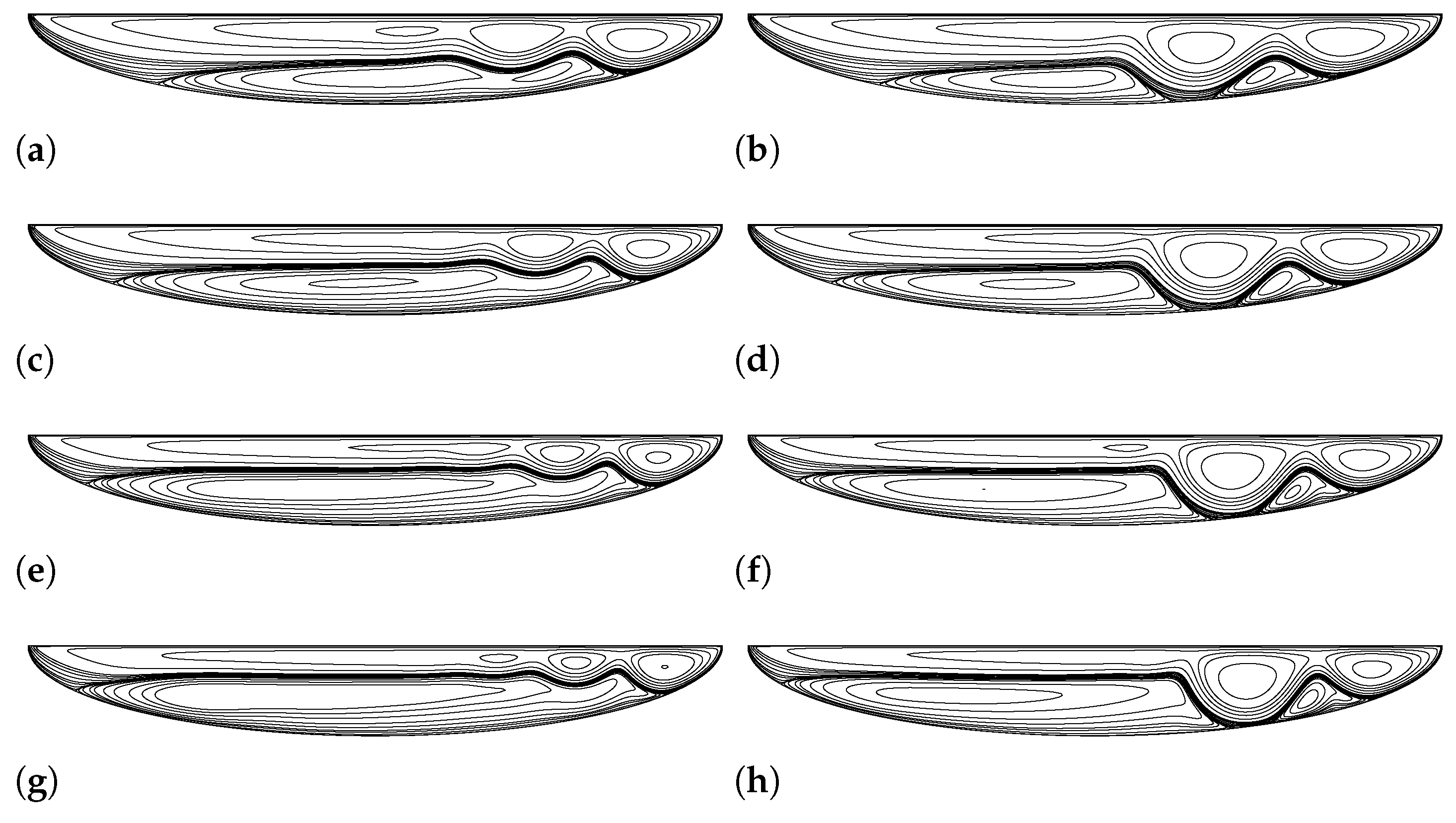
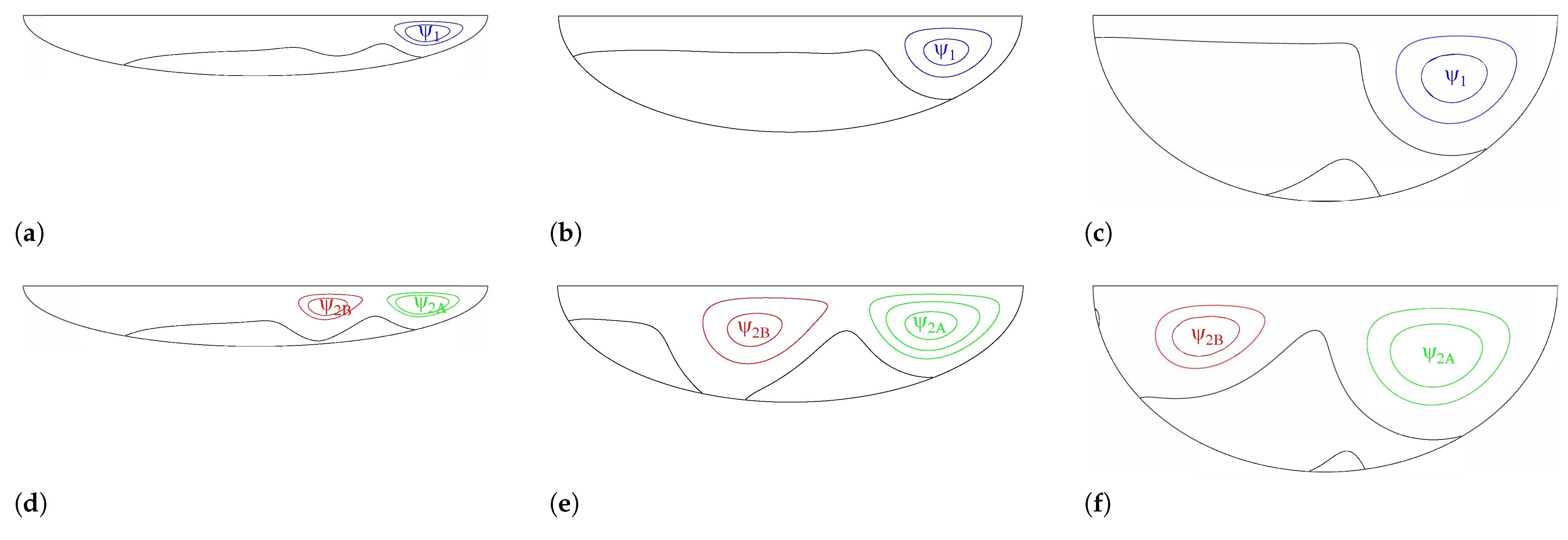
If we look at the solutions given above in Figure 4, Figure 5, Figure 6, Figure 7, Figure 8, Figure 9, Figure 10, Figure 11, Figure 12, Figure 13, Figure 14, Figure 15 and Figure 16, we can notice that the 1st and 2nd solutions of the driven semi-elliptical cavity flow have different characteristics and behavior with respect to the Reynolds number. One of the main differences between the 1st and 2nd solutions is that in the 2nd solution there are two strong local vortex centers in the main clockwise vortex near the top lid; however, there is one in the 1st solution. The schematic views of the vortices in the 1st and 2nd solutions are given in Figure 17. 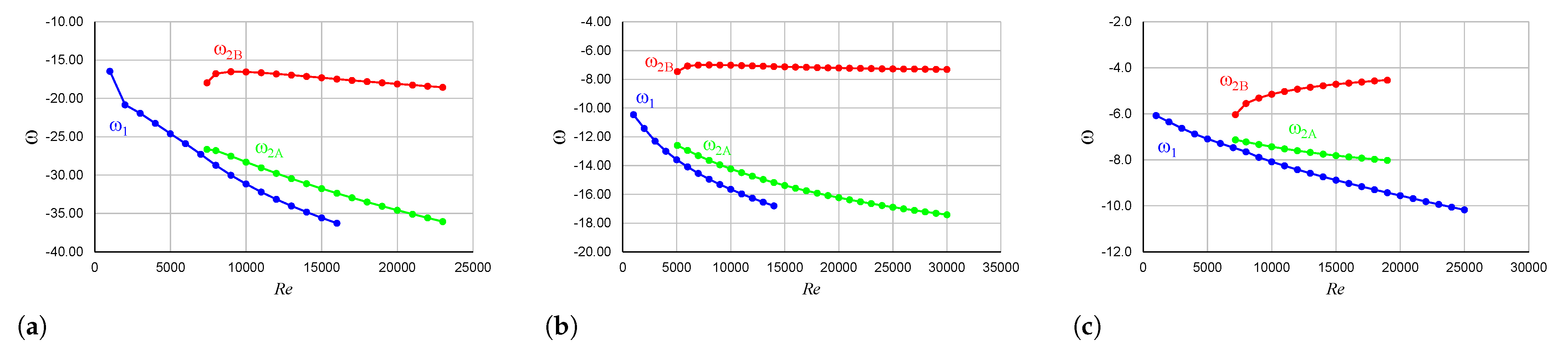In Figure 17, the center of the vortex close to the top moving lid is colored with blue for the 1st solution and the two local centers for the 2nd solution are colored with red and green. In Figure 18, we plot the streamfunction values at the center of these vortex centers (blue, red and green) and also the vorticity values at the same centers in Figure 19 with respect to the Reynolds number.

In Figure 18, in the 1st solution (blue color) in $D=0.26$ aspect ratio, the streamfunction value increases (in absolute value sense) as the Reynolds number increases at small Reynolds numbers and then starts to decrease (in absolute value sense) afterwards. However in $D=0.5$ and $D=0.8$ aspect ratios, the streamfunction value decreases continuously (in absolute value sense) as the Reynolds number increases in the 1st solution (blue color).

On the other hand, in Figure 18, in the 2nd solution (red and green colors), at small Reynolds numbers the streamfunction value at the local center close to the top right corner of the semi-elliptical cavity (green color) is greater than (in absolute value sense) that at the local center close to the center top of the semi-elliptical cavity (red color) for $D=0.26$ aspect ratio. However, as the Reynolds number increases while the streamfunction at the green center decreases (in absolute value sense) that at the red center increases such that red value becomes greater than the green value (in absolute value sense). The same is also true for $D=0.50$ aspect ratio. For $D=0.8$ aspect ratio, even though the trend is the same, the streamfunction at the green center stays greater than (in absolute value sense) that at the red center at all Reynolds numbers.

In Figure 19, in the 1st solution (blue color) the vorticity value at the vortex center increases (in absolute value sense) as the Reynolds number increases for all the aspect ratios considered. The same is also true for the 2nd solution at the green center. In the 2nd solution the vorticity value at the red center first decreases slightly (in absolute value sense) then starts to increase as the Reynolds number increases for $D=0.26$ aspect ratio. In $D=0.50$ aspect ratio, the vorticity value at the red center almost stays constant with respect to the Reynolds number. However, in $D=0.8$ aspect ratio, the vorticity value at the red center continuously decreases (in absolute value sense) as the Reynolds number increases.

As mentioned above, the bifurcation Reynolds number of the driven semi-elliptical cavity flow at which the governing equations start to exhibit multiplicity of solutions changes as the aspect ratio of the semi-ellipse changes. In Figure 20, we plot the variation of the bifurcation Reynolds number for different aspect ratios. Figure 20 shows that starting from the minimum aspect ratio ($D=0.26$), as the aspect ratio increases the bifurcation Reynolds number at first decreases and then starts to increase afterwards while having the minimum bifurcation Reynolds number at $D=0.50$.

4. Conclusions

The semi-elliptical cavity flow is solved numerically for various Reynolds numbers and also for various aspect ratios. The elliptic coordinate system which transforms the geometry conformally and also provides a body fitted coordinate system is used in the formulation. The steady governing flow equations are solved until very low residual levels for numerical accuracy. For the considered driven semi-elliptical cavity flow, the following is concluded:

• The solution of Navier–Stokes equations for incompressible 2D steady flow in a driven semi-elliptical cavity bifurcates at a bifurcation Reynolds number and beyond this bifurcation Reynolds number at least two different solutions exist for the governing equations.
• The solution of Navier–Stokes equations for incompressible 2D steady flow in a driven semi-elliptical cavity bifurcates only for semi ellipses with a vertical-to-horizontal semi-axis ratio (aspect ratio) $0.26\le D\le 0.8$.
• We did not observe bifurcation for semi-ellipses with $D<0.26$ and $0.8>D$ aspect ratios. For these aspect ratio (vertical-to-horizontal semi-axis ratio) semi-ellipses, we find only a single solution for each Reynolds number.
• For semi-ellipses with aspect ratios $0.26\le D\le 0.8$, the bifurcation Reynolds number at which the Navier–Stokes equations start to have multiple solutions at first starts to decrease as D increases; then, after having a minimum around $D=0.5$, the bifurcation Reynolds number starts to increase as D increases further.

Although with the present study at least two different multiplicity solutions of the driven semi-elliptical cavity flow are presented, whether or not the driven semi-elliptical cavity flow has any more multiplicity solutions is an open question for further investigations. Finally detailed streamfunction and vorticity data from the driven semi-elliptical cavity flow are tabulated for future reference.