Abstract
This article studies the estimation of the precision matrix of a high-dimensional Gaussian network. We investigate the graphical selector operator with shrinkage, GSOS for short, to maximize a penalized likelihood function where the elastic net-type penalty is considered as a combination of a norm-one penalty and a targeted Frobenius norm penalty. Numerical illustrations demonstrate that our proposed methodology is a competitive candidate for high-dimensional precision matrix estimation compared to some existing alternatives. We demonstrate the relevance and efficiency of GSOS using a foreign exchange markets dataset and estimate dependency networks for 32 different currencies from 2018 to 2021.
Keywords:
exchange rate; Gaussian graphical model; graphical elastic net; high-penalized log-likelihood; precision matrix estimation; ridge estimation MSC:
62H12; 62J07
1. Introduction
In recent years, covariance and precision matrix estimates have been studied extensively under high-dimensional scenarios. The motivation for these investigations is the argument that traditional likelihood-based techniques perform inaccurately or do not even exist. Examples of these include the graphical lasso algorithm and its extensions ([1,2,3,4,5,6,7]), and the ridge regularization-driven approach for the log-likelihood function ([8,9,10,11]). In addition to considering single (graphical lasso) and Frobenius (graphical ridge) penalties for the precision matrix, some studies have proposed combining both, resulting in an elastic net-type penalty. For instance, the following articles can be mentioned [10,12,13,14].
Despite the vast number of reported studies in the literature on the estimation of precision matrices, there are few reported studies concerning generalization to allow for the incorporation of prior knowledge of a precision matrix. For the Frobenius penalized case we can mentioned [9,10,11]. The only proposals for incorporating target matrices (prior knowledge) for the and elastic net penalty are those of [10,15]. In this paper, we propose the graphical selector operator with shrinkage (GSOS) as a combination of the generalized ridge (ridge with target matrix) and penalty. The main aim of this paper is to present and compare the new precision matrix estimator and propose a novel algorithm for Gaussian graphical models. The numerical study shows that the GSOS estimator is comparable with other available estimators and performs better in most cases than others.
Estimation, Literature Review
In graphical models, Gaussian graphical models are frequently used for modeling conditional dependencies in multivariate data. Dependency structures are determined by estimating the precision matrix through standard methodologies, for instance, a maximum likelihood or the regularized type of maximum likelihood in high-dimensional cases.
Consider random vector ; it follows a multivariate Gaussian distribution with mean vector and positive definite covariance matrix corresponding to conditional independence graph . In terms of mathematics, a pair is a Gaussian graphical model. In these models, the graph and the precision matrix are intimately related. That means that the zeroes in the precision matrix correspond to pairs of conditionally independent features, given all the other variables. In other words, there is no edge between these two variables (nodes) in a graph . Furthermore, two coordinates and are independent if, in the graph , there is no edge between them. Maximum likelihood estimation is a logical technique to estimate the precision matrix for the positive definite matrix ; this estimator is expressed as
where is the sample covariance matrix and the maximum likelihood estimator is equal to . However, two issues might emerge when utilizing this maximum likelihood technique to estimate . First, in the high dimension case , the empirical covariance matrix is singular and hence cannot be inverted to provide an estimate of . Even if p and n are almost equal and is singular, the maximum likelihood estimate for will have a relatively high variance. Second, it is frequently valuable to identify pairs of disconnected variables in a graphical model that are conditionally independent; these correspond to zeroes in . However, in general, (1) will produce an estimate of with no elements equal to zero.
The likelihood function is complemented with a penalty function in high-dimensional settings, which yields the maximum regularized likelihood estimator. Graphical lasso adds an penalty to log-likelihood and induces sparsity of due to maximizing the penalized log-likelihood:
where is a non-negative tuning parameter and denotes the sum of the absolute values of the elements of . This approach was considered almost simultaneously by [1,16,17,18]. Due to the ensuing sparse answer, the graphical lasso estimate has gained significant interest and has become popular; it is still is an active area of research (cf. [6,19,20,21]). In contrast to circumstances where sparsity is advantageous, there are cases when more exact representations of the high-dimensional precision matrix are fundamentally desirable. Furthermore, the genuine (graphical) model does not have to be (very) sparse in terms of having many zero elements. In these situations, we may use a regularization approach that shrinks the estimated precision matrix elements instead of forcing them to be zero. The ridge precision estimator maximizes the log-likelihood augmented by a Frobenius norm, [9] in the most general form presented the ridge estimator as follows
where is the penalty parameter, is a known symmetric and semi-positive definite target matrix, and denotes the Frobenius norm, the sum of the square values of the elements of the matrix . Before estimating, the target matrix is set as an initial guess, toward which the precision estimate is shrunk. Estimator (3) is called the alternative Type I ridge precision estimator, and when the target matrix is equal to zero matrices, the alternative Type II ridge precision estimator. It should be mentioned that [11] considered the estimator mentioned in (3) independently and concurrently, and called it a ridge-type operator for precision matrix estimation (ROPE).
In a recent study in this area, Ref. [10] generalized the ridge inverse covariance estimator to allow for entry-wise penalization. Their proposed estimator shrinks toward a user-specified non-random target matrix and is shown to be positive definite and consistent. Furthermore, they obtained a generalization of the graphical lasso estimator and its elastic net counterpart. Recently, ref. [15] considered elastic net-type penalization (gelnet) for precision matrix estimation in the presence of a diagonal target matrix. They showed that it is possible to adopt the iterative procedure of [10] for the elastic net problem, but it is not computationally attractive.
Under the continuity property of the ridge estimator and apart from sparsity, estimations of the precision matrix with (3) can be far from the actual value . Hence, the motivation of our approach to find a closer estimator. We use the Frobenius norm penalty to penalize the deviation between any primary or initial target estimator and , and tune it to improve the accuracy of the final estimation. Furthermore, the penalty is added to account for sparsity, returning to the well-known elastic net with some added refinement. Therefore, in this paper, we consider combining the estimation approaches (2) and (3) to propose an elastic net-type estimator for the precision matrix: the GSOS.
2. The Proposed Method
Let be the data matrix, including n observations of a dimensional Gaussian distribution with zero mean and positive definite covariance matrix . Consider the following type of estimation problem for estimating the unknown precision matrix based on n observations:
where is a known symmetric and semi-positive definite target matrix. Additionally, , are tuning parameters. Note that if , the precision matrix estimator (4) becomes the ridge estimator that is mentioned in (3).
Using sub-gradient notation and rules from [22], we obtain the following optimal conditions for (4)
where , and the matrix denotes the component-wise signs of with for . The solution of the normal Equation (5) is found by iteratively running over the columns/rows, considering the remaining ones fixed. The update requires that each matrix in (5) is partitioned as follows:
where is a square matrix, is a vector, and is a scalar. and are partitioned similarly. Consider ; using the properties of inverses of block-partitioned matrices, we have that
By substituting and into (7), we have that
Consider and ; then, (9) is equivalent to
where ∗ denotes the element-wise multiplication of two vectors. The conditions mentioned in (10) are KKT optimality conditions for the following box-constrained problem for
By solving the optimization problem (11) and finding the optimum point , can be updated as follows for all
For the diagonal elements of the precision matrix , we consider (5) for diagonal elements
Let ; therefore, we have this quadratic equation
Quadratic Equation (15) has two distinct real roots: positive (acceptable) and negative (unacceptable). Hence, we can update the diagonal elements of the precision matrix with the positive root. Finally, and are updated using normal Equation (5). Our method here is similar to the dpglasso estimator proposed by [5]. Furthermore, we can follow the glasso approach to solve the problem. The fundamental distinction between glasso and dpglasso is that in glasso, is not equal to the inverse of . Furthermore, glasso deals with , whereas dpglasso considers its inverse . Finally, Algorithm 1 shows the procedure for .
| Algorithm 1 GSOS based on dpglasso approach |
|
Glasso Scenario
The following relationship between and is established in glasso
Define ; therefore
Letting , and , then, for every , we have that
Subsequently, the update has the following form
where S is the soft-threshold operator . We cycle through the predictors until convergence. is the optimum point of the following quadratic problem
which corresponds to the normal equations (17). After solving this quadratic problem and finding , we can update . From (5) for the diagonal elements of of the precision matrix, we have that
From (16) we have that ; hence, (21) is equivalent to
Equation (22) has two distinct real roots with positive (acceptable) and negative (unacceptable) signs. Hence, we can update the diagonal elements of the precision matrix with the positive root. Finally, and are updated by (5). Algorithm 2 briefly outlines these steps.
| Algorithm 2 GSOS based on glasso approach |
|
3. Simulation
In this section, the statistical performance of GSOS is compared to some other popular estimators (glasso [1], ROPE or alternative ridge [9,11], and graphical elastic net [15]).
We simulate the data from a multivariate Gaussian distribution , where and are positive definite matrices. Six different models are used to compare the methods (see Appendix A for precision matrices). We evaluate these estimators on the six network structures with nodes and sample size of by implementing Algorithm 2.
- Network 1: A model with compound symmetry structure where and for . In this model, the covariance matrix is structured and non-sparse;
- Network 2. The prototype matrix is used to standardize the precision matrix to possess a unit diagonal. Let , where each off-diagonal entry in is generated independently and equals with probability , or 0 with probability . a is chosen such that the condition number of the matrix is equal to p. Here we have an unstructured and sparse precision matrix;
- Network 3. The precision matrix is defined , where is an matrix with and comes from . The precision matrix of this model is unstructured and non-sparse;
- Network 4. A star model with , and otherwise. This local area network has a structured and sparse precision matrix;
- Network 5. A moving average (MA) model with , and . This covariance matrix is structured and sparse;
- Network 6. A diagonally dominant model. Consider , where is a matrix with zero diagonal elements. Each off-diagonal element of is drawn from a standard uniform distribution. Compute a matrix , where and is the largest row sum of the absolute values of the elements of the matrix . Finally, each off-diagonal element of is chosen as and , where is drawn from uniform distribution with minimum 0 and maximum . This covariance matrix is unstructured and non-sparse.
To calculate the performance measures for all the methods, 100 independent simulations for each network are performed and the average of several loss functions is calculated. The optimal tuning parameter for each method is determined for each simulation run using five-fold cross-validation. For glasso, gelnet, and ROPE, we use the five-fold cross-validation found in the R-package “GLassoElnetFast” with a set value of of 50 elements varying from to 10, and with 20 elements varying from to for gelnet and our estimators. As a target matrix, assume identity matrix and a scalar matrix , where .
3.1. Performance Measures
To calculate the performance of a given estimator , we consider four loss functions that have been used widely in other research in this area (see, e.g., [7,11,14,15]).
Loss Functions
- The Kullback–Leibler loss: ;
- The loss: ;
- The quadratic loss: ;
- The spectral norm loss: , where is the largest eigenvalue of the matrix .
To provide risk measures, the averages of these losses are determined for each method from 100 simulations. Figure 1, Figure 2, Figure 3 and Figure 4 show the final findings. The plot layout is taken from [11]; the columns that go along the little black dots represent loss means. The bars at the top of each column represent standard errors ().
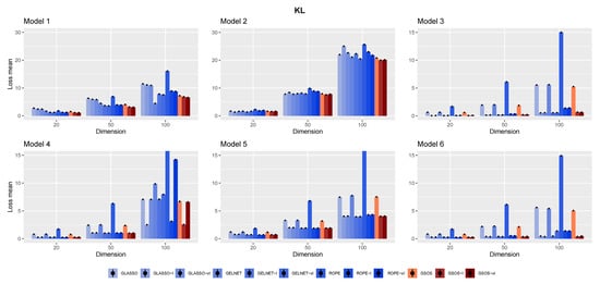
Figure 1.
The mean of Kullback–Leibler loss for the different models and methods based on 100 replications.
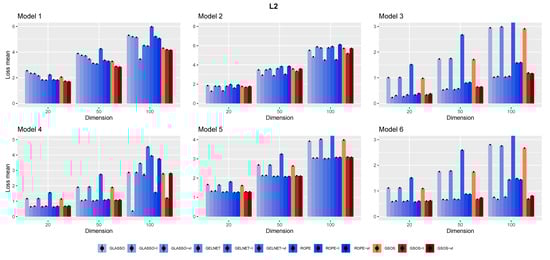
Figure 2.
The mean of loss for the different models and methods based on 100 replications.
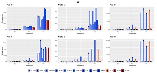
Figure 3.
The mean of quadratic loss for the different models and methods based on 100 replications.
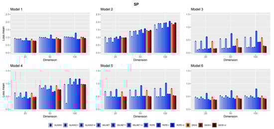
Figure 4.
The mean of spectral norm loss for the different models and methods based on 100 replications.
3.2. Simulation Results
The results for different networks are displayed in Figure 1, Figure 2, Figure 3 and Figure 4. We summarize some observations based on the results as follows:
- In general, as mentioned in [15], it is advantageous to include a target in the methods, since each approach works better with the appropriate target;
- Compared to other alternatives, GSOS is often a considerable contender for high-dimensional precision matrix estimation;
- The question of which target is more effective remains. However, in most cases, our simulations suggest that the identity target matrix works better.
4. Real Data
In the following section, we study market data provided by the Pacific Exchange Rate Service dataset (PERS), which is available on https://fx.sauder.ubc.ca/, accessed on 13 September 2022. PERS provides daily values of the currencies and commodities priced in various base currencies, known as numeraire. We consider 32 different currencies for the four years between 2018 and 2021. The names of these 32 currencies and their abbreviations are listed in Table 1.

Table 1.
List of abbreviations of the considered currencies.
We gather the data initially with the US dollar (USD) as numeraire and then, according to the initial data, calculate all currency exchange rates (for more detail, see [23,24]). After determining all exchange rates, using each of the 32 currencies as a numeraire, we compute the daily log returns of the remaining 31 currencies. We estimate the related covariance and precision matrices based on all possible exchange currencies (496 different exchanges). We apply our proposed estimator GSOS, with the scalar matrix as a target for four-year and annual data separately (the five-fold cross-validation is considered in selecting the tuning parameters). The estimated networks are presented in Figure 5, Figure 6, Figure 7, Figure 8 and Figure 9; it should be mentioned that we consider 50 of the strongest partial correlations.
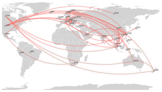
Figure 5.
Estimated currency network based on 2018 to 2021 foreign exchange markets data.
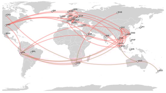
Figure 6.
Estimated currency network based on 2018 foreign exchange markets data.
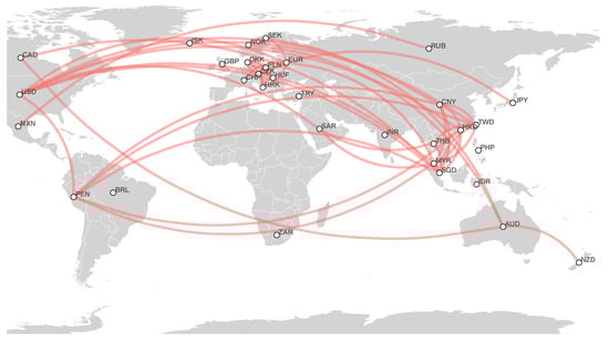
Figure 7.
Estimated currency network based on 2019 foreign exchange markets data.
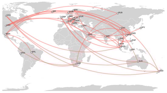
Figure 8.
Estimated currency network based on 2020 foreign exchange markets data.
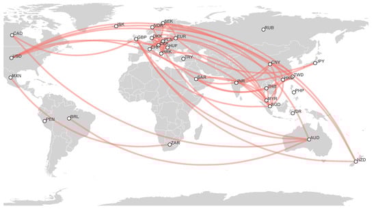
Figure 9.
Estimated currency network based on 2021 foreign exchange markets data.
Real Data Results
To report the analytical results, we consider the different thresholds for partial correlation to explain the most important relations between considered currencies. We apply filtering by considering only ones that exceed those thresholds to explain how these networks are formed.
- 2018–2021 network: First, strong partial correlations appear between European currencies: DKK, HRK, CZK, PLN, HUF, CHF, and EUR. Additionally, we find a cluster that consists of HKD, SAR, CNY, TWD, SGD, and USD. Considering a smaller threshold, one notices the partial correlation between the Oceania couple of AUD and NZD and CAD, and the joining of EUR to the USD-based cluster, which connects European currencies to this cluster. Finally, a rather interesting cluster centered around a Latin American currency, MXN, appears, which consists of BRL, ZAR, and RUB;
- 2018 network: We observe strong correlations between European currencies: DKK, HRK, CZK, PLN, HUF, and EUR. The USD-based cluster here consists of HKD, PEN, TWD, SGD, CNY, THB, and MYR. The EUR currency connects these two major clusters. We find the relation between the Oceania couple AUD and NZD and CAD for a smaller threshold. In addition, a cluster between the Latin American, African, and Asian currencies MXN, ZAR, and RUB is noteworthy;
- 2019 network: Similar to the 2018 network, we have strong and connected European currencies: DKK, HRK, CZK, PLN, and HUF. The USD-based cluster is formed by HKD, SAR, TWD, SGD, CNY, and MYR at first; by considering a smaller threshold, we find other currencies such as PEN and THB. We observe that EUR connects these two clusters, and another cluster consists of AUD, NZD, NOK, and SEK;
- 2020 network: This year, we observe the USD cluster as follows: HKD, SAR, TWD, SGD, and CNY. We can see MYR, PHP, and THB as a disjointed clique (every two distinct vertices are adjacent). Regarding European currencies, EUR and CHF have a connecting role between this cluster and the USD-based cluster. The European currency cluster consists of DKK, HRK, CZK, PLN, and HUF. In addition, we observe two other clusters: the Oceania couple AUD and NZD with CAD and GBP, and MXN, BRL, ZAR, and RUB. These two clusters have a connection to European currencies by SEK;
- 2021 network: As previously, we observe that the USD-based cluster consists of HKD, SAR, TWD, CNY, and SGD. DKK, HRK, CZK, HUF, PLN, CHF, SEK, and EUR form a European currency cluster, which is connected to the USD cluster by EUR. In addition, we discover an interesting cluster centered around AUD consisting of NZD, CAD, NOK, and GBP. Considering a smaller threshold, we find more relations in the last cluster and considerable partial correlations between AUD, NZD, NOK, and SEK. This year, we see a strong partial correlation between GBP and SGD, which has never been observed before. Finally, we have a small cluster consisting of three Latin American, Asian, and African currencies: MXN, RUB, and ZAR.
5. Discussion
This section provides a summary of the paper and highlights the results. Additionally, we address some limitations of the research and gaps for future research. Finally, we review the findings and the results of the proposed method: GSOS.
5.1. Summary
In this paper, we proposed two methods to estimate a precision matrix in multivariate Gaussian settings. Estimating a precision matrix is one of the most critical tools for reconstructing an undirected graphical model expressing conditional dependencies between variables. Furthermore, obtaining an estimated network of partial correlations with a suitable rescaling of the precision matrix is possible.
We focused on the high-dimensional case to obtain regularized and sparse estimates considering the elastic net-type penalty. This penalty is a combination of the Frobenius norm when a target matrix is taken into account and the norm penalty to create sparsity. The first method, Algorithm 1, employs the dpglasso technique proposed by [5] to find penalized log-likelihood estimation. The second method, Algorithm 2, follows a similar approach to glasso, as studied by [1], and solves optimization problems by turning them into quadratic problems.
We conducted a simulation study to test the proposed algorithms using three different sample sizes and six common network structures reflecting various forms of conditional dependence. To calculate the performance measures for all the methods, we considered 100 independent simulations for each network; we presented the average of the Kullback–Leibler, , quadratic, and spectral norm loss functions. The optimal tuning parameters for each method were determined using five-fold cross-validation for each simulation run.
Lastly, we presented an empirical study of the network between 32 currencies for the years between 2018 and 2021. We estimated annual and four-year networks according to these years. We evaluated the high-dimensional precision matrix in every yearly network in this real data study.
5.2. Contributions
We added sparsity to the alternative ridge estimator by considering the norm as an additional penalty. In this area, [15] also focused on the elastic net-type penalties for a Gaussian log-likelihood-based precision matrix estimation called gelnet. However, they simultaneously considered the target matrix for the and Frobenius norm. Therefore, we cannot obtain our estimator from gelnet when considering nonzero target matrices. These relations encouraged us to choose glasso, alternative ridge, and gelnet as competitor estimators to compare with our proposed estimator, GSOS.
We used the R programming language [25] and the “GLassoElnetFast” package for the simulation study; the codes are available on https://github.com/Azamkheyri/GSOS.git, accessed on 27 October 2022. In terms of simulation results, GSOS outperformed alternative ridge with most of the underlying structures in the high-dimensional case for all considered sample sizes. GSOS and gelnet, in most cases, behaved almost similarly, but in Network 4 for the Kullback–Leibler and risk measures, GSOS significantly outperformed gelnet.
On glasso: according to the Kullback–Leibler risk measure, GSOS and glasso performed similarly, except in Networks 1 and 2, where GSOS performed better. For the measure, GSOS performed better in Network 1, while for the quadratic risk measure, their behaviors are different; in three networks, GSOS outperformed glasso and for the remainder, glasso was better. Therefore, our proposed estimator is an efficient way to estimate precision matrices for the high-dimension Gaussian graphical models.
Finally, we added a real data example, the PERS dataset, and estimated four annual and one four-year dependency networks from 2018 to 2021. Since the log returns must be calculated using data from two consecutive days, we removed from our research those currencies for which there were at least ten missing values for exchange rates with the USD. Therefore, we estimated high-dimension precision matrices with GSOS for 32 currencies worldwide.
5.3. Strengths and Limitations
As we mentioned before, we considered the elastic net-type penalty for the Gaussian log-likelihood problem to estimate the precision matrix. The most important strength of our proposal is that this kind of penalty could help simultaneously obtain the advantages of the Frobenius norm and -penalized estimations. We could not prove that our proposed estimator mathematically outperforms the known methods; this might be considered as a limitation. However, we illustrated the performance of the GSOS estimator with a simulation study under six different frequently used dependency networks in the literature.
Our simulation results are related to the considered network’s structure and performance measures; hence, they are not general. Furthermore, despite our proposed estimator’s considerable statistical performance, there is no overall winner.
Finally, because of the presence of missing data in the foreign exchange markets and the fact that log returns of the data have to be calculated from two consecutive days, only those currencies in which there were less than ten missing values for exchange rates based on USD were considered.
5.4. Future Work
For future research, we will consider studying the asymptotic behavior of our suggested estimators. In addition, while all the recommended estimators depend on the multivariate Gaussian assumption, we might also consider ways to do away with it by proposing distribution-free approaches or looking at other distributions to capture the data’s properties better. The relationship between the values of two tuning parameters— and —might be worthwhile to investigate.
Moreover, the considered real data example has more potential for further study, for instance, considering long-term studies and interpreting the results based on geographic, economic, or political factors.
6. Conclusions
The proposed precision estimator is based on the penalty for sparsity on Gaussian log-likelihood and penalization with Frobenius norm shrinkage to an arbitrary non-random target value. We proposed two algorithms based on gradient descent (glasso) and the box-constrained quadratic program (dpglasso). Our approach is similar to gelnet by [15], but with some refinement; the estimator proposed here cannot be obtained from gelnet. Compared to other alternatives, the simulation study illustrated that our proposed strategy is a good competitor for high-dimensional precision matrix estimation. Additionally, we presented an empirical analysis of a network of 32 popular currencies and estimated yearly and four-year dependency networks.
Author Contributions
Funding acquisition, A.B. and M.A.; methodology, A.K., A.B. and M.A.; project administration, A.B.; supervision, A.B. and M.A.; validation, A.K., A.B. and M.A.; writing—original draft, A.K.; writing—review and editing, A.B. and M.A. All authors have read and agreed to the published version of the manuscript.
Funding
This work was based upon research supported in part by the National Research Foundation (NRF) of South Africa, Ref.: SRUG190308422768, grant no. 120839; the South African DST-NRF-MRC SARChI Research Chair in Biostatistics (grant no. 114613); and STATOMET at the Department of Statistics at the University of Pretoria. The third author’s research (M. Arashi) is supported by a grant from Ferdowsi University of Mashhad (N.2/58091).
Data Availability Statement
The data under consideration in this study is in the public domain.
Acknowledgments
We would like to sincerely thank the two anonymous reviewers for their constructive comments, which led us to add many details to the paper and improve the presentation.
Conflicts of Interest
The funders had no role in the design of the study; in the collection, analyses, or interpretation of data; in the writing of the manuscript, or in the decision to publish the results.
Abbreviations
The following abbreviations are used in this manuscript:
| GLASSO | Graphical lasso with zero target matrix |
| GLASSO-I | Graphical lasso with identity target matrix |
| GLASSO-vI | Graphical lasso with scalar target matrix |
| GELNET | Graphical elastic net with zero target matrix |
| GELNET-I | Graphical elastic net with identity target matrix |
| GELNET-vI | Graphical elastic net with scalar target matrix |
| ROPE | ROPE with zero target matrix |
| ROPE-I | ROPE with identity target matrix |
| ROPE-vI | ROPE with scalar target matrix |
| GSOS | GSOS with zero target matrix |
| GSOS-I | GSOS with identity target matrix |
| GSOS-vI | GSOS with scalar target matrix |
Appendix A
Figure A1 shows the precision matrices of the considered networks in the simulation study.

Figure A1.
Precision matrices (diagonal elements ignored).
Figure A1.
Precision matrices (diagonal elements ignored).

References
- Friedman, J.; Hastie, T.; Tibshirani, R. Sparse inverse covariance estimation with the graphical lasso. Biostatistics 2008, 9, 432–441. [Google Scholar] [CrossRef] [PubMed]
- Fan, J.; Feng, Y.; Wu, Y. Network exploration via the adaptive LASSO and SCAD penalties. Ann. Appl. Stat. 2009, 3, 521. [Google Scholar] [CrossRef] [PubMed]
- Bien, J.; Tibshirani, R.J. Sparse estimation of a covariance matrix. Biometrika 2011, 98, 807–820. [Google Scholar] [CrossRef] [PubMed]
- Witten, D.M.; Friedman, J.H.; Simon, N. New insights and faster computations for the graphical lasso. J. Comput. Gr. Stat. 2011, 20, 892–900. [Google Scholar] [CrossRef]
- Mazumder, R.; Hastie, T. The graphical lasso: New insights and alternatives. Electron. J. Stat. 2012, 6, 2125. [Google Scholar] [CrossRef]
- Danaher, P.; Wang, P.; Witten, D.M. The joint graphical lasso for inverse covariance estimation across multiple classes. J. R. Stat. Soc. Ser. B (Statist. Methodol.) 2014, 76, 373–397. [Google Scholar] [CrossRef]
- Avagyan, V.; Alonso, A.M.; Nogales, F.J. Improving the graphical lasso estimation for the precision matrix through roots of the sample covariance matrix. J. Comput. Graph. Stat. 2017, 26, 865–872. [Google Scholar] [CrossRef]
- Warton, D.I. Penalized normal likelihood and ridge regularization of correlation and covariance matrices. J. Am. Stat. Assoc. 2008, 103, 340–349. [Google Scholar] [CrossRef]
- Van Wieringen, W.N.; Peeters, C.F. Ridge estimation of inverse covariance matrices from high-dimensional data. Comput. Stat. Data Anal. 2016, 103, 284–303. [Google Scholar] [CrossRef]
- van Wieringen, W.N. The generalized ridge estimator of the inverse covariance matrix. J. Comput. Graph. Stat. 2019, 28, 932–942. [Google Scholar] [CrossRef]
- Kuismin, M.; Kemppainen, J.; Sillanpää, M. Precision matrix estimation with ROPE. J. Comput. Graph. Stat. 2017, 26, 682–694. [Google Scholar] [CrossRef][Green Version]
- Rothman, A.J. Positive definite estimators of large covariance matrices. Biometrika 2012, 99, 733–740. [Google Scholar] [CrossRef]
- Atchadé, Y.F.; Mazumder, R.; Chen, J. Scalable computation of regularized precision matrices via stochastic optimization. arXiv 2015, arXiv:1509.00426. [Google Scholar]
- Bernardini, D.; Paterlini, S.; Taufer, E. New estimation approaches for graphical models with elastic net penalty. arXiv 2021, arXiv:2102.01053. [Google Scholar] [CrossRef]
- Kovács, S.; Ruckstuhl, T.; Obrist, H.; Bühlmann, P. Graphical Elastic Net and Target Matrices: Fast Algorithms and Software for Sparse Precision Matrix Estimation. arXiv 2021, arXiv:2101.02148. [Google Scholar]
- Yuan, M.; Lin, Y. Model selection and estimation in the Gaussian graphical model. Biometrika 2007, 94, 19–35. [Google Scholar] [CrossRef]
- Banerjee, O.; El Ghaoui, L.; d’Aspremont, A. Model selection through sparse maximum likelihood estimation for multivariate Gaussian or binary data. J. Mach. Learn. Res. 2008, 9, 485–516. [Google Scholar]
- Yuan, M. Efficient computation of ℓ1 regularized estimates in Gaussian graphical models. J. Comput. Graph. Stat. 2008, 17, 809–826. [Google Scholar] [CrossRef]
- Guo, J.; Levina, E.; Michailidis, G.; Zhu, J. Joint estimation of multiple graphical models. Biometrika 2011, 98, 1–15. [Google Scholar] [CrossRef]
- Shan, L.; Kim, I. Joint estimation of multiple Gaussian graphical models across unbalanced classes. Comput. Stat. Data Anal. 2018, 121, 89–103. [Google Scholar] [CrossRef]
- Londschien, M.; Kovács, S.; Bühlmann, P. Change-point detection for graphical models in the presence of missing values. J. Comput. Graph. Stat. 2021, 30, 768–779. [Google Scholar] [CrossRef]
- Boyd, S.; Boyd, S.P.; Vandenberghe, L. Convex Optimization; Cambridge University Press: Cambridge, UK, 2004. [Google Scholar]
- Basnarkov, L.; Stojkoski, V.; Utkovski, Z.; Kocarev, L. Correlation patterns in foreign exchange markets. Phys. A Stat. Mech. Its Appl. 2019, 525, 1026–1037. [Google Scholar] [CrossRef]
- Fenn, D.J.; Porter, M.A.; Mucha, P.J.; McDonald, M.; Williams, S.; Johnson, N.F.; Jones, N.S. Dynamical clustering of exchange rates. Quant. Financ. 2012, 12, 1493–1520. [Google Scholar] [CrossRef]
- R Core Team. R: A Language and Environment for Statistical Computing; R Foundation for Statistical Computing: Vienna, Austria, 2022. [Google Scholar]


Publisher’s Note: MDPI stays neutral with regard to jurisdictional claims in published maps and institutional affiliations. |
© 2022 by the authors. Licensee MDPI, Basel, Switzerland. This article is an open access article distributed under the terms and conditions of the Creative Commons Attribution (CC BY) license (https://creativecommons.org/licenses/by/4.0/).