Article

An Enhanced U-Net Approach for Segmentation of Aeroengine Hollow Turbine Blade

1
School of Advanced Manufacturing Engineering, Chongqing University of Posts and Telecommunications, Chongqing 400065, China
2
State Key Laboratory of Mechanical Transmission, Chongqing University, Chongqing 400044, China
*
Author to whom correspondence should be addressed.
Mathematics 2022, 10(22), 4230; https://doi.org/10.3390/math10224230
Submission received: 10 October 2022 / Revised: 9 November 2022 / Accepted: 11 November 2022 / Published: 12 November 2022
(This article belongs to the Section Mathematics and Computer Science)

Abstract

:
The hollow turbine blade plays an important role in the propulsion of the aeroengine. However, due to its complex hollow structure and nickel-based superalloys material property, only industrial computed tomography (ICT) could realize its nondestructive detection with sufficient intuitiveness. The ICT detection precision mainly depends on the segmentation accuracy of target ICT images. However, because the hollow turbine blade is made of special superalloys and contains many small unique structures such as film cooling holes, exhaust edges, etc., the ICT image quality of the hollow turbine blades is often deficient, with artifacts, low contrast, and inhomogeneity scattered around the blade contour, making it hard for traditional mathematical model-based methods to acquire satisfying segmentation precision. Therefore, this paper presents a deep learning-based approach, i.e., the enhanced U-net with multiscale inputs, dense blocks, focal loss function, and residual path in the skip connection to realize the high-precision segmentation of the hollow turbine blade. The experimental results show that our proposed enhanced U-net can achieve better segmentation accuracy for practical turbine blades than conventional U-net and traditional mathematical model-based methods.

1. Introduction

As an important part of the aeroengine, the hollow turbine blade is made of special nickel-based superalloys and has a complex internal multicavity structure with closed curved surfaces to adapt to the high temperature and pressure working conditions. Its thin-walled structure makes it hard for traditional detection methods, such as three-coordinate measurement, ultrasound, etc., to detect it qualitatively and quantitatively [1]. Computed tomography (CT) is a prospective nondestructive detection method that can “see through” the test object. Hence, CT detection has been widely applied in tasks where traditional methods cannot perform accurate detections, such as material science [2], industrial applications [3], medical imaging [4], geosciences [5], civil engineering [6], etc.
However, due to the hollow turbine blade’s complex structure and special material properties, the industrial computed tomography (ICT) images contain blurred and low-contrast small structures whose precise contours are hard to extract [7], which greatly affects their ICT detection accuracy, as shown in Figure 1. Typically, there are two ways to solve this problem: (1) improve the ICT image quality and (2) increase the precision of image segmentation methods. The first approach requires better hardware of X-ray source, flat panel detector, etc., which is expensive and laborious. Therefore, many efforts have been made to increase the segmentation accuracy of the turbine blade.
Typical ICT segmentation methods are derived from natural image processing methods, i.e., they are modified to adapt to ICT image characteristics. Popular ICT image segmentation methods include thresholding method [8], morphological method [9], edge detection [2], active contours [10], fuzzy methods [11], etc. Among them, thresholding is simple and fast. However, thresholding cannot deal with images with artifacts and noise well [12]. Morphological methods can deal with noisy images but are easily affected by artifacts [13]. Edge detection methods are fast but can only handle images without noise, inhomogeneity, and artifacts [14]. Active contours can handle noise and inhomogeneity well but is time-consuming [15]. Fuzzy methods are sensitive to noise and low contrast [16].
With the development of computer technology, deep neural networks have made great progress in the fields of machine learning and computer vision [17]. Using a deep neural network to segment an object among the background is to train the network for specific image segmentation tasks, where the network architecture and the training methods will all affect the final segmentation accuracy [18]. Common deep learning architectures include convolutional neural networks (CNNs), recurrent neural networks (RNNs), encoder–decoder models, and generative adversarial networks (GANs) [19]. Image segmentation models are basically derived from these network architectures with the help of encoders, decoders, skip-connections and dilation modifications, etc. Typical image segmentation methods are fully convolutional networks (FCNs) [20], encoder–decoder approaches [21], multiscale and pyramid network-based models [22], R-CNN approaches [23], dilated convolutional networks [24], RNN-based approaches [25], and attention- [26] and GAN [27]-based models. Among different network structures, the U-net approach is an efficient segmentation network that is very suitable for images with microscopic details, such as medical images with blood vessels and ICT images with complex microstructures [28]. Compared with conventional encoder–decoder convolution neural networks, the bypass connections in the U-net could compensate for the lost high-frequency details during pooling [29].
The most widely applied area of the U-net is medical image segmentation [30]. For example, Baltruschat et al. used the U-net to segment the bone implant, which achieved the overall best mean IoU = 0.906 [31]. Ghosh et al. combined the U-net with the VGG-16 network to segment brain tumors and achieved a pixel accuracy of 0.9975 [32]. Guo et al. used the U-net for breast ultrasound image segmentation and realized the average IOU of 82.7% (±0.02), while Khaled et al. obtained a mean dice similarity coefficient (DSC) of 0.680 (0.802 for main lesions) for dynamic contrast enhanced magnetic resonance imaging (DCE-MRI) with the help of the U-net [33]. Li et al. also applied the U-net in isotropic quantitative differential phase contrast imaging, the result of which shows that the quantitative phase value in the ROI is recovered from 66% to 97% compared with the ground truth [34]. Lee et al. proposed the FUS-net based on the U-net for interference filtering in high-intensity-focused ultrasound images, which performs 15% better than stacked autoencoders (SAE) on evaluated test datasets [35]. Moreover, Rocha et al. compared the U-net with the conventional sliding band filter (SBF) approach, the experimental results of which indicate that the U-net-based models yield more identical results to the ground truth [36].
Because the conventional U-net will pass the low-resolution content through the skip-connections, the high-resolution edge information of the input image may not be sufficiently extracted, resulting in a reduced segmentation accuracy of tiny objects. Many efforts have been made to improve the performance of the conventional U-net. For example, Han et al. proposed a dual-frame U-net by adding a residual path after the pooling and before the unpooling operations for sparse-view CT reconstruction, which received a better peak-signal-to-noise ratio (PSNR) performance at the condition of x2 down-sampling factor compared with conventional U-net [29]. Seo et al. added a residual path with deconvolution and activation operations to the skip connection of the U-net to avoid duplication of low-resolution information of features, which realized a DSC of 98.51% and 89.72 % for liver and liver–tumor segmentation [37], respectively. In addition, Man et al. applied the deformable convolution in the conventional U-net for pancreas segmentation, which can capture the geometry-aware information of the head and tail end of the pancreas with a mean DSC of 86.93 ± 4.92% [38]. Hiasa et al. modified the U-net by inserting the dropout layer before each max pooling layer and after each up-convolution layer, which realized a dice coefficient (DC) of 0.891 ± 0.016 and an average symmetric surface distance (ASD) of 0.994 ± 0.230 mm for muscle segmentation [39]. Moreover, He et al. proposed a hierarchically fused U-net by incorporating contour awareness for prostate segmentation, which achieved an overall DSC accuracy of 0.878 ± 0.029 [40].
In addition to medical imaging, the U-net is also suitable for industrial applications. For example, Wang et al. used the U-net to remove artifacts produced by the projection of the static parts in CT reconstruction, which realized the recovery of rotating part details during in situ nondestructive testing of airplane engines [41]. Li et al. realized acoustic interference striation (AIS) recovery using the U-net. The test results in range-dependent waveguides with nonlinear internal waves demonstrated its effectiveness under different signal-to-noise ratios and different amplitudes and widths [42]. Xiao et al. realized precise ore mask segmentation (IOU = 92.07%) via U-net with the combination of the boundary mask fusion block [43].
In summary, the U-net architecture has good segmentation performance for grayscale images compared to conventional single-resolution neural networks. However, the ICT images of the hollow turbine blade contain severe inhomogeneity and cone beam artifacts [7], which are not conducive to accurate U-net segmentation of the turbine blade edge. At the same time, the turbine blades contain microstructures such as film cooling holes and exhaust edges that are not easy to detect via the U-net. Therefore, this paper presents an enhanced U-net with multiscale input and structural modifications to improve the segmentation performance of the conventional U-net. The contribution of this paper is that a deep-learning approach for the segmentation of the hollow turbine blade is proposed, which is a relatively novel approach in the area of aeroengine engineering. Sample expansion and modification to the U-net are conducted to improve the network’s processing effect on inhomogeneity, noise, and artifacts, providing a feasible solution for similar industrial nondestructive testing problems.
The rest of this paper is arranged as follows. Section 2 introduces our enhanced U-net; Section 3 testifies our proposed method by experiments; Section 4 concludes our paper.

2. Materials and Methods

2.1. Preprocessing of Training Data

2.1.1. Data Source

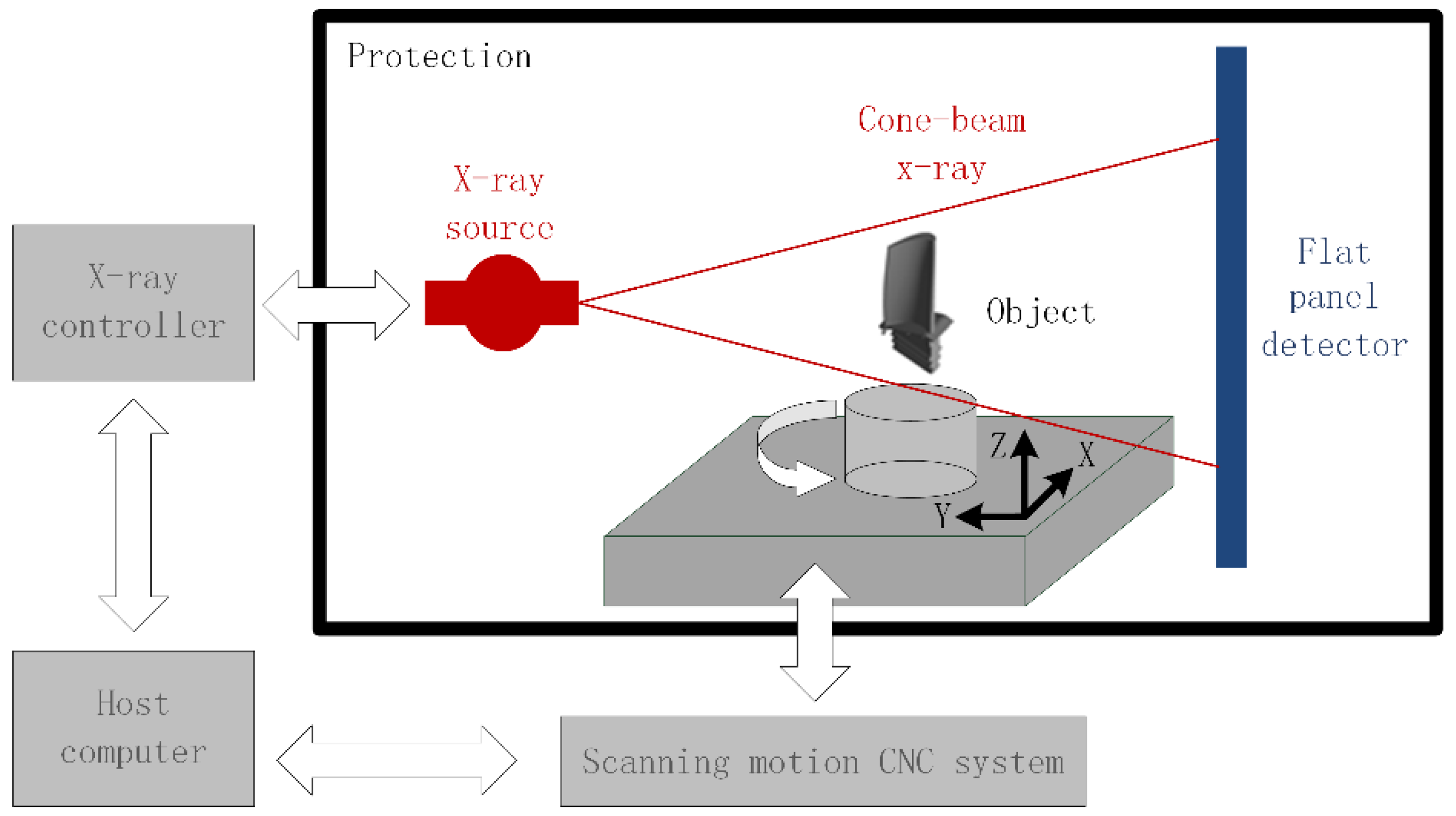
The schematic diagram of the ICT scanning system is shown in Figure 2. The workpiece to be detected is placed on the rotary table controlled by the computer numerical control (CNC) system. Then the X-ray source projects an X-ray to penetrate the workpiece and leaves a projection on the flat panel detector. By rotating the workpiece at 360 degrees, the projection data of the workpiece in all directions can be obtained. After that, the ICT reconstruction algorithm is used to obtain the CT slice images of the workpiece.
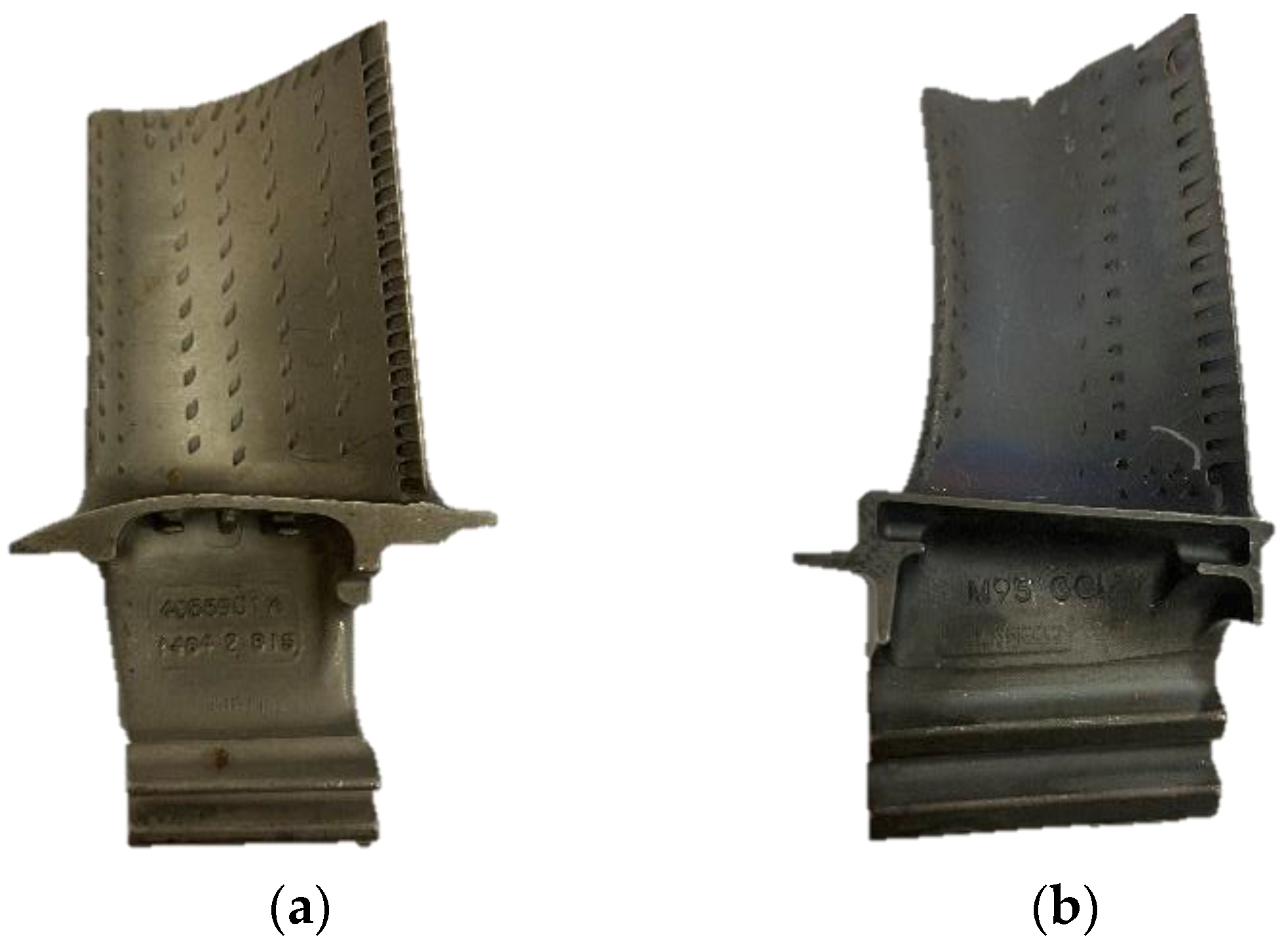
The segmentation objects of this paper are the high-pressure turbine blades of the CFM56-7BE and the Pratt & Whitney F100 aeroengine, as shown in Figure 3. The ICT scanning parameters are as follows: equipment model: AX-4000CT; radiation source: FineTec microfocus radiation source; detector: VAREX XRD4343N (formerly PE); scanning parameters: 400 kV voltage and 1.5 mA current.

2.1.2. Data Augmentation

To augment the training data for segmentation of input images, this paper adopted the following augmentation approaches:
  • Translation Transformation
The translation transformation of an image generally moves the image as a whole along the X direction or the Y direction or both the X and Y directions at the same time. After the translation, blank pixels will be generated, which could be handled via filling with black, assuming that the entire image moves Δ x along the X direction and Δ y along the Y direction. Then the transformation matrix from the original pixel ( x 0 , y 0 ) to the transformed point ( x , y ) can be expressed as Equation (1):
[ x y 1 ] = [ 1 0 Δ x 0 1 Δ y 0 0 1 ] [ x 0 y 0 1 ]
  • Mirror Transformation
Mirror transformation includes horizontal mirroring and vertical mirroring. The image size remains unchanged before and after the mirror transformation, and no new blank pixels are generated. Suppose the image height is h , and the width is w . Then the transformation matrix from the original pixel ( x 0 , y 0 ) to the transformed point ( x , y ) via horizontal mirroring and vertical mirroring can be expressed in Equations (2) and (3):
[ x y 1 ] = [ 1 0 w 0 1 0 0 0 1 ] [ x 0 y 0 1 ]
[ x y 1 ] = [ 1 0 0 0 1 h 0 0 1 ] [ x 0 y 0 1 ]
  • Rotation Transformation
Rotation transformation typically rotates the image around its center. Rotate the original image by θ clockwise around the center. Then the transformation matrix from the original pixel ( x 0 , y 0 ) to the transformed point ( x , y ) via rotation transformation can be expressed as Equation (4):
[ x y 1 ] = [ cos θ sin θ 0 sin θ cos θ 0 0 0 1 ] [ x 0 y 0 1 ]
  • Scaling Transformation
The scaling transformation in data augmentation is helpful for neural networks to learn features of different scales, which need to be cropped or filled with blank pixels (this paper filled the blank pixel with zero) to remain the same size as the original image when the scale ratio is above or below one.

2.2. Architecture of the Enhanced U-net

The traditional U-net is an end-to-end encoder–decoder-based image semantic segmentation network, which is mainly composed of the encoder, the decoder, and the jump connection. The architecture of the U-net resembles a capital “U” letter, which is a symmetrical network with an encoder on the left and the decoder on the right. The encoder is mainly used to extract the image’s features, location, semantics, and other information, which is composed of several groups of “convolution + batchnormalization + Relu” operations followed by “Maxpooling” to realize the nonlinear expression capability of the network. Unlike the encoder, the decoder is used for up-sampling, restoring, and decoding the learned abstract semantic features via up-convolution operations to recover the image’s semantic information gradually. The input of each decoder layer is fused with the features of the corresponding ender layer through a jump connection to obtain enough image features at different scales. A 1*1 convolution operation will connect the output of the decoder and Softmax operation to map feature maps learned by the U-net network to the number of categories that need to be divided. Then each pixel in the original image is classified according to the probability value generated by the U-net network. Compared with conventional fully convolutional networks, the U-net network performs well in dealing with image contour segmentation due to the deep multiscale fusion of high-level and low-level features through skip connection operations.
In the U-net, the deep feature maps near the end of the network can learn strong abstract semantic information. In contrast, the feature maps near the input layer can learn detailed information about the input, including target location, edge, and other features. Therefore, the noise, low contrast, and inhomogeneity of the input images will jeopardize the details of U-net feather maps and significantly affect the accuracy of the overall segmentation performance. To solve this dilemma, this paper proposed an enhanced U-net for the segmentation of the aeroengine hollow turbine blade. The following improvements are applied to the original U-net network.
(1) Multiscale input: To provide the network with enough image information from different scales, this paper adopted the multiscale input for the network. The advantage of this operation is that the average pooling down-sampling of the original image will not increase the computation complexity of the parameters in the network while the network width of the decoder path is extended.
(2) Dense block: Different from the common hierarchical convolutional neural network block, the dense block makes full use of the feature information at each level of the block, while the hierarchical network block only uses the feature map from the previous layer or two layers without considering the lower level. For each layer, the features of all previous layers in this block are used as input. Its own feature map is used as input for all subsequent layers, which can alleviate the gradient disappearance problem at a certain level and strengthen the full utilization of each feature map.
Let x0, x1, …, xl−1 represent the output of the front l−1 layers in the current neural network block, and xl represent the output of the lth convolutional layer; then the dense block can be expressed as follows:
x l = H l ( [ x 0 , x 1 , , x l 1 ] )
where Hl(*) represents a certain nonlinear composite function of the lth convolutional layer.
(3) Focal loss function: For the segmentation task of turbine blades, the proportion of blades in the input image is relatively small, i.e., the background is much larger than the area occupied by the object, which causes a serious imbalance between positive and negative samples. During neural network training, the model is more inclined to learn background features, and it is easy to judge positive samples that are difficult to learn as negative samples. To solve this imbalance issue, this paper used the Focal loss function to pay more attention to the contour pixels:
L = [ α ( 1 y ^ ) γ y log y ^ + ( 1 α ) y ^ γ ( 1 y ) log ( 1 y ^ ) ]
In Equation (6), y and y ^ represent the network’s true value and prediction value; α is the weighting factor, which is used to balance the imbalance of positive and negative samples; γ represents the modulation coefficient, which is used to control the weight of easy-to-classify and difficult-to-classify samples. For the area with extremely low contrast on the edge of the turbine blade, setting the modulation coefficient γ can enable the network model to strengthen the learning of difficult samples during learning, thereby improving the accuracy of image segmentation.
(4) Residual path in the skip connection [37]: The input of the neural network consists of both high-resolution and low-resolution information. For the conventional U-net, the low-resolution information is passed through the next stage twice (through skip connection and pooling), while the high-resolution information is passed through only once (through the skip connection). To solve this dilemma, a residual path that contains a transposed convolution and activation is placed right after the pooling operation. The subtraction of the full-resolution information (original information passed through the skip connection) and low-resolution information (provided by the deconvolution operation of pooling, transposed convolution, and activation) can provide enough high-resolution information for the decoder. The overall network structure of the proposed enhanced U-net is shown in Figure 4.

2.3. Training

The training platform used in this paper is based on MATLAB R2021a, where the computer is configured with Intel Core I9 11900k @3.5 Ghz, and Nvidia RTX A6000 video card. The operating system is 64-bit Windows 10.

2.3.1. Training Data Set

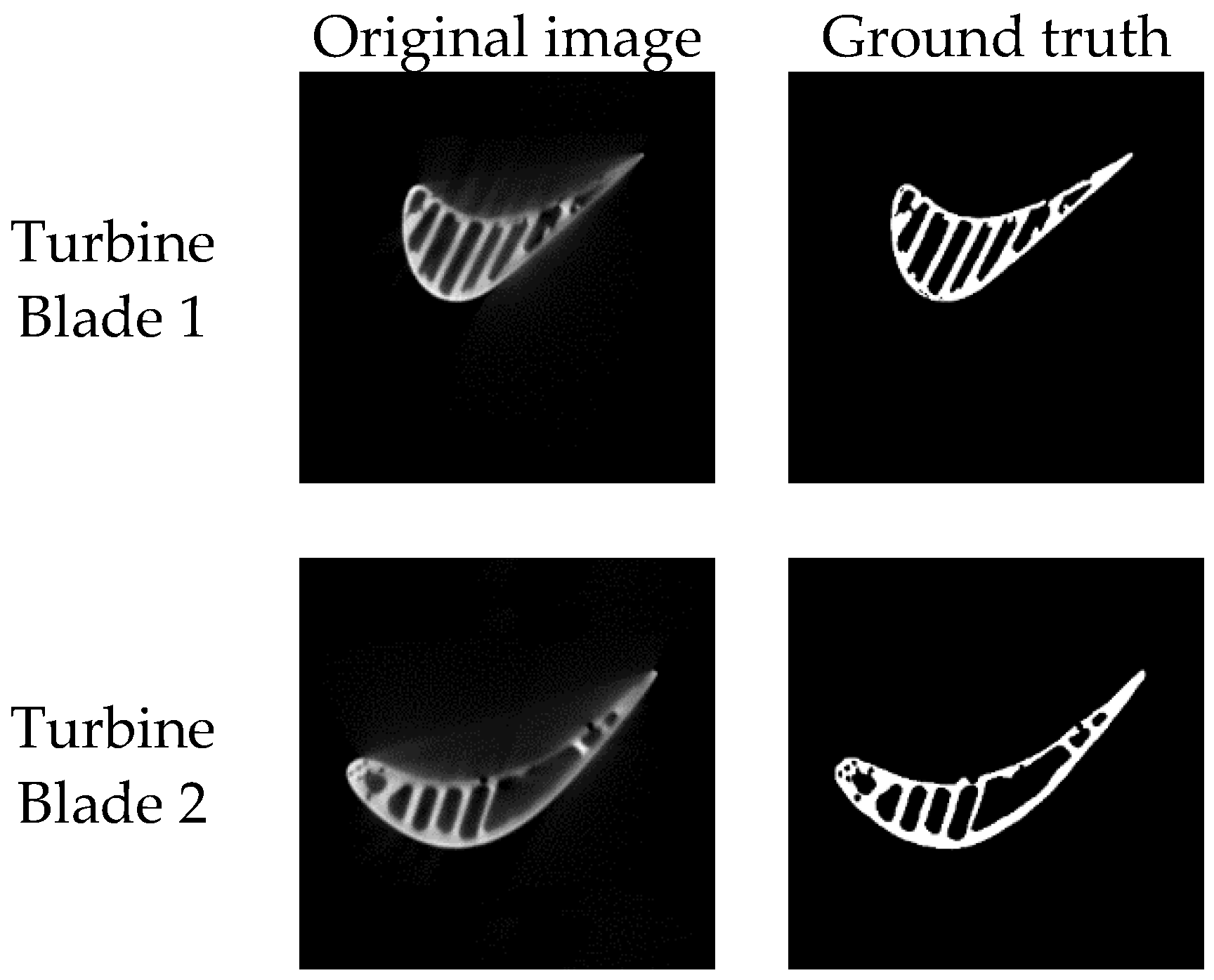
The original training data set contained a total of 493 slice images of two turbine blades, with the resolution cropped to 512 × 512. Another 180 and 30 slice images of these two turbine blades are used for validation and test, respectively. The ground truth of each image is manually labeled as follows:
(1) manually draw the contours of the turbine blade in the CT slice image;
(2) automatically fill in the area within the contour using the regional growth method.
Figure 5 shows the example of the original CT slice image and its manually labeled ground truth for both turbine blades.

2.3.2. Training Parameters

The training algorithm of the proposed network is “adam”, which could effectively decrease the learning rates of parameters with large parameter gradients and their squared values and increase the learning rates when gradients and squared values are small. The gradient moving average and decay rate of the squared gradient moving average of the training algorithm are set to 0.9 and 0.999, respectively. The initial learning rate is set to 0.001, and the epochs of the training process is 200. The minibatch size of the training is set to 8, and the validation frequency is set to every 30 iterations. The learning rate is reduced every ten epochs to improve the training effect by multiplying with a dropping factor of 0.95.

2.4. Performance Evaluation

The segmentation results are evaluated by the Jaccard similarity coefficient, as defined by the following equation:
Jaccard(A, T) = |A ∩ T|/|A ∪ T|
where A represents the segmentation result, T represents the ground truth, and ∩ and ∪ are the intersection and the union operations. || represents the number of pixels in the set. A higher Jaccard score means a better segmentation result.
Similarly, the dice similarity coefficient (DSC) is also used to evaluate the performance of the segmentation method, which can be expressed as:
DSC = 2|A ∩ T|/(|A| + |T|)
Another commonly used indicator is the BF score, i.e., how close the predicted boundary of an object matches the ground truth boundary. Compared with the Jaccard similarity coefficient, the BF score correlates better with human qualitative assessment. The BF score is defined as follows:
BF-Score = 2 × precision × recall/(recall + precision)
where precision is the fraction of detections that are true positives rather than false positives, while recall refers to the fraction of true positives that are detected rather than missed. Assuming TP, FP, FN, and TN represent the true positive, false positive, false negative, and true negative of the segmentation results, the precision = TP/(TP + FP), recall = TP/(TP + FN).

3. Results and Discussion

3.1. Segmentation Results

To demonstrate the effectiveness of the proposed method, it was compared with adaptively regularized kernel-based FCM (ARKFCM) [44], DRLSE [45], MAXENTROY [46], EM/MPM [47], continuous max-flow (CMF) [48], and OTSU [12]. MAXENTROPY, CMF, and OTSU methods are parameterless. Parameters of ARKFCM, DRLSE, and EM/MPM are listed in Table 1.
Our proposed method is compared with the conventional U-net, the dual-frame U-net [29], and the mU-net [37] approaches. The experimental results are depicted in Figure 6. In addition, a quantitative analysis of the experiments is listed in Table 2.
It can be known from Figure 6 that our proposed approach realized the best segmentation results compared with mathematical model-based segmentation methods and other U-net architectures. The ARKFCM method failed to segment the low contrast detail in the basin and the exhaust edge of both hollow turbine blades. In addition, small film cooling holes in the leading edges were also not segmented. For the DRLSE method, the target pixels on the edge of the hollow turbine blade are more likely to be mistakenly identified as the background, resulting in a certain dilation of the entire target object compared to the ground truth. Compared with the DRLSE method, the object dilation caused by this mis-segmentation is more obvious in the CMF method. Excessive dilation can cause severe deformation of the target, affecting the accuracy of subsequent measurements and registrations of the workpiece. Furthermore, the CMF method also failed in segmenting details in the blade basin and exhaust edge, as well as small film cooling holes scattered in the blade’s leading edge. The segmentation results of the EM/MPM and the MAXENTROPY methods were also ineffective, i.e., dilated edges, lack of details in low-contrast blade basin, and not segmented film cooling holes all appeared in both hollow turbine blades. For the Otsu method, the main issue was that the accuracy was not high, i.e., the edge details and film cooling holes were not successfully identified.
Compared with model-based segmentation methods, the comparison U-net architectures and our proposed enhanced U-net realized higher segmentation accuracies and details. The conventional U-net has a good segmentation effect in target with fewer artifacts and small details with good grayscale distribution, such as film cooling holes in the leading edge. However, it failed to segment small details with low contrast and artifacts, especially in the film cooling holes in the low-contrast leading edge and basin, as depicted in the red rectangle in Figure 6. Compared with dual-frame U-net and mU-net architectures, our proposed approach achieved better performance in segmentation accuracy and edge continuity. In fact, it is difficult for nonprofessionals to distinguish whether these pixels belong to the background or the target. The reason for this problem in conventional U-net is that its receptive field is not large enough. Simply increasing the depth of the network cannot improve the segmentation effect of tiny details with low contrast and artifacts. Therefore, this paper tried to increase the receptive field of the conventional U-net by using multiscale original images as input and adopting the dense block and residual path in the skip connection without increasing the depth of the network, thereby increasing the segmentation effect of indistinguishable details in the hollow turbine blade CT images caused by low contrast and artifacts.
To quantitatively analyze the segmentation effects of the proposed approach and the comparison methods, the BF score, the Jaccard, and the DSC indexes of each segmentation result are listed in Table 2. For the segmentation samples of 1#102, 1#111, 1#113, and 2#741, our proposed approach achieved the highest BF scores, Jaccard, and DSC indexes among all the segmentation results. Although the conventional U-net realized the highest BF score of sample 2#743, it is only 0.001 higher than our proposed approach. Moreover, the smoothness of the object contour in the segmentation results of the conventional U-net is not as good as our proposed method. More importantly, the conventional U-net cannot segment the film cooling holes in the leading edge in both samples, demonstrating our proposed approach’s superiority. The statistical T-test differences between each comparison method and our proposed approach are listed in Table 3. It can be known from Table 3 that the p-values of traditional mathematical model-based methods are all smaller than 0.01, which means that our proposed approach outperforms these traditional methods. For conventional U-net, its p-values of Jaccard and DSC indexes are smaller than 0.05, which means that our proposed approach performs better than the conventional U-net. For dual-frame U-net and mU-net, their p-values range 0.45~0.98, which means that our proposed enhanced U-net can achieve a slightly enhanced segmentation effect. It is worth noting that the p-value of dual-frame U-net is higher than that of mU-net, which indicates that the performance of dual-frame U-net is closer to our proposed approach.

3.2. Analysis of the Proposed Architecture

3.2.1. Ablation Experiments

In order to quantitatively analyze the effectiveness of our proposed approach, four groups of ablation experiments were conducted in this paper to verify the improvement effect of multi-input, dense block, focal loss function, and residual path in the skip connection on turbine blade segmentation, respectively. The results are listed in Table 4. It can be known from Table 4 that the dense block and the multi-input modifications played more critical roles in the improvement of the segmentation results. The residual path and focal loss function modifications further enhanced the effect of the proposed architecture.

3.2.2. Processing Time

To study the segmentation efficiency of the proposed approach, the running time of the proposed approach and all comparison methods are listed in Table 5.
It can be known from Table 5 that the deep learning-based methods consumed much less time compared with conventional model-based methods. The most time-saving MAXENTROPY method is still an order of magnitude more than the deep learning-based approaches. For the U-net architecture, the more layers the network has, the more segmentation time it consumes. However, it is worth noting that deep learning algorithms run on GPU, while conventional model-based methods run on CPU. This difference also determines that the efficiency of these methods is only horizontally comparable.

3.2.3. Robustness of the Proposed Architecture

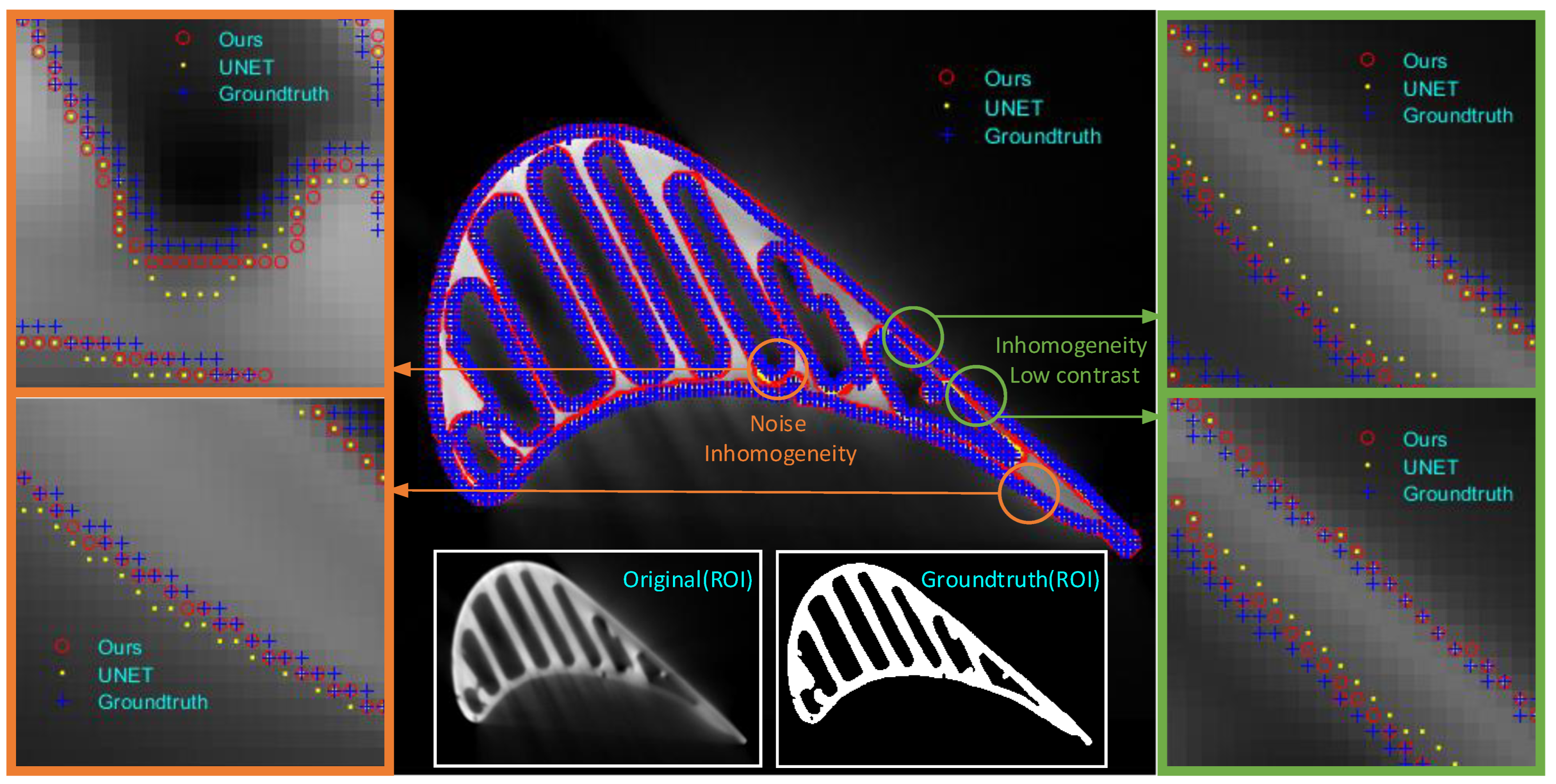
To study the robustness of the proposed approach, this paper evaluated it on sample 1#268 with severe inhomogeneity, noise, and low contrast. The comparison results with conventional U-net are depicted in Figure 7.
It can be known from Figure 7 that the proposed approach can realize a better segmentation effect compared with conventional U-net in terms of low-quality images. For the region with insufficient contrast, the conventional U-net can easily cause mis-segmentation. For example, in the blade tail, the severe low contrast and inhomogeneity directly affect the U-net judgment of the edge contour. Pixels that originally belonged to the object were mis-segmented as the background.
In summary, the deep learning approach outperforms conventional model-based methods in segmentation accuracy and protecting tiny details. The essential reason is that, compared with conventional mathematical model-based segmentation methods, the deep neural network-based approach has a good learning effect on the continuity between slice images. This is because the physical distance between two adjacent layers is very small (often around 0.1 mm), so the interlayer variation of the sliced image is relatively small. When this layer is affected by uneven contrast or artifacts, conventional mathematical model algorithms are prone to mis-segmentation. The deep neural network not only learns the association between the real image of the current layer and the corresponding ground truth but also the real image information of adjacent layers. Therefore, when an ambiguous structure only exists in a few layers, it will not have a large impact on the convergence effect of the deep neural network.

3.3. Limitations

Due to the particular structure and material characteristics of the aeroengine turbine blade, its CT images have very obvious artifacts and inhomogeneity at the edges and inner cavities. Therefore, the conventional model-based image segmentation methods are often unsatisfactory for the CT image of the turbine blade, where the loss of details and mis-segmentation often occur. The use of supervised deep learning methods can effectively improve the segmentation effect of turbine blade CT images. The experimental results of this paper have demonstrated that the deep learning method has completely surpassed the conventional model method, whether in terms of processing speed or segmentation accuracy. In this paper, some improvements have been made on the basis of the conventional U-net architecture. Compared with the conventional U-net, the segmentation accuracy has been improved to a certain extent even under the influence of artifacts and inhomogeneity. However, due to a large number of tiny air film cooling holes in the turbine blades and the complex exhaust edges at the tail, it is still difficult to acquire precise details, even with the help of deep learning approaches. These difficult-to-divide air cooling film holes and exhaust edges are essential for turbine blades, which play an important role in the heat dissipation of turbine blades under extremely high temperatures and high-pressure conditions. Therefore, further efforts are needed to improve the segmentation accuracy of turbine blade details.

4. Conclusions

This paper presented an enhanced U-net for the segmentation of the aeroengine hollow turbine blade. The enhanced U-net is modified based on the conventional U-net architecture, where the multiscale input, dense block, focal loss function, and residual path in the skip connection are added to improve the receptive field of the network without increasing its longitudinal depth. Experiments were conducted based on a set of ICT slice images of two practical hollow turbine blades, namely, the CFM56-7BE and Pratt & Whitney F100 blades. The experimental results indicate that our proposed approach has the best segmentation results in terms of segmentation accuracy and protection of tiny details with low contrast and artifacts compared with typical model-based algorithms and the conventional U-net. Future work of this paper will focus on improving the segmentation accuracy of tiny objects in the blade, such as film cooling holes and exhaust edges, etc.

Author Contributions

Conceptualization, J.Z. and Y.S.; methodology, J.Z.; validation, J.Z., C.T., and Y.S. formal analysis, C.T. and C.W.; investigation, C.T. and M.F.; resources, J.Z.; data curation, C.W.; writing—original draft preparation, J.Z.; writing—review and editing, Y.S.; supervision, M.F.; project administration, Y.S.; funding acquisition, J.Z. and Y.S. All authors have read and agreed to the published version of the manuscript.

Funding

This research was funded by National Natural Science Foundation of China, grant number 62101086, 62003060, 52005070; China Postdoctoral Science Foundation, grant number 2021M693769; Scientific and Technological Research Program of Chongqing Municipal Education Commission, grant number KJQN202100648; Natural Science Foundation of Chongqing, China, grant number cstc2021jcyj-bsh0180, CSTB2022NSCQ-MSX1297, cstc2020jcyj-msxmX0886.

Data Availability Statement

Not applicable.

Conflicts of Interest

The authors declare no conflict of interest.

References

  1. Dong, Y.W.; Li, X.L.; Zhao, Q.; Yang, J.; Dao, M. Modeling of shrinkage during investment casting of thin-walled hollow turbine blades. J. Mater. Process. Technol. 2017, 244, 190–203. [Google Scholar] [CrossRef]
  2. Ohtake, Y.; Suzuki, H. Edge detection based multi-material interface extraction on industrial CT volumes. Sci. China Ser. F Inf. Sci. 2013, 56, 1–9. [Google Scholar] [CrossRef]
  3. Ciliberti, G.A.; Janello, P.; Jahnke, P.; Keuthage, L. Potentials of Full-Vehicle CT Scans Within the Automotive Industry. In Proceedings of the 19th World Conference on Nondestructive Testing (WCNDT 2016), Munich, Germany, 13–17 June 2016. [Google Scholar]
  4. Qian, X.; Wang, J.; Guo, S.; Li, Q. An active contour model for medical image segmentation with application to brain CT image. Med. Phys. 2013, 40, 021911. [Google Scholar] [CrossRef] [PubMed] [Green Version]
  5. Ketcham, R.A.; Carlson, W.D. Acquisition, optimization and interpretation of X-ray computed tomographic imagery: Applications to the geosciences. Comput. Geosci. 2001, 27, 381–400. [Google Scholar] [CrossRef]
  6. Lee, J.H.; Lee, J.M.; Park, J.W.; Moon, Y.S. Efficient algorithms for automatic detection of cracks on a concrete bridge. In Proceedings of the 23rd International Technical Conference on Circuits/Systems, Computers and Communications, Shimonoseki, Japan, 6–9 July 2008; pp. 1213–1216. [Google Scholar]
  7. Zheng, J.; Zhang, D.; Huang, K.; Sun, Y. Cone-Beam Computed Tomography Image Pretreatment and Segmentation. In Proceedings of the International Symposium on Computational Intelligence and Design, Hangzhou, China, 8–9 December 2018; pp. 25–28. [Google Scholar]
  8. Ayala, H.V.H.; Santos, F.M.d.; Mariani, V.C.; Coelho, L.d.S. Image thresholding segmentation based on a novel beta differential evolution approach. Expert Syst. Appl. 2015, 42, 2136–2142. [Google Scholar] [CrossRef]
  9. Alaknanda; Anand, R.S.; Kumar, P. Flaw detection in radiographic weld images using morphological approach. Ndt E Int. 2006, 39, 29–33. [Google Scholar] [CrossRef]
  10. Zhang, K.; Zhang, L.; Song, H.; Zhou, W. Active contours with selective local or global segmentation: A new formulation and level set method. Image Vis. Comput. 2010, 28, 668–676. [Google Scholar] [CrossRef]
  11. Zheng, J.; Zhang, D.; Huang, K.; Sun, Y. Adaptive image segmentation method based on the fuzzy c-means with spatial information. Iet Image Process. 2017, 12, 785–792. [Google Scholar] [CrossRef]
  12. Zheng, J.; Zhang, D.; Huang, K.; Sun, Y.; Tang, S. Adaptive windowed range-constrained Otsu method using local information. J. Electron. Imaging 2016, 25, 013034. [Google Scholar] [CrossRef]
  13. Alaknanda; Anand, R.S.; Kumar, P. Flaw detection in radiographic weldment images using morphological watershed segmentation technique. Ndt E Int. 2009, 42, 2–8. [Google Scholar] [CrossRef]
  14. Prathusha, P.; Jyothi, S. A Novel Edge Detection Algorithm for Fast and Efficient Image Segmentation; Springer: Singapore, 2018; pp. 283–291. [Google Scholar]
  15. Li, Y.; Cao, G.; Yu, Q.; Li, X. Fast and Robust Active Contours Model for Image Segmentation. Neural Process. Lett. 2019, 49, 431–452. [Google Scholar] [CrossRef]
  16. Dellepiane, S.G.; Nardotto, S. Fuzzy Image Segmentation: An Automatic Unsupervised Method; Springer International Publishing: Berlin/Heidelberg, Germany, 2014; pp. 65–88. [Google Scholar]
  17. Lecun, Y.; Bengio, Y.; Hinton, G. Deep learning. Nature 2015, 521, 436–444. [Google Scholar] [CrossRef] [PubMed]
  18. Guo, Y.; Liu, Y.; Georgiou, T.; Lew, M.S. A review of semantic segmentation using deep neural networks. Int. J. Multimed. Inf. Retr. 2018, 7, 87–93. [Google Scholar] [CrossRef] [Green Version]
  19. Minaee, S.; Boykov, Y.; Porikli, F.; Plaza, A.; Kehtarnavaz, N.; Terzopoulos, D. Image Segmentation Using Deep Learning: A Survey. IEEE Trans. Pattern Anal. Mach. Intell. 2022, 44, 3523–3542. [Google Scholar] [CrossRef] [PubMed]
  20. Long, J.; Shelhamer, E.; Darrell, T. Fully convolutional networks for semantic segmentation. In Proceedings of the 2015 IEEE Conference on Computer Vision and Pattern Recognition (CVPR), Boston, MA, USA, 7–12 June 2015; pp. 3431–3440. [Google Scholar]
  21. Noh, H.; Hong, S.; Han, B. Learning Deconvolution Network for Semantic Segmentation. In Proceedings of the 2015 IEEE International Conference on Computer Vision (ICCV), Santiago, Chile, 7–13 December 2015; pp. 1520–1528. [Google Scholar]
  22. Lin, T.Y.; Dollár, P.; Girshick, R.; He, K.; Hariharan, B.; Belongie, S. Feature Pyramid Networks for Object Detection. In Proceedings of the 2017 IEEE Conference on Computer Vision and Pattern Recognition (CVPR), Honolulu, HI, USA, 21–26 July 2017; pp. 936–944. [Google Scholar]
  23. Ren, S.; He, K.; Girshick, R.; Sun, J. Faster R-CNN: Towards Real-Time Object Detection with Region Proposal Networks. IEEE Trans. Pattern Anal. Mach. Intell. 2017, 39, 1137–1149. [Google Scholar] [CrossRef] [PubMed] [Green Version]
  24. Chen, L.C.; Papandreou, G.; Kokkinos, I.; Murphy, K.; Yuille, A.L. DeepLab: Semantic Image Segmentation with Deep Convolutional Nets, Atrous Convolution, and Fully Connected CRFs. IEEE Trans. Pattern Anal. Mach. Intell. 2018, 40, 834–848. [Google Scholar] [CrossRef] [PubMed] [Green Version]
  25. Visin, F.; Romero, A.; Cho, K.; Matteucci, M.; Ciccone, M.; Kastner, K.; Bengio, Y.; Courville, A. ReSeg: A Recurrent Neural Network-Based Model for Semantic Segmentation. In Proceedings of the 2016 IEEE Conference on Computer Vision and Pattern Recognition Workshops (CVPRW), Las Vegas, NV, USA, 26 June–1 July 2016; pp. 426–433. [Google Scholar]
  26. Chen, L.C.; Yang, Y.; Wang, J.; Xu, W.; Yuille, A.L. Attention to Scale: Scale-Aware Semantic Image Segmentation. In Proceedings of the 2016 IEEE Conference on Computer Vision and Pattern Recognition (CVPR), Las Vegas, NV, USA, 27–30 June 2016; pp. 3640–3649. [Google Scholar]
  27. Souly, N.; Spampinato, C.; Shah, M. Semi Supervised Semantic Segmentation Using Generative Adversarial Network. In Proceedings of the 2017 IEEE International Conference on Computer Vision (ICCV), Venice, Italy, 22–29 October 2017; pp. 5689–5697. [Google Scholar]
  28. Falk, T.; Mai, D.; Bensch, R.; Çiçek, Ö.; Abdulkadir, A.; Marrakchi, Y.; Böhm, A.; Deubner, J.; Jäckel, Z.; Seiwald, K.; et al. U-Net: Deep learning for cell counting, detection, and morphometry. Nat. Methods 2019, 16, 67–70. [Google Scholar] [CrossRef]
  29. Han, Y.; Ye, J.C. Framing U-Net via Deep Convolutional Framelets: Application to Sparse-View CT. IEEE Trans. Med. Imaging 2018, 37, 1418–1429. [Google Scholar] [CrossRef] [Green Version]
  30. Yin, X.-X.; Sun, L.; Fu, Y.; Lu, R.; Zhang, Y. U-Net-Based Medical Image Segmentation. J. Healthc. Eng. 2022, 2022, 1–16. [Google Scholar] [CrossRef]
  31. Baltruschat, I.M.; Ćwieka, H.; Krüger, D.; Zeller-Plumhoff, B.; Schlünzen, F.; Willumeit-Römer, R.; Moosmann, J.; Heuser, P. Scaling the U-net: Segmentation of biodegradable bone implants in high-resolution synchrotron radiation microtomograms. Sci. Rep. 2021, 11, 24237. [Google Scholar] [CrossRef]
  32. Ghosh, S.; Chaki, A.; Santosh, K. Improved U-Net architecture with VGG-16 for brain tumor segmentation. Phys. Eng. Sci. Med. 2021, 44, 703–712. [Google Scholar] [CrossRef] [PubMed]
  33. Khaled, R.; Vidal, J.; Vilanova, J.C.; Martí, R. A U-Net Ensemble for breast lesion segmentation in DCE MRI. Comput. Biol. Med. 2022, 140, 105093. [Google Scholar] [CrossRef] [PubMed]
  34. Li, A.C.; Vyas, S.; Lin, Y.H.; Huang, Y.Y.; Huang, H.M.; Luo, Y. Patch-Based U-Net Model for Isotropic Quantitative Differential Phase Contrast Imaging. IEEE Trans. Med. Imaging 2021, 40, 3229–3237. [Google Scholar] [CrossRef]
  35. Lee, S.A.; Konofagou, E.E. FUS-Net: U-Net-Based FUS Interference Filtering. IEEE Trans. Med. Imaging 2022, 41, 915–924. [Google Scholar] [CrossRef] [PubMed]
  36. Rocha, J.; Cunha, A.; Mendonça, A.M. Conventional Filtering Versus U-Net Based Models for Pulmonary Nodule Segmentation in CT Images. J. Med. Syst. 2020, 44, 1–8. [Google Scholar] [CrossRef]
  37. Seo, H.; Huang, C.; Bassenne, M.; Xiao, R.; Xing, L. Modified U-Net (mU-Net) With Incorporation of Object-Dependent High Level Features for Improved Liver and Liver-Tumor Segmentation in CT Images. IEEE Trans. Med. Imaging 2020, 39, 1316–1325. [Google Scholar] [CrossRef] [PubMed] [Green Version]
  38. Man, Y.; Huang, Y.; Feng, J.; Li, X.; Wu, F. Deep Q Learning Driven CT Pancreas Segmentation With Geometry-Aware U-Net. IEEE Trans. Med. Imaging 2019, 38, 1971–1980. [Google Scholar] [CrossRef] [Green Version]
  39. Hiasa, Y.; Otake, Y.; Takao, M.; Ogawa, T.; Sugano, N.; Sato, Y. Automated Muscle Segmentation from Clinical CT Using Bayesian U-Net for Personalized Musculoskeletal Modeling. IEEE Trans. Med. Imaging 2020, 39, 1030–1040. [Google Scholar] [CrossRef] [Green Version]
  40. He, K.; Lian, C.; Zhang, B.; Zhang, X.; Cao, X.; Nie, D.; Gao, Y.; Zhang, J.; Shen, D. HF-UNet: Learning Hierarchically Inter-Task Relevance in Multi-Task U-Net for Accurate Prostate Segmentation in CT Images. IEEE Trans. Med. Imaging 2021, 40, 2118–2128. [Google Scholar] [CrossRef]
  41. Wang, B.; Chen, Z.; Dewulf, W.; Pauwels, R.; Yao, Z.; Hou, Q.; Xiao, Y. U-net-based blocked artifacts removal method for dynamic computed tomography. Appl. Opt. 2019, 58, 3748. [Google Scholar] [CrossRef]
  42. Li, X.; Song, W.; Gao, D.; Gao, W.; Wang, H. Training a U-Net based on a random mode-coupling matrix model to recover acoustic interference striations. J. Acoust. Soc. Am. 2020, 147, EL363–EL369. [Google Scholar] [CrossRef] [PubMed] [Green Version]
  43. Wang, W.; Li, Q.; Xiao, C.; Zhang, D.; Miao, L.; Wang, L. An Improved Boundary-Aware U-Net for Ore Image Semantic Segmentation. Sensors 2021, 21, 2615. [Google Scholar] [CrossRef] [PubMed]
  44. Cherfa, I.; Mokraoui, A.; Mekhmoukh, A.; Mokrani, K. Adaptively Regularized Kernel-Based Fuzzy C-Means Clustering Algorithm Using Particle Swarm Optimization for Medical Image Segmentation. In Proceedings of the 2020 Signal Processing: Algorithms, Architectures, Arrangements, and Applications (SPA), Poznan, Poland, 23–25 September 2020; pp. 24–29. [Google Scholar]
  45. Wang, D. Extremely optimized DRLSE method and its application to image segmentation. IEEE Access 2019, 7, 119603–119619. [Google Scholar] [CrossRef]
  46. Merzougui, M.; El Allaoui, A. Region growing segmentation optimized by evolutionary approach and Maximum Entropy. Procedia Comput. Sci. 2019, 151, 1046–1051. [Google Scholar] [CrossRef]
  47. Masuda, Y.; Tateyama, T.; Xiong, W.; Zhou, J.; Wakamiya, M.; Kanasaki, S.; Furukawa, A.; Chen, Y.W. Liver tumor detection in CT images by adaptive contrast enhancement and the EM/MPM algorithm. In Proceedings of the 2011 18th IEEE International Conference on Image Processing, Brussels, Belgium, 11–14 September 2011; pp. 1421–1424. [Google Scholar]
  48. Wu, M.; Fan, W.; Chen, Q.; Du, Z.; Li, X.; Yuan, S.; Park, H. Three-dimensional continuous max flow optimization-based serous retinal detachment segmentation in SD-OCT for central serous chorioretinopathy. Biomed. Opt. Express 2017, 8, 4257–4274. [Google Scholar] [CrossRef]
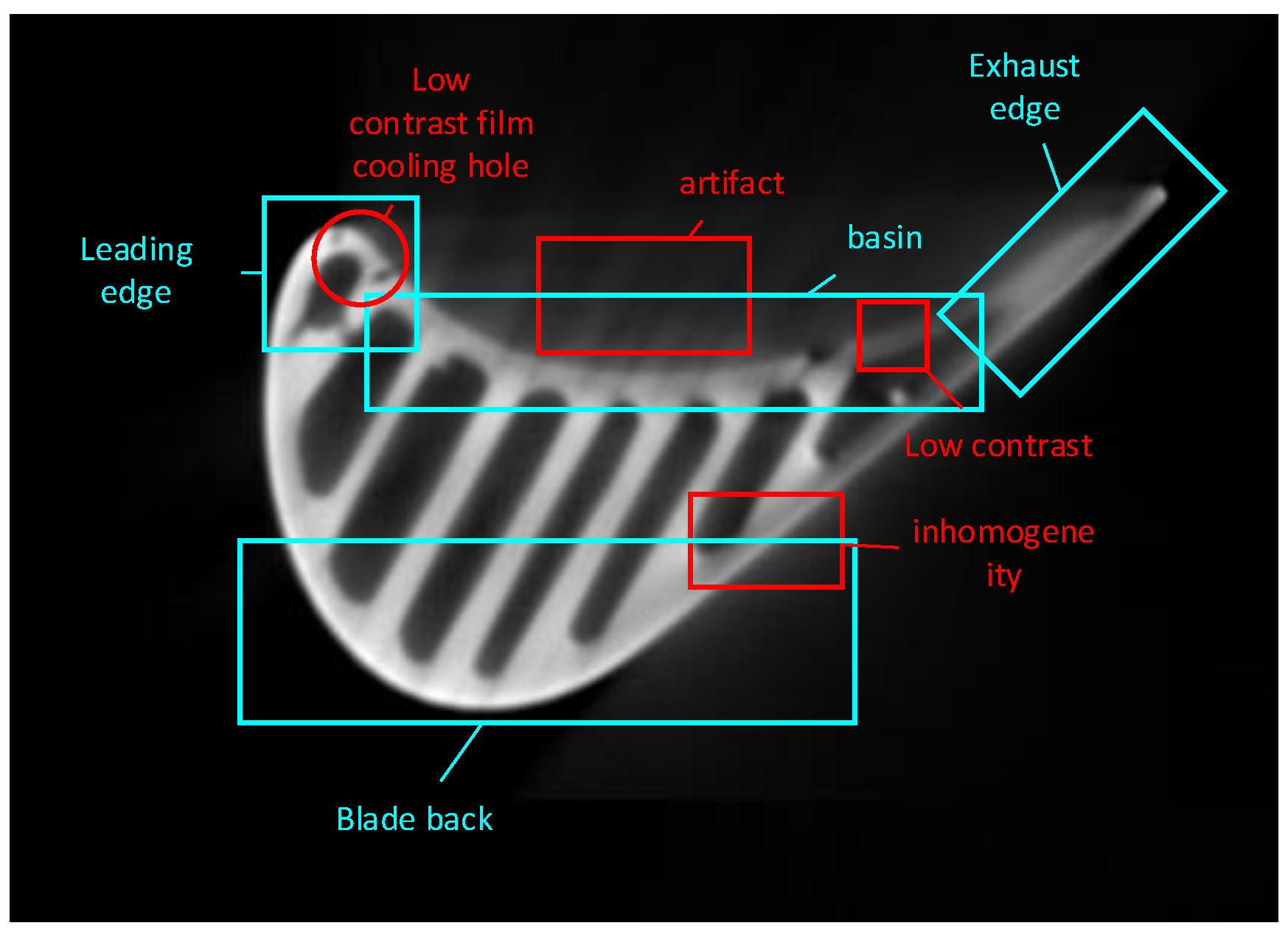
Figure 1. ICT image of the hollow turbine blade.
Mathematics 10 04230 g001
Figure 2. The working principle of the ICT system.
Mathematics 10 04230 g002
Figure 3. Turbine blades: (a) CFM56-7BE aeroengine and (b) Pratt & Whitney F100 aeroengine.
Mathematics 10 04230 g003
Figure 4. Structure of the enhanced U-net.
Mathematics 10 04230 g004
Figure 5. Training data samples of two turbine blades.
Mathematics 10 04230 g005
Figure 6. Experimental results of the proposed method, ARKFCM, DRLSE, MAXENTROPY, EM/MPM, CMF, OTSU, conventional U-net, dual-frame U-net and mU-net.
Mathematics 10 04230 g006
Figure 7. Robustness analysis of the proposed approach on the low-quality sample 1#268.
Mathematics 10 04230 g007
Table 1. Parameters of the comparing methods.
Samples1#1021#1111#1132#7402#7412#743
Methods
ARKFCMwinSize = 45;
cNum = 2;
opt = ‘average’
winSize = 31;
cNum = 2;
opt = ‘median’
winSize = 41;
cNum = 2;
opt = ‘median’
winSize = 27;
cNum = 2;
opt = ‘weighted’
winSize = 15;
cNum = 2;
opt = ‘weighted’
winSize = 16;
cNum = 2;
opt = ‘weighted’
DRLSEsigma = 45;
iter_outer = 60;
iter_inner = 10;
timestep = 0.1;
c0 = 1;
mu = 1;
sigma = 35;
iter_outer = 40;
iter_inner = 10;
timestep = 0.1;
c0 = 1;
mu = 0.1;
sigma = 35;
iter_outer = 50;
iter_inner = 10;
timestep = 0.1;
c0 = 1;
mu = 1;
sigma = 21;
iter_outer = 26;
iter_inner = 10;
timestep = 0.1;
c0 = 1;
mu = 1;
sigma = 21;
iter_outer = 26;
iter_inner = 10;
timestep = 0.1;
c0 = 1;
mu = 1;
sigma = 21;
iter_outer = 26;
iter_inner = 10;
timestep = 0.1;
c0 = 1;
mu = 1;
EM/MPMregions = 2;
steps = 10;
mpmSteps = 1;
coolMax = 1.2
coolInc = 0.25
regions = 2;
steps = 16;
mpmSteps = 10;
coolMax = 1.2
coolInc = 0.025
regions = 2;
steps = 18;
mpmSteps = 1;
coolMax = 1.2
coolInc = 0.025
regions = 2;
steps = 1;
mpmSteps = 1;
coolMax = 1.2
coolInc = 0.025
regions = 2;
steps = 1;
mpmSteps = 5;
coolMax = 1.2
coolInc = 0.025
regions = 2;
steps = 10;
mpmSteps = 8;
coolMax = 1.2
coolInc = 0.025
Table 2. Performance of the proposed approach and the comparison methods.
Evaluation IndexMethodsExperimental Results
1#1021#1111#1132#7402#7412#743
BF ScoreARKFCM0.98900.98890.98760.98010.98040.9863
CMF0.94030.90960.90920.81690.81270.8585
DRLSE0.99840.98180.98610.97130.96510.9793
EM/MPM0.99280.98760.98620.97690.97680.9824
MAXENTROPY0.98890.98720.98250.92910.91530.9177
OTSU0.99520.98990.98760.97990.98000.9858
Conventional U-net1.00001.00001.00000.99600.99641.0000
Proposed1.00001.00001.00000.99650.99690.9990
Dual-Frame U-net1.00001.00001.00000.99630.99670.9995
mU-net1.00001.00001.00000.99700.99670.9995
JaccardARKFCM0.81830.76220.79040.79640.79240.8121
CMF0.61970.56040.58650.58650.58620.6176
DRLSE0.77110.70130.74010.75140.74910.7815
EM/MPM0.81220.74250.77110.77200.76650.7916
MAXENTROPY0.74250.69730.72090.68530.67890.7012
OTSU0.80920.73880.76780.76770.76340.7879
Conventional U-net0.94970.93110.93130.94230.94180.9472
Proposed0.95400.93920.94230.95470.95540.9592
Dual-Frame U-net0.94850.93910.94040.95530.95500.9590
mU-net0.94740.93830.93770.95340.95180.9550
DSCARKFCM0.90010.86510.88290.88670.88420.8963
CMF0.76520.71830.73940.73940.73910.7636
DRLSE0.87080.82440.85060.85810.85660.8774
EM/MPM0.89640.85220.87080.87130.86780.8837
MAXENTROPY0.85220.82170.83780.81330.80870.8244
OTSU0.89450.84980.86870.86860.86580.8814
Conventional U-net0.97420.96430.96440.97030.97000.9729
Proposed0.97650.96860.97030.97680.97720.9792
Dual-Frame U-net0.97360.96860.96930.97710.97700.9791
mU-net0.97300.96820.96780.97610.97530.9770
Table 3. Statistical T-test difference between each comparison method and our proposed approach.
MethodARKFCMCMFDRLSEEM/MPMMAXENTROPYOTSUConventional U-netDual-Frame U-netmU-net
p-Value
p-BF2.27 × 10−50.0001940.0032790.0002240.0120900.0005981.0000000.9867370.888246
p-Jaccard6.34 × 10−95.19 × 10−121.05 × 10−89.79 × 10−93.37 × 10−108.6 × 10−90.0497920.7967740.452846
p-DSC1.21 × 10−82.79 × 10−112.9 × 10−82.04 × 10−89.45 × 10−101.78 × 10−80.0504540.7996910.453197
Table 4. Ablation experiments of the proposed approach.
Evaluation
Index
MethodsExperimental Results
1#1021#1111#1132#7402#7412#743
BF ScoreDense Block + U-net1.00001.00001.00000.99610.99680.9991
Multi Input + U-net1.00001.00001.00000.99640.99670.9991
Focal Loss + U-net1.00001.00000.99980.99670.99670.9998
Residual Path + U-net1.00001.00001.00000.99700.99670.9995
Conventional U-net1.00001.00001.00000.99600.99641.0000
Proposed1.00001.00001.00000.99650.99690.9990
JaccardDense Block + U-net0.94920.93970.94060.95350.95300.9578
Multi Input + U-net0.94870.93970.94190.95570.95400.9600
Focal Loss + U-net0.93290.93370.92730.95330.95140.9502
Residual Path + U-net0.94740.93830.93770.95340.95180.9550
Conventional U-net0.9497 0.9311 0.9313 0.9423 0.9418 0.9472
Proposed0.95400.93920.94230.95470.95540.9592
DSCDense Block + U-net0.97390.96890.96940.97620.97590.9784
Multi-Input + U-net0.97370.96890.97010.97730.97650.9796
Focal Loss + U-net0.96530.96570.96230.97610.97510.9745
Residual Path + U-net0.97300.96820.96780.97610.97530.9770
Conventional U-net0.97420.96430.96440.97030.97000.9729
Proposed0.97650.96860.97030.97680.97720.9792
Table 5. Processing time of the proposed approach and the comparison methods.
MethodsARKFCMCMFDRLSEEM/MPMMAXENTROPYOTSUU-netProposedmU-netDual-Frame U-net
Samples
1#1026.003 s0.425 s134.397 s0.904 s0.367 s0.128 s0.0315 s0.0810 s0.0418 s0.0304 s
1#1115.927 s0.435 s59.553 s0.706 s0.360 s0.073 s0.0325 s0.0811 s0.0428 s0.0299 s
1#1136.697 s0.438 s76.094 s0.737 s0.327 s0.082 s0.0319 s0.0806 s0.0423 s0.0294 s
2#7406.117 s0.504 s25.223 s0.906 s0.320 s0.086 s0.0330 s0.0810 s0.0418 s0.0295 s
2#7415.902 s0.471 s22.218 s0.935 s0.297 s0.086 s0.0294 s0.0810 s0.0388 s0.0301 s
2#7435.899 s0.514 s22.111 s0.759 s0.424 s0.104 s0.0292 s0.0807 s0.0404 s0.0296 s
Publisher’s Note: MDPI stays neutral with regard to jurisdictional claims in published maps and institutional affiliations.