Article

Population-Based Meta-Heuristic Algorithms for Integrated Batch Manufacturing and Delivery Scheduling Problem

Department of Industrial and Management Engineering, Incheon National University, 119, Academy-ro, Yeonsu-gu, Incheon 22012, Korea
*
Author to whom correspondence should be addressed.
Mathematics 2022, 10(21), 4127; https://doi.org/10.3390/math10214127
Submission received: 11 October 2022 / Revised: 27 October 2022 / Accepted: 2 November 2022 / Published: 4 November 2022
(This article belongs to the Topic Soft Computing)

Abstract

:
This paper addresses an integrated scheduling problem of batch manufacturing and delivery processes with a single batch machine and direct-shipping trucks. In the manufacturing process, some jobs in the same family are simultaneously processed as a production batch in a single machine. The batch production time depends only on the family type assigned to the production batch and it is dynamically adjusted by batch deterioration and rate-modifying activities. Each job after the batch manufacturing is reassigned to delivery batches. In the delivery process, each delivery batch is directly shipped to the corresponding customer. The delivery time of delivery batches is determined by the distance between the manufacturing site and customer location. The total volume of jobs in each production or delivery batch must not exceed the machine or truck capacity. The objective function is to minimize the total tardiness of jobs delivered to customers with different due dates. To solve the problem, a mixed-integer linear programming model to find the optimal solution for small problem instances is formulated and meta-heuristic algorithms to find effective solutions for large problem instances are presented. Sensitivity analyses are conducted to find the effect of problem parameters on the manufacturing and delivery time.

1. Introduction

Recently, many studies have been conducted on individual manufacturing and delivery problems, both of which are an important part of supply chain management (SCM). The methodologies for an integrated scheduling problem (ISP) generally provide better performance to improve the efficiency of the entire supply chain than individual manufacturing and delivery problems [1]. The study on ISPs is difficult even if ISPs provide better performance because of the complexity of the supply chain and the conflict of stakeholders in the supply chain. Nevertheless, ISPs are required for many sectors of industry such as ceramics, food, port cargo handling, and freight logistics [2]. In this study, we confine our study to ISPs regarding the manufacturing and delivery process. We apply the batch loading and scheduling problem (BLSP) in the manufacturing process [3] and the direct-shipping problem in the delivery process [1,4].
In the manufacturing process, jobs can be processed simultaneously on a batch processing machine, and a set of jobs that are processed simultaneously is called a production batch. The volumes of jobs are different. The total volume in a production batch must not exceed the machine capacity. Jobs with different families must not be assigned to the same production batch. The batch production time depends only on the family type assigned to the production batch. Furthermore, we consider deterioration and rate-modifying activities. In collaborative works between operators and machines, such as machining, assembling, and maintenance, the batch production time can increase due to operator fatigue or machine failure, where the increased portion of this batch production time is called deterioration. The recovery process from the deteriorated state to the original state is called rate-modifying activity (RMA) [5]. In this study, the batch production time increases in proportion to the interval between the recent RMA and the start time of the batch because we assume that the deterioration effect occurs linearly.
In the delivery process, each job after batch manufacturing is reassigned to delivery batches. The delivery batches are directly shipped by fixed numbers of homogeneous trucks. In this study, we consider that the delivery batch is independent of the production batch. The total volume in a delivery batch must not exceed the truck capacity. Jobs from different customers must not be assigned to the same delivery batch. The truck can deliver only one delivery batch at a time. The truck leaving the factory returns immediately after shipping the delivery batch to the customer. The delivery time including return time depends only on the customer of that particular delivery batch. The objective function is minimizing the total tardiness of jobs delivered to customers with different due dates.
Figure 1 describes a Gantt chart example for the presented ISP. The number of jobs, families, and customers are 5, 2, and 2, respectively. Jobs 1 and 2 belong to Family 1 and Jobs 3, 4, and 5 belong to Family 2. Jobs 1, 3, and 5 are requested from Customer 1, and Jobs 2 and 4 are requested from Customer 2. The production time for the family and the delivery time for the customer are (50, 100) and (229, 161), respectively. The due date and volume of jobs are (264, 235, 401, 477, 459) and (5, 10, 7, 14, 10), respectively. The machine capacity, truck capacity, deterioration rate, and RMA processing time are 20, 20, 0.3, and 20, respectively. The jobs are assigned to production batches ( B M ) while keeping the constraints on the family compatibility and machine capacity. The production batches are sequenced with RMAs inserted between them. The production time of Batch 2 increases in proportion to the interval between the start time of Batches 2 and 1 due to deterioration. The original production time of Batch 2 is 100. The interval between the start time of Batches 2 and 1 is 50. The deterioration rate is 20. Thus, the production time of Batch 2 is 115 (=100 + 50 × 0.3). Assuming the RMA was performed before Batch 3 is processed, the deterioration for Batch 3 is restored and the batch production time is not increased. The manufacturing completion time of jobs is (50, 50, 165, 285, 165). Jobs that have been processed are assigned to delivery batches ( B D ) while keeping the constraints on the customer compatibility and the truck capacity. Truck 1 transports Batch 2 at time 279, but the manufacturing completion time of Job 4 is 285. Therefore, the waiting time is 6 (= 285 – 279) between Batches 2 and 3 in Truck 1. The completion time of jobs in the batches for the corresponding customer is (279, 211, 440, 446, 440). By comparing the due dates of each job, the total tardiness of each job is 54 (=15 + 0 + 39 + 0 + 0).

2. Literature Review

In this section, we survey studies on ISPs, including batch processing. For ISPs including deterioration or RMA, we focus on their scheme.
For ISPs with a direct-shipping method, Liu [6] dealt with a two-stage delivery problem. The first stage of delivery is to deliver jobs from the warehouse to the batching machine by crane. The second stage of delivery is to deliver the processed jobs to the customer by only one vehicle. He proposed genetic algorithms to minimize the sum of makespan and the total setup cost. Jia et al. [2] studied a problem with parallel batch processing machines with different capacities. They proposed several heuristic algorithms for minimizing the total weighted delivery time of jobs. Selvarajah and Steiner [7] assumed that only items with the same customer and product belong to one batch. They presented a polynomial algorithm for minimizing the sum of total inventory holding cost and the batch delivery cost. Gao et al. [8] studied a problem with limited vehicle capacity. The jobs are batched without breaking the vehicle capacity constraints before being processed. They presented polynomial-time algorithms for two special cases with the same production time and delivery time of order, respectively. Furthermore, they provided a heuristic to solve a general problem. Cheng et al. [9], Cheng et al. [10], and Jia et al. [11] assumed that the vehicle capacity is an integer multiple of the machine capacity. Cheng et al. [9] and Cheng et al. [10] assumed that the batches are packaged in the same size of boxes or pallets and propose each O ( n l o g n ) time algorithm for identical and arbitrary job sizes. Jia et al. [11] dealt with a problem with parallel batch machines. They present two hybrid meta-heuristic algorithms based on ant colony optimization and a deterministic heuristic for minimizing total weighted delivery time. In addition, they proposed a lower bound for evaluating the presented algorithms. Li et al. [12] studied a problem with unbounded parallel-batch and job families. They defined the family as the customer who requested the job. They assumed that jobs with the same family have identical sizes in a vehicle, and jobs with different families are not delivered together. They showed that the problem is NP-hard and proposed a heuristic algorithm for minimizing completion time. Li et al. [13] studied a problem with both machine and vehicle capacity. Jobs have different sizes and the total volume of jobs in each batch does not exceed the machine capacity. Likewise, the total volume of jobs in the delivery batch does not exceed the vehicle capacity. They proposed a polynomial algorithm for identical job sizes and heuristics for different job sizes to maximize the total profit. Zhang et al. [14] dealt with a problem including the order-picking process. The orders are batched without breaking the capacity constraint of picking devices. They proposed an on-line algorithm for minimizing the makespan and total delivery cost. Nogueira et al. [15] and Feng and Xu [16] studied ISPs with parallel batching machines. Nogueira [15] assumed that job size and production time are generic. They presented a mathematical formulation model and several heuristic algorithms to maximize the total profits. Feng and Xu [16] developed a 0–1 mixed-integer programming (MIP) model. Jia et al. [17] further considered parallel non-identical batch machines. He et al. [18] proposed an enhanced branch-and-price algorithm for integrated 3D printing with JIT delivery systems. Li et al. [19] developed a MIP formulation and proposed a column generation-based approach for an ISP with dual delivery modes.
For ISPs with vehicle routing problems (VRP), Karaoğlan and Kesen [20] dealt with the problem of distributing products with a limited shelf life to customers in a vehicle. They proposed a branch-and-cut (B&C) algorithm to minimize lead time. Low et al. [21] and Low et al. [22] studied the problem of delivering the product to the customer after processing it in the distribution center. They provided adaptive genetic algorithms (AGAs) to minimize total cost, including delivery cost, vehicle cost, and penalty cost. Li [23] considered the bi-objective problem minimizing both customer waiting time and vehicle delivery cost.
For ISPs with deterioration or RMA, Kong et al. [24] considered the integrated problem of CCHR and delivery scheduling in steel production. They assumed that the rolling time is linearly proportional to the starting time of slabs. Liu et al. [25] dealt with the integrated problem with parallel batching machines and deteriorating jobs. The production time of a job increases non-linearly concerning the starting time, and the production time of a batch is assumed to be the maximum value of jobs belonging to that batch. Yin et al. [26] studied batch delivery scheduling on a single machine with RMA. They assumed that processing a job after RMA would reduce the original production time by modifying rate times.
Table 1 shows the classification for studies on ISPs with batch processing. The studies are categorized according to compatibility in a production batch, vehicle number, deterioration, RMA, and shipping method.
To the best of our knowledge, an ISP simultaneously considering the family compatibility, batch deterioration with multiple RMAs, and direct-shipping method has received very limited attention; however, several ISP scheduling problems with batch manufacturing and delivery processes are often dealt with (See Table 1).

3. Mixed-Integer Linear Programming Model

In this section, the proposed mixed-integer linear programming (MILP) model is formulated; the notation of the formulation that follows is shown below:
Indices
i , j jobs
f families
k , l production batches
m , n delivery batches
u buckets
t trucks
c customers
Parameters
J set of jobs
F set of families
B M set of production batches
U set of buckets
B D set of delivery batches
T set of trucks
C set of customers
p f production time of family f F
F j J family of job j J
F k B family of production batches k B M
h c delivery time for customer c C
R j c C 1 if job j J is required by customer c C ; 0 otherwise
v j volume of job j J
d j due time of job j J
D R deterioration rate
V M machine capacity
Q RMA processing time
V T truck capacity
M a large number
Continuous variables
x k production starting time of production batch k
I k time interval between starting time of production batch k and completion time of the most recent RMA before production batch k
c u completion time of bucket u
r m shipping starting time of delivery batch m
τ j tardiness of job j
Binary variables
y i k B M 1 if production batch k assigns job i ; 0 otherwise
y k u U 1 if bucket u assigns production batch k ; 0 otherwise
z k l u U 1 if production batch k immediately precedes production batch l at bucket u ; 0 otherwise
y i m B D 1 if delivery batch m assigns job i ; 0 otherwise
y m t T 1 if truck t assigns delivery batch m ; 0 otherwise
y m c C 1 if customer c assigns delivery batch m ; 0 otherwise
z m n t T 1 if delivery batch m immediately precedes delivery batch n in truck t ; 0 otherwise
The MILP formulation using the above notation is as follows:
M i n i m i z e   z = i J τ i
Subject to
k B M F k B = F i J y i k B M = 1
i J
(2)
i J v i · y i k B M V M
k B M
(3)
i J y i k B M M · u U y k u U
k B M
(4)
u U y k u U 1
k B M
(5)
l B M z l k u U = y k u U
k B M ; u U
(6)
l B M l k z k l u U y k u U
k B M ; u U
(7)
k B M z k k u U 1
u U
(8)
I k · ( 1 + D R ) + p F k B I l + M · ( 1 u U z k l u U )
k , l B M ; k l
(9)
I k · ( 1 + D R ) + p F k B c u + M · ( 1 y k u U )
k B M ; u U
(10)
I k + v U v < u c v + Q · w U w < u l B M z l l w U x k + M · ( 1 y k u U )
k B M ; u U
(11)
m B D y i m B D = 1
i J
(12)
i J v i · y i m B D V T
m B D
(13)
y i m B D + y j m B D 1 + c C R i c C · R j c C
m B D ; i , j J ; i < j
(14)
r m x k + I k · D R + p F k B M · ( 2 y i m B D y i k B M )
i J ; m B D ; k B M
(15)
c C y m c C 1
m B D
(16)
y m c C R i c C · y i m B D
i J ; m B D ; c C
(17)
r m + c C h c · y m c C r n + M · ( 1 t T z m n t T )
m , n B D ; m n
(18)
t T y m t T = 1
m B D
(19)
n B D z n m t T = y m t T
m B D ; t T
(20)
n B D n m z m n t T y m t T
m B D ; t T
(21)
m B D z m m t T 1
t T
(22)
r m + c C h c · y m c C d i τ i + M · ( 1 y i m B D )
i J ; m B D
(23)
x k , I k , c u , r m , τ i 0
k B M ; u U ;   m B D ; t T ; c C
(24)
y i k B M , y k u U , y i m B D , y m t T , y m c C = 0   or   1
i J ; k B M ; u U ; m B D ; t T ; c C
(25)
z k l u U , z m n t T = 0   or   1
k , l B M ; u U ; m , n B D ; t T
(26)
Constraint (2) denotes a restriction wherein each job must be assigned to one of the production batches. Constraint (3) confirms that the total volumes of jobs in each production batch must not exceed machine capacity. Constraints (4) and (5) guarantee that non-empty production batches are assigned to one bucket. The bucket is defined as a set of batches processed between RMAs [27]. Constraints (6–8) ensure that production batches assigned to the same bucket are processed once in a specific sequence. z k k u U = 1 means that production batch k is in the first position in each bucket.
Constraint (9) determines the precedence relation of production batches within the same bucket and calculates the interval between their starting time and the completion time of the recent RMA. Constraint (10) calculates the completion time of buckets. Constraint (11) calculates the starting time of production batches. Constraint (12) guarantees that each job is assigned to one delivery batch. Constraint (13) confirms that the total volumes of jobs in each delivery batch must not exceed truck capacity. Constraint (14) ensures that jobs in the same delivery batch are shipped to the same customer. Constraint (15) guarantees that the shipping starting time of delivery batches is larger than the completion time for all jobs in that delivery batch. The completion time of each job is defined as the completion time of production batches to which that job is assigned. Constraint (16) denotes a restriction wherein each delivery batch is shipped to at most one customer. Constraint (17) enforces a customer–delivery batch relationship through job–customer and job–delivery batch relationships. Constraint (18) determines the precedence relation of delivery batches within a truck and calculates the shipping starting time of each delivery batch. Constraint (19) denotes a restriction wherein delivery batch must be assigned to one truck. Constraints (20)–(22) guarantee that delivery batches assigned to the same truck are shipped once in a specific sequence. z m m t T = 1 means that delivery batch m is in the first position in each truck. Constraint (23) calculates the tardiness of jobs.

4. Meta-Heuristic Algorithms

An ISP is generally an NP-hard problem, and since the proposed problem is an ISP with batch processing, it is NP-hard. Therefore, other efficient algorithms that can solve large problem instances quickly are required instead of the proposed MILP model. In many scheduling problem papers, the problem is effectively and efficiently solved through meta-heuristic algorithms [28,29,30]. Due to this reason, three meta-heuristic algorithms, namely particle swarm optimization (PSO), the imperialist competitive algorithm (ICA), and the genetic algorithm (GA), are presented. The three meta-heuristic algorithms have the same decoding process.

4.1. Solution Representation and Decoding Method

The solution is divided into two parts: manufacturing and delivery. Thus, there are two one-dimensional arrays; one represents batching and scheduling for the manufacturing process, and the other represents truck assignment and scheduling for the delivery process. Figure 2 and Figure 3 show an illustrative example of the decoding process for an encoded manufacturing and delivery solution using the meta-heuristic algorithms proposed in Section 4.2, Section 4.3 and Section 4.4. In all the presented meta-heuristic algorithms, the two one-dimensional encoded arrays are formed independently.
In Figure 2, Figure 2a is converted to Figure 2b by the random-key method [31]. The main idea of random keys is that real numbers in the range [0, 1] represent the sequence of integers. In Figure 2a, the smallest number, 0.07, is in the 10th position. So, the first number in Figure 2b is 10. In Figure 2a, the smallest number after 0.07, 0.15, exists in the first position. So, the second number in Figure 2b is 1. In the same way, Figure 2a is converted to Figure 2b. Each element in Figure 2b represents a job or RMA. Suppose that the number of jobs is n . Then, the maximum number of RMAs is n 1 , assigned to the position between the jobs. Thus, 2 n 1 elements are required for Figure 2c. Since the number of jobs is 8 in Figure 2b, the number of elements becomes 15 (= 8 + 7). Odd numbers are converted to ( original   number + 1 ) / 2 , indicating the job index. All even numbers are converted to RMAs. Figure 2c contains information about the job index and RMA, which is converted into the manufacturing solution in several steps. Suppose that Jobs 1, 2, 3, and 4 belong to Family 1, and Jobs 5, 6, 7, and 8 belong to Family 2. The volume of jobs is (10, 9, 3, 7, 8, 6, 15, 11). The machine capacity is 20. The orders of jobs in Families 1 and 2 are (1,3,2,4) and (7,6,5,8) from Figure 2c, respectively. For each family, jobs belonging to the family are assigned to batches in the corresponding order of Figure 2c and satisfy the machine capacity constraint. According to Figure 2d, Figure 2c is converted to Figure 2e. The position of batches in Figure 2e is the same as the position of each job index located at the front of Figure 2c among jobs belonging to the batch. Finally, the first and last RMAs are removed and consecutive RMAs are considered as one.
In Figure 3, Figure 3a is converted to a job array using the random-key method. Each element in Figure 3b represents a job. Since the number of jobs is eight, the number of elements in Figure 3b is eight. Jobs are assigned to delivery batches in the order of Figure 3b while simultaneously satisfying the truck capacity constraint and the customer compatibility constraint. If jobs requested from different customers between two jobs requested from the same customer exist in the job array, they must not be assigned to the same delivery batch. Suppose that Jobs 1, 3, 5, and 7 are requested from Customer 1, and Jobs 2, 4, 6, and 8 are requested from Customer 2. The volume of each job is (8, 7, 5, 13, 6, 6, 9, 10). The truck capacity is 20. The manufacturing completion time of each job is (200, 350, 300, 65, 220, 70, 55, 160). The delivery time for the customer is (100, 150). The orders of jobs for Customers 1 and 2 are (7,1,5,3) and (6,4,8,2) from Figure 3b, respectively. Jobs 7 and 1 must not be assigned to the same batch. Although the total volume of Jobs 7 and 1 does not exceed the truck capacity, there are Jobs 6 and 4 between them. According to Figure 3c, Figure 3b is converted to Figure 3d. The manufacturing completion time of delivery batches is equal to the maximum value of manufacturing completion times in each job assigned in the delivery batch. Thus, the manufacturing completion time of delivery batches is (55, 70, 200, 160, 300, 350). Batches are assigned to a truck with the smallest value of differences between the manufacturing completion time of delivery batches and the available time of trucks according to their order in Figure 3d. If multiple trucks are assigned to a batch, the delivery batch is arbitrarily assigned to one of these trucks.
An encoded solution of three meta-heuristic algorithms is introduced using the decoding process presented in Figure 2 and Figure 3. PSO, ICA, and GA are presented in Section 4.2, Section 4.3 and Section 4.4.

4.2. Particle Swarm Optimization (PSO)

The position and velocity consist of two one-dimensional arrays representing the manufacturing and delivery process, respectively. The position and velocity are independently initialized by the uniform distribution of real numbers between 0 and 1 ( U ( 0 , 1 )). After that, the best solution for specific particles ( P i ) and the global best solution ( P g ) are updated. The velocity ( v i ) and position ( X i ) of each particle are updated using Equations (27) and (28) based on P i and P g , respectively.
v i v i + c 1 · U ( 0 , 1 ) · ( P i X i ) + c 2 · U ( 0 , 1 ) · ( P g X i ) ,
X t i   X t 1 i + v t i .
The PSO procedure is shown in Algorithm 1.
Algorithm 1: The PSO procedure
1Input iteration (Iter), population size ( S p ), and acceleration weight ( c 1 ) and ( c 2 ).
2Randomly generate initial positions and velocities through U ( 0 , 1 ).
3While ( g I t e r )
4     g g + 1
5    For (i = 1 to S p )
6        If ( X i < P i )
7             P i X i
8        End if
9        If ( X i < P g )
10             P g X i
11        End if
12    End for
13    For (i = 1 to S p )
14         v i v i + c 1 · U ( 0 , 1 ) · ( P i X i ) + c 2 · U ( 0 , 1 ) · ( P g X i )
15         X i   X i + v i
16    End for
17End while

4.3. Imperialist Competitive Algorithm (ICA)

The countries consist of two one-dimensional arrays representing the manufacturing and delivery process, respectively. The countries are independently initialized following the distribution U ( 0 , 1 ) . Afterward, N i m p powerful countries become imperialist. Any country that is not imperialist becomes a colony. Colonies are assigned to imperialist countries, and many colonies are assigned to powerful imperialist countries. To measure the power of imperialist countries, the normalized objective function value of nth imperialist country is calculated as follows:
f n = z m a x z n ,
where z n and z m a x are objective function values for nth imperialist country and maximum objective function values for all the imperialist countries, respectively. The power of nth imperialist country is defined as follows:
p n = f n k = 1 N i m p f k
The initial number of colonies of the nth imperialist country ( N C n ) is calculated as follows:
N C n = r o u n d ( p n · N c o l )
Colonies ( X c ) move toward the direction of their imperialist ( X I c ) . The degree of approach is determined by β and a random number from the distribution U ( 0 , 1 ) .
X c U ( 0 , 1 ) · β · ( X I c X c )
Each element of countries probabilistically reset the value to U ( 0 , 1 ) . This probability is called the revolution rate and is set in parameter calibration. After performing the moving and revolution process, the imperialist countries of each empire are updated. Among all the countries including the existing imperialist countries, the country with the smallest objective function value becomes the new imperialist country. Afterward, the weakest colony in the weakest empire is taken away by other empires. This is called imperialistic competition. The total power of an empire is a measure of imperialistic competition. It is determined by the imperialist and colony power of each empire. The total objective function value of the nth empire ( T f n ) is calculated as follows:
T f n = z n + ξ · m e a n ( z c ) ,
where ξ is the weight for the colony power and z c is the objective function value for colonies belonging to empire n. Based on the T f n , the normalized total objective function value of the nth empire ( N T f n ) is calculated as follows:
N T f n = T f n max ( T f n ) ,
where max ( T f n ) is the maximum total objective function value for all empires. The possession probability ( p e m p n ) is calculated as follows:
p e m p n = | N T f n k = 1 N i m p N T f k |
The ICA procedure is shown in Algorithm 2.
Algorithm 2: The ICA procedure
1
  • Input iteration (Iter), population size ( S p ), the number of imperialist countries ( N i m p ), revolution rate ( p r ), assimilation constant ( β ), and coefficient of colonies’ power (ξ).
  • ith country and nth imperialist country denoted by X i and X n I , respectively.
2Generate initial countries and determine the imperialist countries and colonies.
3While ( g I t e r )
4     g g + 1
5    For (i = 1 to S p )
6        Move to the colony toward its imperialist.
7        If ( U ( 0 , 1 ) < p r )
8            Conduct revolution.
9         End if
10        If  f ( X i ) f ( X n I )
11             X n I X i
12        End if
13     End for
14Calculate the total cost of empires.
15Conduct imperialistic competition.
16End while

4.4. Genetic Algorithm (GA)

The chromosomes consist of two one-dimensional arrays representing the manufacturing and delivery process, respectively. The chromosomes are independently initialized by U ( 0 , 1 ) . The one-cut point crossover and uniform mutation are used as genetic operators. Crossover and mutation also proceed independent of two chromosomes. The uniform mutation operator is to replace the numeric value of a gene with a random number that follows U ( 0 , 1 ) , The roulette wheel selection is used as a selection method. The fitness function for chromosome i ( F i ) used in the roulette wheel method is as follows:
F i = z m a x z i ,
where z i and z m a x are objective function values for the ith chromosome and maximum objective function values for all the chromosomes, respectively. The objective function value for the ith chromosome is calculated as the aggregate solution of the ith manufacturing and delivery chromosomes. The GA procedure is shown in Algorithm 3.
Algorithm 3: The GA procedure
1Input generation size ( S g ), population size ( S p ), crossover rate ( p c ), and mutation rate ( p m ) .
2
  • Randomly generate initial population through U ( 0 , 1 ).
  • g 1
3While ( g S g )
4    For (i = 1 to S p )
5        If ( U ( 0 , 1 )   < p c )
6            Perform the crossover operator for two different randomly selected chromosomes.
7         End if
8     End for
9    For (i = 1 to S p )
10        For (n = 1 to N )
11            If ( U ( 0 , 1 )   < p m )
12                Perform the mutation operation.
13             End if
14         End for
15     End for
16Perform the roulette wheel selection.
17 g g + 1
18End while

5. Computational Results

Problem instances for evaluating the performance of the proposed meta-heuristic algorithms are divided into large and small problem instances. In the experiment of small problem instances, the performances of PSO, ICA, and GA are validated by comparing them with the performance of the MILP model. The MILP is solved by CPLEX solver 12.7 using IBM ILOG CPLEX Optimization Studio. In the experiment of large problem instances, the performance of GA is relatively measured by comparing with performances of PSO and ICA. All meta-heuristic algorithms are implemented in C# and all computational experiments are performed by PCs with 3.60 GHz Intel Core i7-7700 CPUs.

5.1. Calibration of the Algorithm Parameters

Calibrating meta-heuristic algorithm parameters can significantly affect the performance of algorithms. The Taguchi method was used to find the best parameter combinations for PSO, ICA, and GA. The algorithm parameters are set at five levels. Table 2 and Table 3 show values for each level and an orthogonal array L 25 ( 5 4 ) of GA parameters, respectively.
For each run, six problem instances are randomly generated and repeated five times in each instance. The number of combinations for the algorithm parameters is 25, set by the Taguchi method. The smaller-the-better approach is used because the objective function is minimizing the total tardiness. Since various instances are used, the relative deviation index (RDI) is used instead of the objective function for the S/N ratio. RDI and the S/N ratio are represented by Equations (37) and (38), respectively.
R D I = O b j s o l B e s t W o r s t B e s t
S / N   ratio k = 10 · log ( i = 1 6 j = 1 5 R D I i j k 2 ) f o r   k = 1 , 2 ,   ,   25
where Best and Worst are the objective function values from the best and worst of the three algorithms (PSO, ICA, and GA) for each problem instance, respectively.
Figure 4a shows the mean plots of the S/N ratio for GA parameters. To find out parameters that significantly affect the difference among the S/N ratios, an analysis of variance (ANOVA) for the S/N ratio is tested. Table 4 shows the results of ANOVA for the S/N ratio. A parameter with the smallest sum square (SS) p m is considered an error [32].
The significance level is set to 15%, and G s and P s with a p-value less than 15% are judged to be significant. G s and P s are set to G s ( 5 ) and P s ( 5 ) , respectively. P c and P m , which are parameters for which the difference in the S/N ratio between levels is not significant, are selected as the level with the smallest RDI. Figure 4b shows the mean RDI ratio plot for each GA parameter. P c and P m are set to G s ( 5 ) and P s ( 3 ) , respectively. Parameter calibration for PSO and ICA is also executed in the same way as for GA. For PSO, the best G s , P s , c 1 , and c 2 are 1000, 100, 0.1, and 0.8, respectively. For the ICA, the best G s , P s , N i m p , p r , β , and C P W are 1000, 60, 3, 0.05, 2.5, and 0.25, respectively.

5.2. Setting of the Problem Parameters

Two problem instance groups are generated based on the number of | J | , | T | , | C | , and the expected ratio of tardy jobs ( δ ) that determine the complexity of problems. The planning horizons (PH) of small and large problem instances are one day (= 8 h = 480 min) and five days (= 8 × 5 h = 2400 min), respectively. The expected lead time of the last job ( E [ L e a d m a x ] ) for each instance should be approximately equal to PH. The expected lead time of the last job is calculated as:
E [ L e a d m a x ] = | J | × E [ v ] V M × E [ p ] × D C + | J | × E [ v ] V M × R F C × Q + E [ h ]
where D C and R F C are the deterioration coefficient and RMA frequency coefficient, respectively.
The first term is the expected total batch production time including the deterioration. The second term is the expected value of total RMA processing time. The third term is the expected delivery time of the last job. Through preliminary experiments, D C and R F C are set to 1.25 and 0.4. The generating conditions of each instance are summarized in Table 5. d j is generated from the discrete distribution of U [ ( 1 0.75 ) × μ ,   ( 1 + 0.75 ) × μ ] , where μ = ( 1 δ ) × P H . p f is generated from the range given in the table. h c and v j are generated from the discrete distributions of U   [ 2 × p m i n ,   2 × p m a x ] and U [ 5 ,   10 ] , respectively. V M , V T , D R , and Q are set to 50, 20, 0.3, and ( 2 × E [ p ] ), respectively. For the small problem instances, | T | , | C | , and | F | are fixed as 1 and 2. For the large problem instances, | T | and | C | are fixed as 10, 15, and 20, and | F | is generated from U [ 5 ,   10 ] .
For example, if | J | = 200 ,
    E [ L e a d m a x ] = 200 × 7.5 50 × 37.5 × 1.25 + 200 × 7.5 50 × 0.4 × 75 + 75 = 2381.25 2400

5.3. Experimental Results in the Small Problem Instances

For small problem instances, to validate the performances of PSO, ICA, and GA, these are compared to the optimal solution. The performance of meta-heuristic algorithms is represented by the objective function value ( O b j s o l ) and the CPU time. All meta-heuristic algorithms are tested with 30 replications for each instance. Table 6 shows the performance of the MILP model, PSO, ICA, and GA for instances with τ = 0.6 . If the MILP model is not able to find the optimal solution within 2 h, CPU time and O p t . are expressed as 7200.00++ and NA, respectively.
The sample means of O b j s o l s for PSO, ICA, and GA are 710.64, 711.87, and 710.22, respectively. The sample means of CPU times for PSO, ICA, and GA are 0.29, 0.13, and 0.30, respectively. PSO, ICA, and GA all found near-optimal solutions.

5.4. Experimental Results in the Large Problem Instances

For large problem instances, the performance of PSO, ICA, and GA is measured by comparison with each other. The performance of algorithms is represented by the RDI for large problem instances and the CPU time.
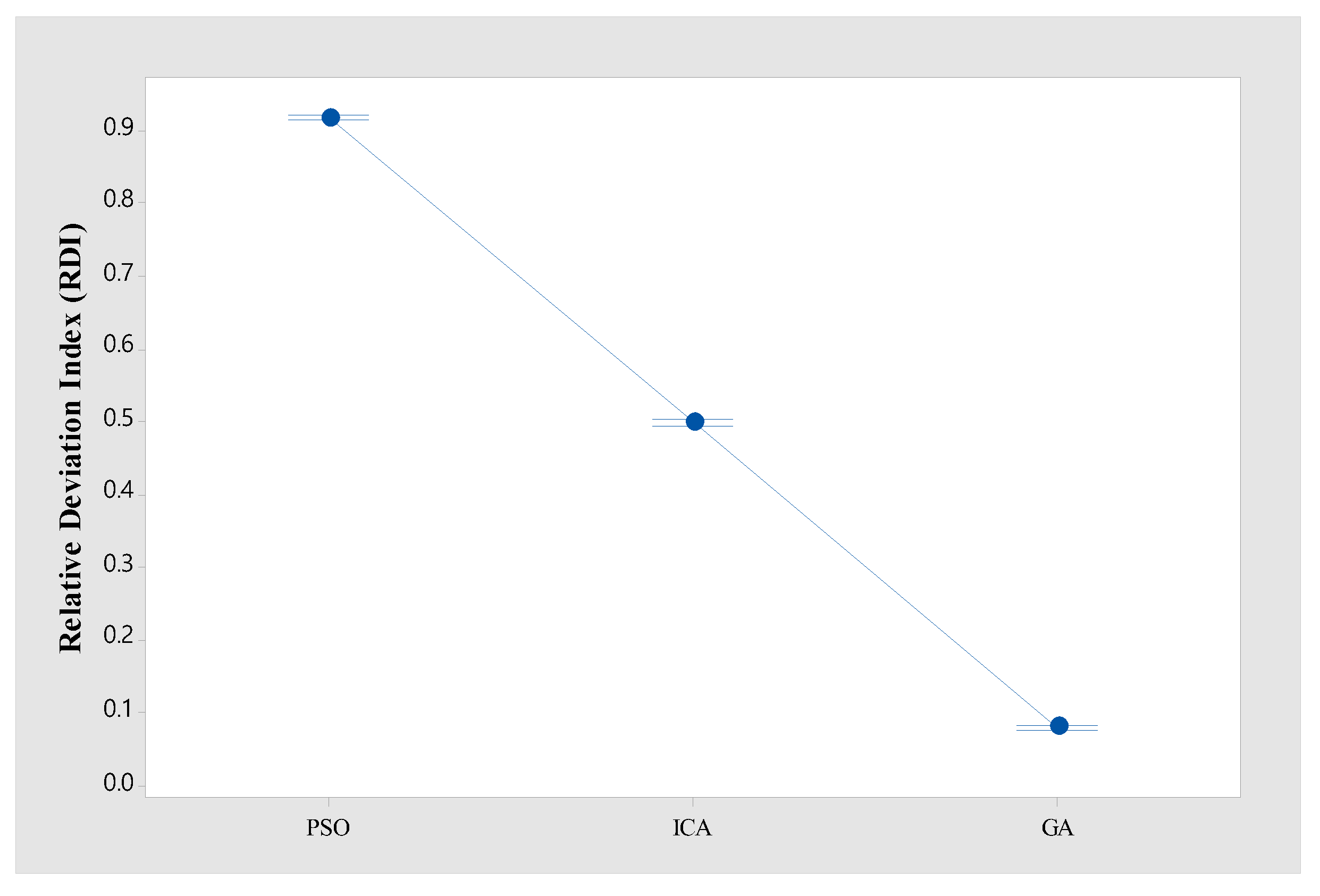
All the algorithms are tested with 30 replications for each instance. Table 7 shows the performance of GA, ICA, and PSO for instances. At δ = 0.6 , the sample means of RDIs for PSO, ICA, and GA for each instance are 0.91, 0.42, and 0.08, respectively. The sample means of CPU times for PSO, ICA, and GA for each instance are 95.10, 56.42, and 95.54, respectively. At δ = 0.3 , the sample means of RDIs for PSO, ICA, and GA are 0.93, 0.58, and 0.08, respectively. The sample means of CPU times for PSO, ICA, and GA are 95.62, 56.50, and 95.70, respectively. The ranking of meta-heuristic algorithms from the best to the worst performance is GA, ICA, and PSO. PSO and GA with the same population size show similar CPU time, and ICA with a relatively smaller population size than PSO and GA shows less CPU time. We execute an additional experiment for ICA with extended CPU time. However, no significant improvement in the RDI of ICA is shown. Therefore, GA shows the best RDI among PSO, ICA, and GA under similar CPU time in large problem instances.
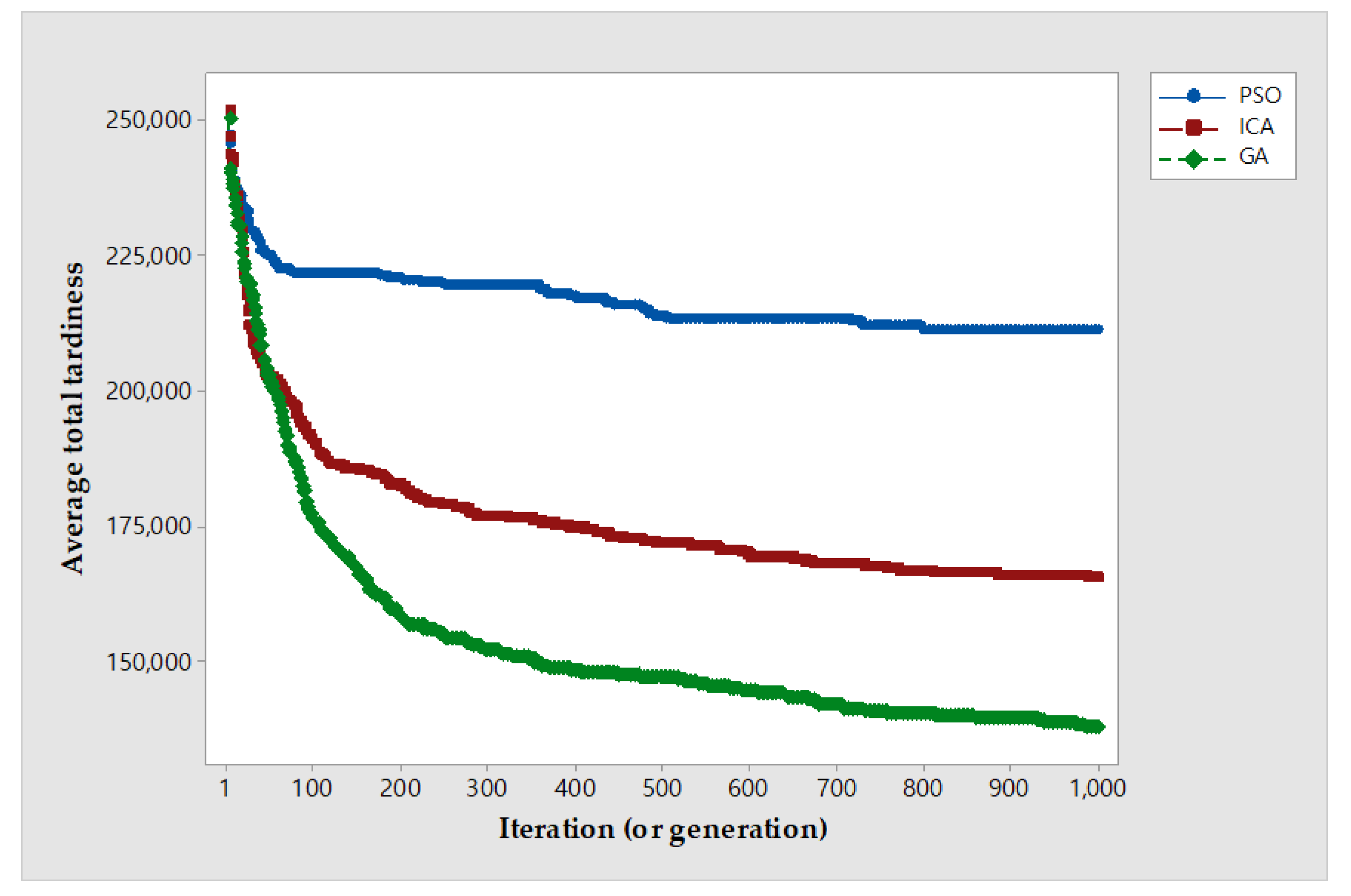
For analysis reasons regarding the performance differences for PSO, ICA, and GA, a convergence test is performed. An instance with | J | = 300 , | T | = 20 , | C | = 20 is used for the test and repeated 10 times. Figure 5 shows the convergence graph for PSO, ICA, and GA. The objective function values of the initial solution are similar for all three algorithms, but PSO and ICA converge faster to a value with a higher objective function than GA. Therefore, GA shows better performance in terms of objective function than PSO and ICA.
To verify the significant difference in RDI between algorithms, the Tukey HSD test was performed. Figure 6 shows the mean plots and Tukey HSD intervals ( α = 0.05 ) for all instances in Table 7. Figure 6 shows that the confidence intervals between all the algorithms do not overlap. In the other words, the difference in RDI between PSO, ICA, and GA is statistically significant.
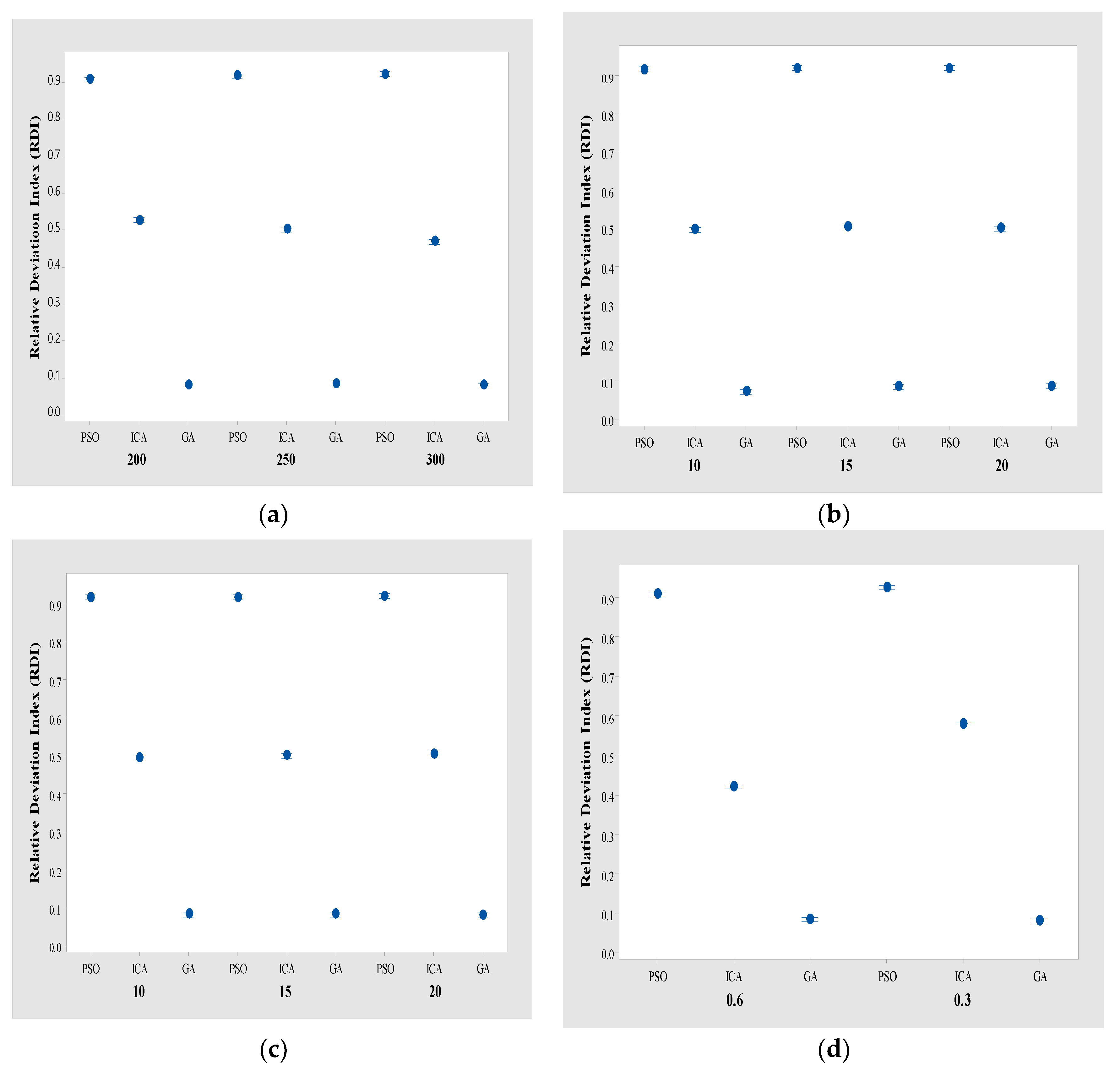
Figure 7 shows the mean plots and Tukey HSD intervals ( α = 0.05 ) for | J | , | T | , | C | , and δ groups. For | J | , | T | , | C | , and δ groups, the performance is ranked in the order of GA, ICA, and PSO, and the difference in RDI between PSO, ICA, and GA is statistically significant. In particular, GA provides the best RDI and robustness among all algorithms.

6. Sensitivity Analysis

To reduce total tardiness for the ISP, scheduling problems of the manufacturing and delivery process are important. It is difficult to find whether manufacturing or delivery scheduling impacts the proposed total tardiness. To find this impact, the total manufacturing completion time ( t M ) and the total delivery time ( t T ) are presented as a performance measure. t M and t T are defined as follows:
t M = j = 1 | J |   c j
t T = j = 1 | J |   ( L e a d j c j )
where c j and L e a d j are the manufacturing completion time and lead time of job j, respectively.
Several problem parameters affect the scheduling of ISPs. Each problem parameter related to the manufacturing and delivery process affects t M and t T , respectively. For example, obviously, t M decreases when V M increases, or p f decreases and t T decreases when | T | or V T increases or h c decreases. However, the effects of parameters related to the manufacturing process on t T and the effects of parameters related to the delivery process on t M are not obvious. To find these effects, an additional experiment is conducted by only using GA with the best performance shown.
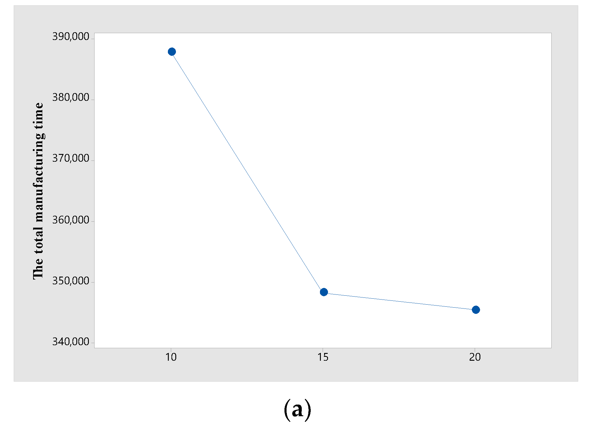
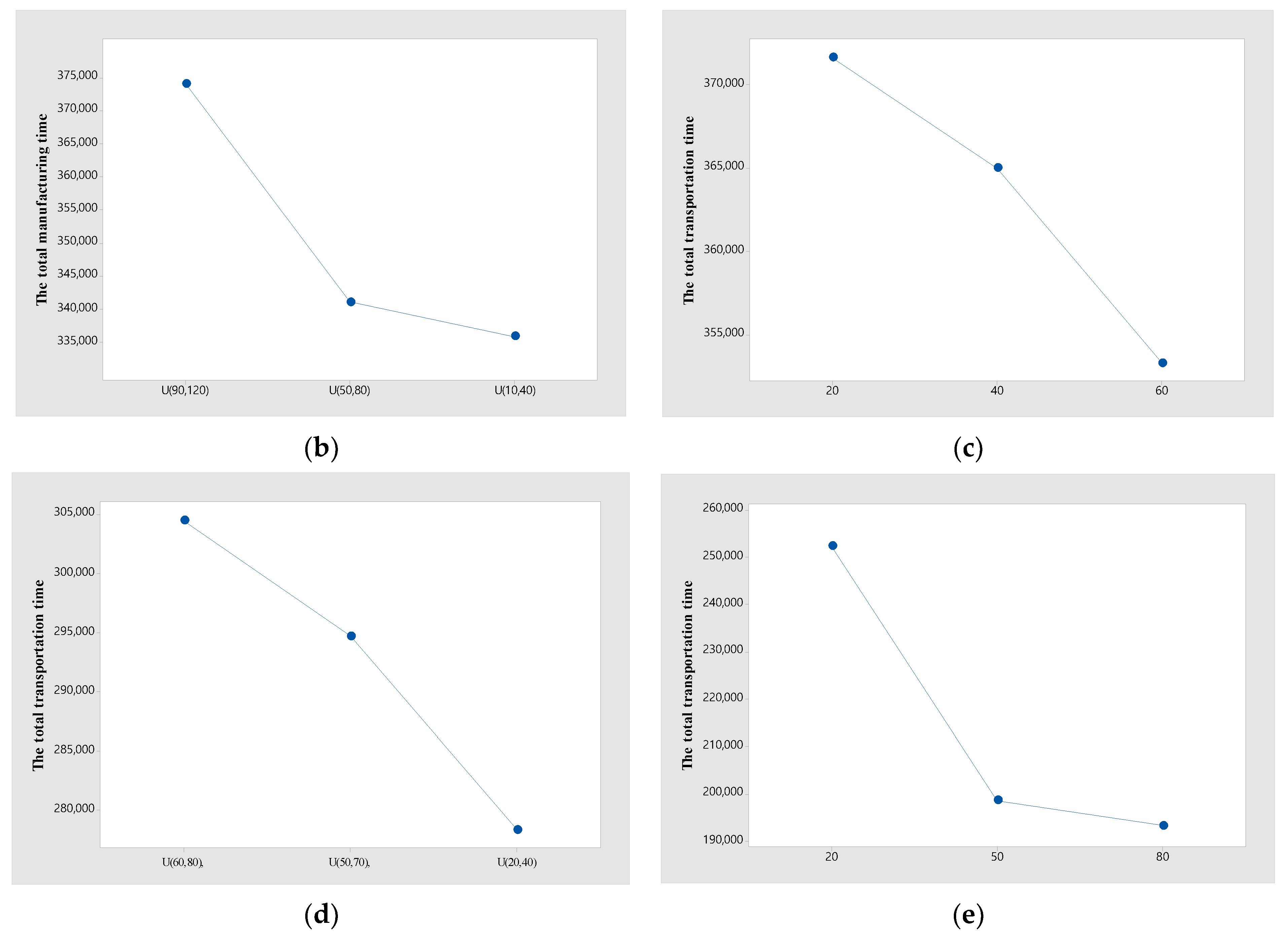
Graphs (a), (b), and (c) in Figure 8 show the change in t M according to the change in the parameters | T | , V T , and h c , respectively. In graphs (a), (b), and (c), t M decreases when | T | or V T increases or h c decreases. Meanwhile, the graphs (d) and (e) in Figure 8 show the change in t T according to the change in the parameters p f and V M . According to the graphs (d) and (e),   t t decreases when V M increases or p f decreases. In summary, the parameters related to the delivery affect t M , and the parameters related to manufacturing affect t T . This is because if the time on one side decreases, the flexibility of decision making on the other side increases. One of the reasons is that the difference in manufacturing completion time between jobs decreases and various decisions in the delivery process become possible as p f decreases.

7. Conclusions

In this research, the ISP with a batching machine, time-dependent batch deterioration, and RMAs is considered. A MILP model was formulated to solve small problem instances. Meta-heuristic algorithms were proposed to solve the large problem instances. The solution structure of meta-heuristics consists of two one-dimensional arrays for manufacturing and delivery. For small problem instances, we found the optimal solution using the developed MILP model. Additionally, we verified the performance of meta-heuristic algorithms by showing the near-optimal solution and comparing it with the MILP model in small problem instances. Three meta-heuristic algorithms, GA, ICA, and PSO, are proposed and relatively compared by using the relative deviation index (RDI) in large problem instances. The ranking of meta-heuristic algorithms from the best to the worst performance was GA, ICA, and PSO. Sensitivity analysis was conducted for GA with the best performance shown. We found that as the time for either manufacturing or delivery was reduced, the time for the other also decreased in this analysis.
However, this study has several limitations. For example, the real enterprise data considered for solving real industry problems are not used, and the objective function is simply set to total tardiness. The objective function can be modeled as a cost including setup, inventory, and tardiness costs. As for further work to extend this study, the problem could apply VRP to our delivery method. In addition, the problem can be extended to optimization problems resolving the conflict of stakeholders between manufacturing and third-party logistics (3PL). Finally, matheuristic and simheuristic approaches can be considered.

Author Contributions

Conceptualization, B.-S.K.; methodology, Y.-J.K.; software, Y.-J.K.; validation, B.-S.K.; formal analysis, Y.-J.K.; investigation, B.-S.K. and Y.-J.K.; resources, B.-S.K.; data curation, Y.-J.K.; writing—original draft preparation, Y.-J.K.; writing—review and editing, B.-S.K.; visualization, Y.-J.K.; supervision, B.-S.K. All authors have read and agreed to the published version of the manuscript.

Funding

This work was supported by the Incheon National University Research Grant in 2021.

Data Availability Statement

Not applicable.

Conflicts of Interest

The authors declare no conflict of interest.

References

  1. Joo, C.M.; Kim, B.S. Rule-based meta-heuristics for integrated scheduling of unrelated parallel machines, batches, and heterogeneous delivery trucks. Appl. Soft Comput. J. 2017, 53, 457–476. [Google Scholar] [CrossRef]
  2. Jia, Z.; Huo, S.; Li, K.; Chen, H. Integrated scheduling on parallel batch processing machines with non-identical capacities. Eng. Optim. 2019, 52, 715–730. [Google Scholar] [CrossRef]
  3. Dobson, G.; Nambimadom, R.S. The Batch Loading and Scheduling Problem. Oper. Res. 2001, 49, 52–65. [Google Scholar] [CrossRef] [Green Version]
  4. Joo, C.M.; Kim, B.S. Variable Neighborhood Search Algorithms for an Integrated Manufacturing and Batch Delivery Scheduling Minimizing Total Tardiness. Appl. Sci. 2019, 9, 4702. [Google Scholar] [CrossRef] [Green Version]
  5. Lee, C.-Y.; Leon, V.J. Machine scheduling with a rate-modifying activity. Eur. J. Oper. Res. 2001, 128, 119–128. [Google Scholar] [CrossRef]
  6. Liu, C.H. Using genetic algorithms for the coordinated scheduling problem of a batching machine and two-stage transportation. Appl. Math. Comput. 2011, 217, 10095–10104. [Google Scholar] [CrossRef]
  7. Selvarajah, E.; Steiner, G. Batch scheduling in a two-level supply chain-a focus on the supplier. Eur. J. Oper. Res. 2006, 173, 226–240. [Google Scholar] [CrossRef]
  8. Gao, S.; Qi, L.; Lei, L. Integrated batch production and distribution scheduling with limited vehicle capacity. Int. J. Prod. Econ. 2015, 160, 13–25. [Google Scholar] [CrossRef]
  9. Cheng, B.-Y.; Leung, J.Y.-T.; Li, K.; Yang, S.-L. Single batch machine scheduling with deliveries. Nav. Res. Logist. 2015, 62, 470–482. [Google Scholar] [CrossRef]
  10. Cheng, B.Y.; Leung, J.Y.T.; Li, K. Integrated scheduling on a batch machine to minimize production, inventory and distribution costs. Eur. J. Oper. Res. 2017, 258, 104–112. [Google Scholar] [CrossRef]
  11. Jia, Z.; Zhuo, X.; Leung, J.Y.T.; Li, K. Integrated production and transportation on parallel batch machines to minimize total weighted delivery time. Comput. Oper. Res. 2019, 102, 39–51. [Google Scholar] [CrossRef]
  12. Li, S.; Yuan, J.; Fan, B. Unbounded parallel-batch scheduling with family jobs and delivery coordination. Inf. Process. Lett. 2011, 111, 575–582. [Google Scholar] [CrossRef]
  13. Li, K.; Jia, Z.H.; Leung, J.Y.T. Integrated production and delivery on parallel batching machines. Eur. J. Oper. Res. 2015, 247, 755–763. [Google Scholar] [CrossRef]
  14. Zhang, J.; Wang, X.; Huang, K. On-line scheduling of order picking and delivery with multiple zones and limited vehicle capacity. Omega 2018, 79, 104–115. [Google Scholar] [CrossRef]
  15. Nogueira, T.H.; Bettoni, A.B.; de Oliveira Mendes, G.T.; dos Santos, A.G.; Ravetti, M.G. Problem on the integration between production and delivery with parallel batching machines of generic job sizes and processing times. Comput. Ind. Eng. 2020, 146, 106573. [Google Scholar] [CrossRef]
  16. Feng, X.; Xu, Z. Integrated Production and Transportation Scheduling on Parallel Batch-Processing Machines. IEEE Access 2019, 7, 148393–148400. [Google Scholar] [CrossRef]
  17. Jia, Z.; Cui, Y.; Li, K. An ant colony-based algorithm for integrated scheduling on batch machines with non-identical capacities. Appl. Intell. 2022, 52, 1752–1769. [Google Scholar] [CrossRef]
  18. He, P.; Li, K.; Kumar, P.N.R. An enhanced branch-and-price algorithm for the integrated production and transportation scheduling problem. Int. J. Prod. Res. 2021, 60, 1874–1889. [Google Scholar] [CrossRef]
  19. Li, K.; He, P.; Ram Kumar, P.N. A column generation based approach for an integrated production and transportation scheduling problem with dual delivery modes. Int. J. Prod. Res. 2022. [CrossRef]
  20. Karaoğlan, İ.; Kesen, S.E. The coordinated production and transportation scheduling problem with a time-sensitive product: A branch-and-cut algorithm. Int. J. Prod. Res. 2017, 55, 536–557. [Google Scholar] [CrossRef]
  21. Low, C.; Chang, C.M.; Li, R.K.; Huang, C.L. Coordination of production scheduling and delivery problems with heterogeneous fleet. Int. J. Prod. Econ. 2014, 153, 139–148. [Google Scholar] [CrossRef]
  22. Low, C.; Chang, C.M.; Gao, B.Y. Integration of production scheduling and delivery in two echelon supply chain. Int. J. Syst. Sci. Oper. Logist. 2017, 4, 122–134. [Google Scholar] [CrossRef]
  23. Li, K.; Zhou, C.; Leung, J.Y.T.; Ma, Y. Integrated production and delivery with single machine and multiple vehicles. Expert Syst. Appl. 2016, 57, 12–20. [Google Scholar] [CrossRef]
  24. Kong, L.; Li, H.; Luo, H.; Lieyun, D.; Luo, X.; Skitmore, M. Optimal single-machine batch scheduling for the manufacture, transportation and JIT assembly of precast construction with changeover costs within due dates. Autom. Constr. 2017, 81, 34–43. [Google Scholar] [CrossRef] [Green Version]
  25. Liu, X.; Lu, S.; Pei, J.; Pardalos, P.M. A hybrid VNS-HS algorithm for a supply chain scheduling problem with deteriorating jobs. Int. J. Prod. Res. 2018, 56, 5758–5775. [Google Scholar] [CrossRef]
  26. Yin, Y.; Cheng, T.C.E.; Wu, C.C.; Cheng, S.R. Single-machine batch delivery scheduling and common due-date assignment with a rate-modifying activity. Int. J. Prod. Res. 2014, 52, 5583–5596. [Google Scholar] [CrossRef]
  27. Joo, C.M.; Kim, B.S. Genetic algorithms for single machine scheduling with time-dependent deterioration and rate-modifying activities. Expert Syst. Appl. 2013, 40, 3036–3043. [Google Scholar] [CrossRef]
  28. Vélez-Gallego, M.C.; Damodaran, P.; Rodríguez, M. Makespan minimization on a single batch processing machine with unequal job ready times. Int. J. Ind. Eng. Theory Appl. Pract. 2011, 18, 536–546. [Google Scholar]
  29. Wang, H.M.; Chou, F. Der Solving the parallel batch-processing machines with different release times, job sizes, and capacity limits by metaheuristics. Expert Syst. Appl. 2010, 37, 1510–1521. [Google Scholar] [CrossRef]
  30. Marandi, F.; Fatemi Ghomi, S.M.T. Integrated multi-factory production and distribution scheduling applying vehicle routing approach. Int. J. Prod. Res. 2019, 57, 722–748. [Google Scholar] [CrossRef]
  31. Bean, J.C. Genetic Algorithms and Random Keys for Sequencing and Optimization. Inf. J. Comput. 1994, 6, 154–160. [Google Scholar] [CrossRef]
  32. Mosadegh, H.; Zandieh, M.; Ghomi, S.M.T.F. Simultaneous solving of balancing and sequencing problems with station-dependent assembly times for mixed-model assembly lines. Appl. Soft Comput. J. 2012, 12, 1359–1370. [Google Scholar] [CrossRef]
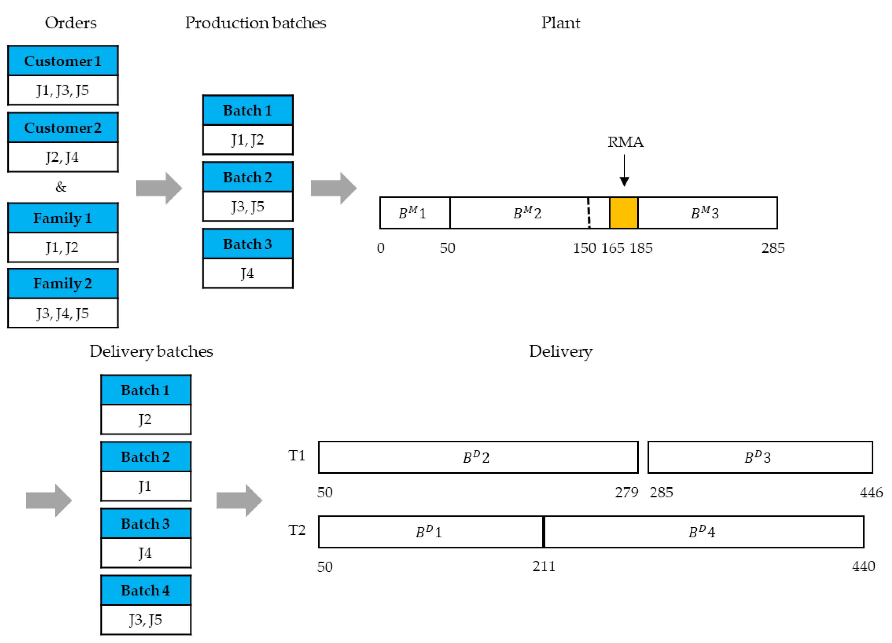
Figure 1. A Gantt chart example of schedules for the presented ISP.
Mathematics 10 04127 g001
Figure 2. An example of decoding procedure for manufacturing.
Mathematics 10 04127 g002
Figure 3. An example of decoding procedure for delivery.
Mathematics 10 04127 g003
Figure 4. The mean S/N ratio and RDI plot for each GA parameter. (a) S/N ratio, (b) RDI.
Mathematics 10 04127 g004
Figure 5. The convergence graph for PSO, ICA, and GA.
Mathematics 10 04127 g005
Figure 6. The mean plots and Tukey HSD intervals ( α = 0.05 ) for PSO, ICA, and GA.
Mathematics 10 04127 g006
Figure 7. The mean plots and Tukey HSD intervals ( α = 0.05 ) for | J | , | T | , | C | , and δ groups. (a) | J | group. (b) | T | group. (c) | C | group. (d) δ group.
Mathematics 10 04127 g007
Figure 8. Total manufacturing and delivery time under different | T | , h c , V T ,   p f , and   V M . (a) Total manufacturing time under different | T | . (b) Total manufacturing time under different h c . (c) Total manufacturing time under different V T . (d) Total delivery time under different p f . (e) Total delivery time under different V M .
Mathematics 10 04127 g008aMathematics 10 04127 g008b
Table 1. Classification for Studies on ISP with batch processing.
Compatibility in Production BatchesVehicles NumberDeteriorationRMAShipping Method
Incompatible ProductIncompatible FamilyIncompatible CustomerDirect-ShippingVRP
Liu [6] 1
Jia et al. [2] Limited
Selvarajah and Steiner [7] 1
Gao et al. [8] 1
Cheng et al. [9] 1
Cheng et al. [10] 1
Jia et al. [11] Limited
Li et al. [12] 1
Li et al. [13] Limited
Zhang et al. [14] 1
Nogueira et al. [15] Limited
Feng and Xu [16] Unlimited
Jia et al. [17] Limited
He et al. [18] Limited
Li et al. [19] Limited
Karaoğlan and Kesen [20] 1
Low et al. [21] Unlimited
Low et al. [22] Limited
Li et al. [23] Limited
Kong et al. [24] Unlimited
Liu et al. [25] 1
Yin et al. [26] Unlimited
This study Limited
Table 2. The value of each level of GA parameters.
ParametersLevels
12345
G s 2004006008001000
P s 20406080100
p c 0.10.30.50.70.9
p m 0.0010.0020.0030.0040.004
Table 3. Orthogonal arrays for GA parameters.
Run G s P s p c p m
1 G s ( 1 ) P s ( 1 ) p c ( 1 ) p m ( 1 )
2 G s ( 1 ) P s ( 2 ) p c ( 2 ) p m ( 2 )
3 G s ( 1 ) P s ( 3 ) p c ( 3 ) p m ( 3 )
4 G s ( 1 ) P s ( 4 ) p c ( 4 ) p m ( 4 )
5 G s ( 1 ) P s ( 5 ) p c ( 5 ) p m ( 5 )
6 G s ( 2 ) P s ( 1 ) p c ( 2 ) p m ( 3 )
7 G s ( 2 ) P s ( 2 ) p c ( 3 ) p m ( 4 )
8 G s ( 2 ) P s ( 3 ) p c ( 4 ) p m ( 5 )
9 G s ( 2 ) P s ( 4 ) p c ( 5 ) p m ( 1 )
10 G s ( 2 ) P s ( 5 ) p c ( 1 ) p m ( 2 )
11 G s ( 3 ) P s ( 1 ) p c ( 3 ) p m ( 5 )
12 G s ( 3 ) P s ( 2 ) p c ( 4 ) p m ( 1 )
13 G s ( 3 ) P s ( 3 ) p c ( 5 ) p m ( 2 )
14 G s ( 3 ) P s ( 4 ) p c ( 1 ) p m ( 3 )
15 G s ( 3 ) P s ( 5 ) p c ( 2 ) p m ( 4 )
16 G s ( 4 ) P s ( 1 ) p c ( 4 ) p m ( 2 )
17 G s ( 4 ) P s ( 2 ) p c ( 5 ) p m ( 3 )
18 G s ( 4 ) P s ( 3 ) p c ( 1 ) p m ( 4 )
19 G s ( 4 ) P s ( 4 ) p c ( 2 ) p m ( 5 )
20 G s ( 4 ) P s ( 5 ) p c ( 3 ) p m ( 1 )
21 G s ( 5 ) P s ( 1 ) p c ( 5 ) p m ( 4 )
22 G s ( 5 ) P s ( 2 ) p c ( 1 ) p m ( 5 )
23 G s ( 5 ) P s ( 3 ) p c ( 2 ) p m ( 1 )
24 G s ( 5 ) P s ( 4 ) p c ( 3 ) p m ( 2 )
25 G s ( 5 ) P s ( 5 ) p c ( 4 ) p m ( 3 )
Table 4. ANOVA result for S/N ratio of GA parameters.
ParametersSSdfV F 0 p-Value
G s 4.098341.02463.62190.1202
P s 5.119041.27974.52390.0865
p c 2.385340.59632.10800.2439
p m (error) 1.131540.2829--
Total12.734216---
Table 5. Problem parameter setting.
GroupPH | J | p f h c v j V M V T D R Q d j
τ = 0.6 τ = 0.3
Small problem instances4805[65,100][130,200][5,10]20200.3165[48,336]NA
6[55,90][110,180][5,10]20200.3145
Large problem instances2400200[30,45][60,90][5,10]50200.375[240,1680][420,2940]
250[25,35][50,70][5,10]50200.360
300[20,30][40,60][5,10]50200.350
Table 6. Computational results for small problem instances ( τ = 0.6 ).
| J | | T | | C | | F | CPLEXPSOICAGA
O p t . Time O b j s o l Time O b j s o l Time O b j s o l Time
5111584.001.05584.00 0.26 584.00 0.11584.00 0.27
2844.002.03844.00 0.26 844.83 0.11846.66 0.28
21484.000.77484.00 0.25 484.00 0.11484.00 0.27
2980.000.34980.00 0.25 980.00 0.11980.00 0.28
211675.804.57675.80 0.24 675.80 0.11675.80 0.26
2949.4025.03949.40 0.24 949.40 0.11949.40 0.26
21365.0027.30365.00 0.26 365.00 0.11365.00 0.28
2437.0011.60437.00 0.25 437.00 0.11437.00 0.28
6111633.004.13633.00 0.31 639.72 0.14633.00 0.33
2770.0011.83770.000.31771.470.14770.000.33
21629.001.62629.000.32629.430.14629.000.34
2821.002.67821.00 0.30 821.00 0.13821.00 0.32
211NA7200.00++1031.33 0.32 1031.33 0.141031.33 0.33
2671.03104.65671.030.31671.030.14671.030.34
21NA7200.00++886.98 0.35 887.83 0.14886.98 0.34
2NA7200.00++608.70 0.35 618.07 0.15599.32 0.36
Average 710.640.29711.870.13710.220.30
Table 7. Computational results for large problem instances.
| J | | T | | C | τ = 0.6 τ = 0.3
PSOICAGAPSOICAGA
RDITimeRDITimeRDITimeRDITimeRDITimeRDITime
20010100.90 61.01 0.43 35.95 0.09 61.41 0.90 61.44 0.60 36.22 0.08 61.52
150.91 61.32 0.43 36.30 0.06 61.30 0.91 61.78 0.56 36.19 0.07 61.63
200.89 61.58 0.44 36.37 0.05 61.88 0.93 61.87 0.60 36.15 0.06 61.87
15100.89 61.66 0.46 36.51 0.12 62.42 0.92 62.08 0.58 36.75 0.07 62.57
150.90 62.15 0.41 37.11 0.07 62.59 0.93 62.44 0.61 36.95 0.06 62.66
200.87 62.23 0.46 37.01 0.08 62.36 0.91 62.60 0.65 36.97 0.08 63.47
20100.90 62.35 0.45 36.84 0.07 62.79 0.92 62.48 0.58 36.94 0.08 62.55
150.93 62.59 0.44 37.01 0.11 63.25 0.93 63.07 0.65 37.06 0.08 62.69
200.91 62.91 0.50 37.28 0.10 63.29 0.93 63.05 0.64 37.24 0.11 62.78
25010100.92 92.04 0.48 54.58 0.09 92.22 0.92 92.22 0.56 54.31 0.09 91.90
150.91 92.29 0.46 54.80 0.05 92.04 0.91 92.84 0.59 54.65 0.08 92.39
200.93 92.56 0.44 54.71 0.06 92.71 0.94 93.15 0.54 54.82 0.09 92.60
15100.92 92.71 0.38 55.46 0.10 93.34 0.95 93.12 0.59 55.23 0.09 93.55
150.89 92.86 0.43 54.99 0.08 93.40 0.92 93.69 0.61 55.57 0.11 93.55
200.93 94.02 0.42 55.56 0.10 93.64 0.94 94.12 0.62 55.64 0.10 93.10
20100.88 92.97 0.39 55.52 0.11 93.88 0.91 93.72 0.55 55.59 0.04 93.50
150.93 93.95 0.43 56.12 0.11 94.18 0.93 94.67 0.57 56.05 0.09 94.78
200.88 94.15 0.42 56.08 0.05 94.42 0.93 94.51 0.58 56.00 0.07 94.28
30010100.92 128.67 0.42 76.30 0.07 129.12 0.94 129.57 0.54 76.79 0.07 129.18
150.90 129.55 0.44 76.98 0.06 129.14 0.89 130.33 0.47 76.68 0.05 130.27
200.94 130.14 0.39 77.45 0.10 130.51 0.93 130.49 0.53 76.80 0.07 130.07
15100.91 129.47 0.39 77.02 0.08 129.98 0.94 130.03 0.58 77.43 0.07 130.23
150.95 130.62 0.37 78.09 0.10 132.10 0.93 131.17 0.59 77.20 0.08 130.83
200.92 130.78 0.38 78.12 0.06 131.46 0.93 131.81 0.55 77.85 0.08 131.70
20100.92 130.49 0.39 77.74 0.08 131.14 0.95 131.34 0.54 78.01 0.07 132.78
150.91 131.13 0.35 78.68 0.09 132.44 0.93 131.89 0.57 77.93 0.11 133.99
200.92 131.58 0.36 78.08 0.10 132.49 0.94 132.35 0.58 78.51 0.08 133.41
Average0.9195.100.4256.420.0895.540.9395.620.5856.500.0895.70
Publisher’s Note: MDPI stays neutral with regard to jurisdictional claims in published maps and institutional affiliations.