Abstract
Breast cancer (BC) is one of the deadly forms of cancer, causing mortality worldwide in the female population. The standard imaging procedures for screening BC involve mammography and ultrasonography. However, these imaging procedures cannot differentiate subtypes of benign and malignant cancers. Here, histopathology images could provide better sensitivity toward benign and malignant cancer subtypes. Recently, vision transformers have been gaining attention in medical imaging due to their success in various computer vision tasks. Swin transformer (SwinT) is a variant of vision transformer that works on the concept of non-overlapping shifted windows and is a proven method for various vision detection tasks. Thus, in this study, we investigated the ability of an ensemble of SwinTs in the two-class classification of benign vs. malignant and eight-class classification of four benign and four malignant subtypes, using an openly available BreaKHis dataset containing 7909 histopathology images acquired at different zoom factors of 40×, 100×, 200×, and 400×. The ensemble of SwinTs (including tiny, small, base, and large) demonstrated an average test accuracy of 96.0% for the eight-class and 99.6% for the two-class classification, outperforming all the previous works. Thus, an ensemble of SwinTs could identify BC subtypes using histopathological images and may lead to pathologist relief.
MSC:
68T45
1. Introduction
Breast cancer (BC) is the second deadliest cancer after lung cancer, causing morbidity and mortality worldwide in the female population [1]. Its incidence may increase by more than 50% by the year 2030 in the United States [2]. The non-invasive diagnostic procedures for BC involve physical examination and imaging techniques such as mammography, ultrasonography, and magnetic resonance imaging [3,4]. However, physical examination may not detect it early, and imaging procedures offer low sensitivity for a more comprehensive assessment of cancerous regions and identification of cancer subtypes [5,6]. Histopathological imaging via breast biopsy, even though minimally invasive, may provide accurate identification of the cancer subtype and precise localization of the lesion [7]. However, this manual examination by the pathologist could be tiresome and prone to errors. Therefore, automated methods for BC subtype classification are warranted. Deep learning has revolutionized many areas in the last decade, including healthcare, for various tasks such as accurate disease diagnosis and prognosis and robotic-assisted surgery [8]. There were studies based on deep convolutional neural networks (CNN) for detecting BC using the aforementioned imaging procedures [9]. However, CNNs exhibit inherent inductive bias and are variant to translation, rotation, and location of the object of interest in the image. Therefore, image augmentation is generally applied while training CNN models, although the data augmentation may not provide expected variations in the training set. Thus, self-attention-based deep learning models that are more robust towards the orientation and location of an object of interest in the image are rapidly growing [10].
In recent years, encoder-decoder-based transformers have become the de facto models in natural language processing. Vision transformer (ViT), the adaptation of transformers to deal with images, proved to be an excellent alternative to CNNs under high-data regimes [11]. However, the ViT for classification tasks implements global self-attention, where associations between an image patch and all other patches are computed. This global quantification leads to quadratic computational complexity concerning the number of patches, making it less suitable for handling high-resolution images. Recently, a variant of ViT called the swin transformer (SwinT) has been proposed that works on shifted windows and provides variable image patch resolutions.
SwinTs are an improved version of ViT architecture and are hierarchical vision transformers using shifted windows [12]. For efficient modeling, self-attention within local windows was proposed and computed, and in order to evenly partition the image, the windows are arranged in a non-overlapping manner. The window-based self-attention has linear complexity and is scalable. However, the modeling power of window-based self-attention is limited, because it lacks connections across windows. Therefore, a shifted window partitioning approach that alternates between the partitioning configurations in consecutive swin transformer blocks was proposed to allow cross-window connections while maintaining the efficient computation of non-overlapping windows. The shifted window scheme in swin transformers offers increased efficiency by restricting self-attention computation to local windows that are non-overlapping while also facilitating a cross-window connection. Overall, the SwinT network’s performance was superior to that of the standard ViTs [12].
To our knowledge, no study exists for automated multi-class classification of BC from histopathology images using SwinT models. Therefore, the main contributions of this study are listed below.
- i.
- We investigated the ability of existing SwinT models for both binary (benign vs. malignant) and eight-class (includes four benign and four malignant subtypes) classification without disturbing their architectures to enable effective transfer learning.
- ii.
- Further, we investigated the power of ensemble learning, and the results indicated that the ensemble of these four SwinT models (BreaST-Net) indeed provided better performance relative to individual models’ performance for both binary as well as multi-class classification tasks.
- iii.
- Furthermore, for the multi-class classification, the models ensembling was implemented using the dataset as a whole and using the dataset stratified with respect to the images acquired at zoom factors 50×, 100×, 200×, and 400×.
- iv.
- Eventually, the five-fold cross-validation and testing were implemented for all of the individual as well as the ensemble models.
2. Related Work
2.1. Based on Mammography
In the literature, there have been many studies related to the diagnosis of BC from mammograms based on traditional machine learning (ML) and neural network-based deep learning (DL) methods [13,14,15]. The typical features to consider from the mammogram during classification from a specific region of interest (ROI) were mass size, regular/irregular shape of ROIs, homogeneity of ROI boundaries, and density of the tissues. These handcrafted features were fed to several classifiers, such as support vector machines, k-nearest neighbor, logistic regression, binary decision tree, and artificial neural network, to classify the mammogram into healthy or cancerous (benign or malignant) [16]. However, the performance of these classifiers depends on other intermediate steps, such as image enhancement and tumor region segmentation. Further, several DL-based methods from the transfer learning of AlexNet, GoogLeNet, ResNet50, multistage fine-tuned CNN, generative adversarial network, autoencoder, and multi-ResNet were implemented for the breast mass classification [16]. DL-based methods generally offer better sensitivity for BC classification than ML-based techniques.
2.2. Based on Ultrasonography
Ultrasonography is also non-invasive and more portable and more sensitive to the disease than mammography [17,18]. There exist both ML- and DL-based methods for the classification of BC from ultrasound images. The ML-based methods include ROI-based radiomic features for classification using various ML classifiers. The Hilbert transform and marker-controlled watershed transform were used to extract shape and textural features that were further fed to a kNN classifier and ensemble decision tree model [19]. The DL-based methods majorly involve fine-tuning the existing CNN models. In [20], semantic segmentation, fuzzy logic, and eight pre-trained CNN models were used for BC classification. In another study [21], deep representation scaling layers between pre-trained CNN blocks were employed for better information flow, and the resulting model demonstrated improved performance. Several other studies include shape adaptive CNN, U-Net encoder-decoder CNN architecture, dilated semantic segmentation technique, and reformed features from DarkNet53 [22]. Overall, BC classification from ultrasound images has been well studied, and most of the studies were based on the familiar BUSI dataset [22].
2.3. Based on Histopathology
The non-invasive imaging procedures described above may be incapable of identifying cancer areas and their subtypes. To compensate for this shortcoming, a biopsy is used to more diversely study malignancy in breast tissues. A biopsy involves collecting the samples and staining the tissue mounted on the microscopic glass slides to visualize cytoplasm and nuclei better [23]. In a recent study, an ensemble of fine-tuned VGG16 and VGG19 CNN models was implemented for a two-class classification of carcinoma vs. non-carcinoma from 544 whole slide images [24]. In other recent studies [25,26] using the BreaKHis dataset, a modified residual neural network and an image moments-based artificial neural network, respectively, were implemented for benign vs. malignant classification using the images at 40× zoom factor alone. A stain acclimation generative adversarial network was developed lately and tested on various publicly available datasets for binary and four-class classification tasks [27]. In another recent study using the BreaKHis dataset, four-class and eight-class classification schemes were developed using a novel deep 6B-Net [28]. CNNs usually exhibit strong inductive bias that they are sensitive to local pixel variations in the image. However, transformer architecture-inspired models for the image data, such as ViT and SwinTs, exhibit less inductive bias due to the embedding of patch positional information with patch embeddings. Therefore, to our knowledge, none of the works have been implemented using SwinTs for the two-class and eight-class classifications of BC from histopathology images obtained from breast biopsy.
3. Methods
3.1. Dataset
The BreaKHis dataset consists of 7909 microscopic RGB images via the surgical biopsy of breast tumors from 82 patients acquired at 50×, 100×, 200×, and 400× magnification factors [29]. Figure 1 includes sample images of the dataset at various zoom factors. The data contain both benign and malignant subtypes. Further, the benign cancer subtypes include fibroadenoma, tubular adenoma, phyllodes tumor, and adenosis, whereas the malignant subtypes contain ductal carcinoma, papillary carcinoma, lobular carcinoma, and mucinous carcinoma. Table 1 includes complete details about the dataset stratified for tumor type and magnification factors.
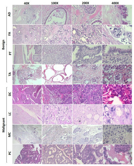
Figure 1.
Sample images from the BreaKHis dataset shown at 40×, 100×, 200×, and 400× magnification factors. AD: adenosis, FA: fibroadenoma, PT: phyllodes tumor, TA: tubular adenoma, DC: ductal carcinoma, LC: lobular carcinoma, MC: mucinous carcinoma, PC: papillary carcinoma.

Table 1.
Number of images at 40×, 100×, 200×, and 400× magnification factors from BreaKHis dataset stratified with respect to cancer subtype. FA: fibroadenoma, TA: tubular adenoma, PT: phyllodes tumor, AD: adenosis, DC: ductal carcinoma, LC: lobular carcinoma, MC: mucinous carcinoma, PC: papillary carcinoma, N: number of images.
3.2. Swin Transformer
An overview of the SwinT model architecture is detailed in Figure 2 below for the base version of SwinT. Firstly, the original image resolution of 700 × 460 is resized to 224 × 224, as it is a requirement for pre-trained and fine-tuned SwinTs. Further, the input RGB image with input dimension H × W × 3 is split into smaller patches of size equal to 4 × 4 following the starting patch size in the original implementation. Thus, the dimension of each image patch is 4 × 4 × 3 = 48. Subsequently, a linear embedding layer is applied on this raw feature tensor of size 48 to project it to an arbitrary feature dimension C. Several swin transformer blocks with modified self-attention are applied on these patch linear embeddings of size C and maintain the number of tokens equal to . The linear embedding layer along with swin transformer blocks constitutes Stage 1 of the swin transformer architecture. To facilitate a hierarchical representation, the number of patches is lowered by patch merging layers starting from Stage 2 of the SwinT-B architecture. The patch merging layer in Stage 2 concatenates the features of each group of 2 × 2 neighboring patches and applies a linear layer on the 4C dimensional concatenated features. This reduces the number of patches by a factor of 4, and the output depth of the linear layer is set to 2C. Further, swin transformer blocks are applied for feature transformation, while the number of output patches of Stage 2 is kept at . This procedure is repeated twice, constituting Stage 3 and Stage 4, leading to an output resolution of and , respectively. These stages jointly produce a deep hierarchical representation with the feature map sizes typical of conventional CNN architectures, such as VGGNets [30] and ResNets [31].
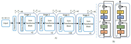
Figure 2.
(A) The architecture for the swin transformer base model. (B) Two successive swin transformer blocks (notations given with Equations (1)–(4)). LN: layer normalization, W-MSA: window (regular) multi-head self-attention, SW-MSA: shifted window multi-head self-attention, MLP: multi-layer perceptron. Input image size is 224 × 224 × 3, C = 128, and layer numbers = .
The models employed were Swin-T (tiny), Swin-S (small), Swin-B (base), and Swin-L (large). Tiny and small models were pre-trained on the ImageNet-1K dataset, whereas base and large models were pre-trained on the ImageNet-22K dataset and fine-tuned on ImageNet-1K dataset, since base and large models have relatively much higher parameters to train. Using the shifted window partitioning procedure, consecutive swin transformer blocks were computed using the mathematical expressions given below in Equations (1)–(4), where and denote the output features of WMSA and the MLP module for block l, respectively. Similarly, and represent outputs of SWMSA and MLP for block l + 1, respectively. In each swin transformer block, layer normalization was applied before multi-head self-attention and MLP.
3.3. Model Cross-Validation and Testing
The intensity values of the images in the original dataset were between 0 and 255. These intensities were rescaled to have values between −1 and 1 using the pre-processing method available in the vit-keras module. The dataset was divided into 62:8:30 for training, validation, and testing, respectively, when images across all zoom factors were included. When the classification was implemented from the images of a specific zoom factor, a 72:8:20 split was followed. The hyperparameters of the swin transformers were chosen empirically, and the validation set was used to make sure that the model was not overfitting. The optimizer included during cross-validation was Adadelta with 0.1 as the learning rate. Other hyperparameters were sparse categorical cross-entropy as the loss function, batch sizes of 32 for tiny and small models, 16 for the base, and 8 for large models, and the number of epochs was equal to 15 for all cases.
3.4. Performance Metrics
Since the number of samples in each tumor type is imbalanced, along with accuracy, other performance metrics, such as the area under the receiver operating characteristics curve (AUC), F1-score, balanced accuracy (BA), Matthew’s correlation coefficient (MCC), and confusion matrices, were employed. The MCC is an excellent choice when there is a class imbalance [32,33]. The mathematical expressions for various performance metrics based on true positives (TP), true negatives (TN), false positives (FP), and false negatives (FN) are given below. For eight-class classification, one vs. rest approach was used for calculating the recall, specificity, and precision. From the confusion matrix, the misclassifications above the off-diagonal were considered as FPs, and the number of misclassifications below the off-diagonal was categorized as FNs. The TNs are number of correctly classified for the other classes than the specific class. The mathematical expressions for the performance metrics are given below in Equations (5)–(10).
3.5. Model Ensembling
An ensemble model was implemented based on averaging the predicted softmaxi vectors of N individual models, mathematically described in Equation (11). The final class prediction is the index of the highest probability in vector that is given in Equation (12).
4. Results
4.1. Two-Class Classification
Although the validation performance scores are uninformed, they are close to test performance metrics in all scenarios. The best individual model for two-class classification was Swin-L, with a test accuracy equal to 99.2%, AUC of 99.1%, F1-score of 99.2%, BA of 99.1%, and MCC of 98.3%. The average ensembling of the four swin transformers yielded an accuracy of 99.5%, AUC of 99.4%, 99.5% F1-score, 99.4% BA, and 98.9% MCC. Complete performance metrics on the test set for the two-class classification by aggregation of images across all magnification factors are given in Table 2. In addition, the confusion matrix on the test set for each model is in Figure 3. For the ensemble model, the prediction accuracies for benign and malignant tumors were 99.0% and 99.8%, respectively.
Table 2.
Performance metric values on the test set for the two-class classification (benign vs. malignant) of BC by considering images from all zoom factors. AUC: area under the receiver operating characteristic curve, BA: balanced accuracy, MCC: Matthew’s correlation coefficient, T: tiny, S: small, B: base, L: large.
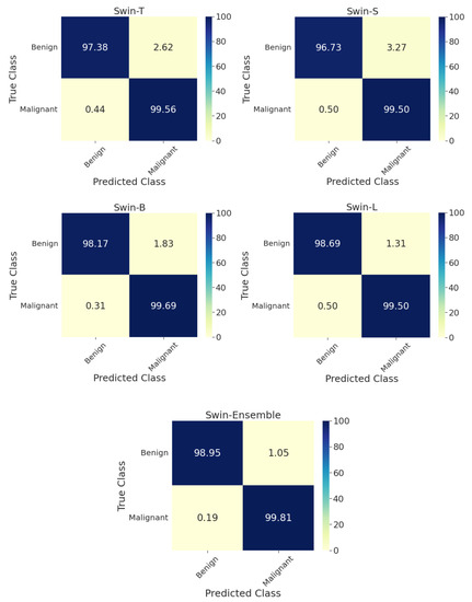
Figure 3.
Confusion matrices on the test set for the two-class classification of benign and malignant types for individual swin transformer model as well as the average ensemble model by considering images from all zoom factors. T: tiny, S: small, B: base, L: large.
4.2. Eight-Class Classification
Since eight-class classification was the prime objective of this study, the ability of the swin transformer models in the classification was investigated for the whole dataset and stratified with respect to the zoom factors as given in Table 3. In all scenarios, the ensemble model performed better than the individual models. The best model at 40× was Swin-L, with a test accuracy of 95.5%, AUC of 99.7%, F1-score of 95.4%, BA of 94.9%, and MCC of 94.1%. However, the average ensembling yielded an accuracy of 96.0%, AUC of 99.7%, 95.8% of F1-score, 95.5% of BA, and MCC of 94.7%. At all other zoom factors, the ensemble model’s performance was best, and Swin-L was the best individual performer. A similar trend was observed by considering the whole dataset.
Table 3.
Performance metric values on the test set for the eight-class classification (subtypes as listed in Table 1) of BC stratified with respect to images acquired at different zoom factors. AUC: area under the receiver operating characteristic curve, BA: balanced accuracy, MCC: Matthew’s correlation coefficient, T: tiny, S: small, B: base, L: large.
Figure 4 shows the confusion matrices for individual and the ensemble models by considering the whole dataset. More than 10 percent of phyllodes tumor images were misclassified as fibroadenoma, and around 25 percent of lobular carcinomas were wrongly classified as ductal carcinoma. All swin models achieved a classification accuracy of 100% for adenosis. Further, the confusion matrices for the ensemble model’s performance on the test set at different zoom factors are in Figure 5. The ensemble model at 40× zoom factor outperformed the ensemble models at the other zoom factors. Furthermore, it demonstrated an accuracy of 100% for the classification of fibroadenoma, tubular adenoma, adenosis, phyllodes carcinoma, and mucinous carcinoma. Most of the misclassifications for the 40× ensemble model happened for lobular carcinoma images that were wrongly classified as ductal carcinoma.
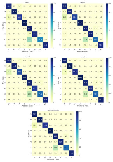
Figure 4.
Confusion matrices on the test set for the eight-class classification of benign and malignant subtypes for each swin transformer model by considering images from all zoom factors. T: tiny, S: small, B: base, L: large. FA: fibroadenoma, TA: tubular adenoma, PT: phyllodes tumor, AD: adenosis, DC: ductal carcinoma, PC: papillary carcinoma, LC: lobular carcinoma, MC: mucinous carcinoma.
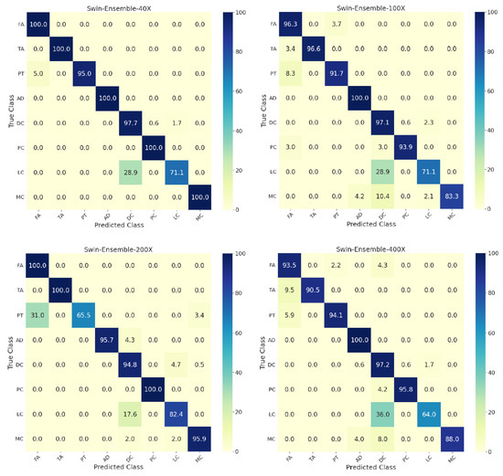
Figure 5.
Confusion matrices on the test set for the eight-class classification of benign and malignant subtypes for the ensemble of swin transformers at 40×, 100×, 200×, and 400× zoom factors. T: tiny, S: small, B: base, L: large. FA: fibroadenoma, TA: tubular adenoma, PT: phyllodes tumor, AD: adenosis, DC: ductal carcinoma, PC: papillary carcinoma, LC: lobular carcinoma, MC: mucinous carcinoma.
5. Discussion
In this study, the effectiveness of the ensemble of SwinTs (BreaST-Net) for automated classification of BC from histopathological images was studied for both two-class (benign tumor vs. malignant tumor) and eight-class (all subtypes) classification regimes using the BreaKHis dataset. For the two-class classification, the ensemble model demonstrated an accuracy of 99.6%, the best performance compared to previous research studies using histopathology images (Table 4). Further, for the eight-class classification, the test accuracy of 96.0% (at 40× zoom factor) was also the highest compared to the previous studies on the same dataset. The eight-class classification has more clinical use than binary-class, since multi-class provides more insight into a patient’s health condition. This would further help reduce the burden on pathologists and help them to develop cancer subtype-specific treatment strategies.
Table 4.
Comparison of the present study with previous studies using histopathology images. AUC: area under the receiver operating characteristic curve, BA: balanced accuracy, MCC: Matthew’s correlation coefficient, N: number of images, SE: squeeze and excitation, WSI: whole slide image, IRR: inception recurrent residual, SVM: support vector machine, SwinT: swin transformer.
Figure 5 at 40× zoom factor shows misclassifications for lobular carcinoma, pituitary tumor, and ductal carcinoma. Analogously, a similar trend was observed in the most recent study [28], where almost all of the wrong classifications for lobular carcinoma were classified as ductal carcinoma, and most of the wrongly classified ductal carcinoma images were classified as lobular carcinoma. This issue could be because there may be standard representative features between lobular and ductal carcinomas. In general, for multi-class classification, the performance of the ensemble of swin transformers was better than the previous studies, and the ensemble model at 40× magnification factor achieved a class-wise prediction accuracy of 100% for tumors other than lobular and ductal carcinomas, with pituitary tumor making the ensemble model stand out in terms of performance. For a fair comparison with the most recent study [28], the overall test accuracy in the present study for the eight-class classification was higher by 3.3% considering the images across all zoom factors.
Furthermore, the SwinTs are robust across all magnification factors. However, the performance is best at the lowest zoom factor, because more discriminative information could potentially be present in the images acquired at the 40× zoom factor. The superior performance of the swin transformers could be from the patch splitting and merging; this along with the cross-windowing approach might have a high potential to learn the most relevant abstract features at both local and global scales specific to the image. Future work could employ meta-learning frameworks, such as few-shot learning, to classify benign and malignant cancers and their subtypes using fewer training images, since data scarcity is always present in medical imaging research.
6. Conclusions
This study proposes an ensemble of four swin transformer models for the classification of benign vs. malignant as well as subtype classification from histopathological images from the BreaKHis dataset. For eight-class classification, the performance of the individual models and the ensemble model was superior at 40× zoom factor. The best individual model in all cases was Swin-L. The ensemble of swin transformers outperformed the previous works for both two-class (benign vs. malignant) and eight-class classification of BC, with overall test accuracies of 99.6% and 96.0% (at 40×), respectively, without using any pre-processing and augmentation processes. The whole framework is openly available on GitHub here for the interest of others. Therefore, BreaST-Net could be employed for computer-aided diagnosis of benign and malignant BC subtypes, leading to accurate diagnosis and pathologist relief.
Author Contributions
Conceptualization, J.K. and S.T.; methodology, S.T.; software, S.T.; formal analysis, S.K.; writing—original draft preparation, S.T.; writing—review and editing, J.K. and S.K.; funding acquisition, J.K. All authors have read and agreed to the published version of the manuscript.
Funding
This research was partly supported by the Technology Development Program of MSS [No. S3033853] and by Basic Science Research Program through the National Research Foundation of Korea (NRF) funded by the Ministry of Education (No.2020R1I1A3069700)).
Institutional Review Board Statement
This research study was conducted retrospectively using human subject data made available in open access. Therefore, ethical approval was not required as confirmed by the license attached with the open access data.
Informed Consent Statement
This research study was conducted retrospectively using human subject data made available in open access. Hence, written informed consent is not required.
Data Availability Statement
Not applicable.
Acknowledgments
We would like to thank the Prevenção & Diagnosis Lab at the Federal University of Parana for providing the BreaKHis dataset.
Conflicts of Interest
The authors declare no conflict of interest.
References
- Azamjah, N.; Soltan-Zadeh, Y.; Zayeri, F. Global Trend of Breast Cancer Mortality Rate: A 25-Year Study. Asian Pac. J. Cancer Prev. 2019, 20, 2015–2020. [Google Scholar] [CrossRef]
- Rosenberg, P.S.; Barker, K.A.; Anderson, W.F. Estrogen Receptor Status and the Future Burden of Invasive and In Situ Breast Cancers in the United States. JNCI J. Natl. Cancer Inst. 2015, 107, 159. [Google Scholar] [CrossRef]
- Pathak, P.; Jalal, A.S.; Rai, R. Breast Cancer Image Classification: A Review. Curr. Med. Imaging Former. Curr. Med. Imaging Rev. 2020, 17, 720–740. [Google Scholar] [CrossRef]
- Iranmakani, S.; Mortezazadeh, T.; Sajadian, F.; Ghaziani, M.F.; Ghafari, A.; Khezerloo, D.; Musa, A.E. A Review of Various Modalities in Breast Imaging: Technical Aspects and Clinical Outcomes. Egypt. J. Radiol. Nucl. Med. 2020, 51, 57. [Google Scholar] [CrossRef]
- Ying, X.; Lin, Y.; Xia, X.; Hu, B.; Zhu, Z.; He, P. A Comparison of Mammography and Ultrasound in Women with Breast Disease: A Receiver Operating Characteristic Analysis. Breast J. 2012, 18, 130–138. [Google Scholar] [CrossRef]
- Pereira, R.d.O.; da Luz, L.A.; Chagas, D.C.; Amorim, J.R.; Nery-Júnior, E.d.J.; Alves, A.C.B.R.; de Abreu-Neto, F.T.; Oliveira, M.d.C.B.; Silva, D.R.C.; Soares-Júnior, J.M.; et al. Evaluation of the Accuracy of Mammography, Ultrasound and Magnetic Resonance Imaging in Suspect Breast Lesions. Clinics 2020, 75, 1–4. [Google Scholar] [CrossRef]
- Alshafeiy, T.I.; Matich, A.; Rochman, C.M.; Harvey, J.A. Advantages and Challenges of Using Breast Biopsy Markers. J. Breast Imaging 2022, 4, 78–95. [Google Scholar] [CrossRef]
- Esteva, A.; Robicquet, A.; Ramsundar, B.; Kuleshov, V.; DePristo, M.; Chou, K.; Cui, C.; Corrado, G.; Thrun, S.; Dean, J. A Guide to Deep Learning in Healthcare. Nat. Med. 2019, 25, 24–29. [Google Scholar] [CrossRef]
- Balkenende, L.; Teuwen, J.; Mann, R.M. Application of Deep Learning in Breast Cancer Imaging. Semin. Nucl. Med. 2022, 52, 584–596. [Google Scholar] [CrossRef]
- Bai, Y.; Mei, J.; Yuille, A.; Xie, C. Are Transformers More Robust than CNNs? Adv. Neural Inf. Process. Syst. 2021, 34, 26831–26843. [Google Scholar] [CrossRef]
- Dosovitskiy, A.; Beyer, L.; Kolesnikov, A.; Weissenborn, D.; Zhai, X.; Unterthiner, T.; Dehghani, M.; Minderer, M.; Heigold, G.; Gelly, S.; et al. An Image Is Worth 16 × 16 Words: Transformers for Image Recognition at Scale. arXiv 2020. [Google Scholar] [CrossRef]
- Liu, Z.; Lin, Y.; Cao, Y.; Hu, H.; Wei, Y.; Zhang, Z.; Lin, S.; Guo, B. Swin Transformer: Hierarchical Vision Transformer Using Shifted Windows. arXiv 2021. [Google Scholar] [CrossRef]
- Ribli, D.; Horváth, A.; Unger, Z.; Pollner, P.; Csabai, I. Detecting and Classifying Lesions in Mammograms with Deep Learning. Sci. Rep. 2018, 8, 4165. [Google Scholar] [CrossRef] [PubMed]
- Bektas, B.; Emre, I.E.; Kartal, E.; Gulsecen, S. Classification of Mammography Images by Machine Learning Techniques. In Proceedings of the 2018 3rd International Conference on Computer Science and Engineering (UBMK), Sarajevo, Bosnia and Herzegovina, 20–23 September 2018; pp. 580–585. [Google Scholar] [CrossRef]
- Alshammari, M.M.; Almuhanna, A.; Alhiyafi, J. Mammography Image-Based Diagnosis of Breast Cancer Using Machine Learning: A Pilot Study. Sensors 2021, 22, 203. [Google Scholar] [CrossRef]
- Gardezi, S.J.S.; Elazab, A.; Lei, B.; Wang, T. Breast Cancer Detection and Diagnosis Using Mammographic Data: Systematic Review. J. Med. Internet Res. 2019, 21, e14464. [Google Scholar] [CrossRef]
- Devolli-Disha, E.; Manxhuka-Kërliu, S.; Ymeri, H.; Kutllovci, A. Comparative accuracy of mammography and ultrasound IN women with breast symptoms according to age and breast density. Bosn. J. Basic Med. Sci. 2009, 9, 131. [Google Scholar] [CrossRef]
- Tan, K.P.; Mohamad Azlan, Z.; Choo, M.Y.; Rumaisa, M.P.; Siti’Aisyah Murni, M.R.; Radhika, S.; Nurismah, M.I.; Norlia, A.; Zulfiqar, M.A. The Comparative Accuracy of Ultrasound and Mammography in the Detection of Breast Cancer. Med. J. Malaysia 2014, 69, 79–85. [Google Scholar]
- Sadad, T.; Hussain, A.; Munir, A.; Habib, M.; Khan, S.A.; Hussain, S.; Yang, S.; Alawairdhi, M. Identification of Breast Malignancy by Marker-Controlled Watershed Transformation and Hybrid Feature Set for Healthcare. Appl. Sci. 2020, 10, 1900. [Google Scholar] [CrossRef]
- Badawy, S.M.; Mohamed, A.E.N.A.; Hefnawy, A.A.; Zidan, H.E.; GadAllah, M.T.; El-Banby, G.M. Automatic Semantic Segmentation of Breast Tumors in Ultrasound Images Based on Combining Fuzzy Logic and Deep Learning—A Feasibility Study. PLoS ONE 2021, 16, e0251899. [Google Scholar] [CrossRef]
- Byra, M. Breast Mass Classification with Transfer Learning Based on Scaling of Deep Representations. Biomed. Signal Process. Control 2021, 69, 102828. [Google Scholar] [CrossRef]
- Jabeen, K.; Khan, M.A.; Alhaisoni, M.; Tariq, U.; Zhang, Y.D.; Hamza, A.; Mickus, A.; Damaševičius, R. Breast Cancer Classification from Ultrasound Images Using Probability-Based Optimal Deep Learning Feature Fusion. Sensors 2022, 22, 807. [Google Scholar] [CrossRef] [PubMed]
- Veta, M.; Pluim, J.P.W.; Van Diest, P.J.; Viergever, M.A. Breast Cancer Histopathology Image Analysis: A Review. IEEE Trans. Biomed. Eng. 2014, 61, 1400–1411. [Google Scholar] [CrossRef] [PubMed]
- Hameed, Z.; Zahia, S.; Garcia-Zapirain, B.; Aguirre, J.J.; Vanegas, A.M. Breast Cancer Histopathology Image Classification Using an Ensemble of Deep Learning Models. Sensors 2020, 20, 4373. [Google Scholar] [CrossRef] [PubMed]
- Gupta, V.; Vasudev, M.; Doegar, A.; Sambyal, N. Breast Cancer Detection from Histopathology Images Using Modified Residual Neural Networks. Biocybern. Biomed. Eng. 2021, 41, 1272–1287. [Google Scholar] [CrossRef]
- Kaplun, D.; Krasichkov, A.; Chetyrbok, P.; Oleinikov, N.; Garg, A.; Pannu, H.S. Cancer Cell Profiling Using Image Moments and Neural Networks with Model Agnostic Explainability: A Case Study of Breast Cancer Histopathological (BreakHis) Database. Mathematics 2021, 9, 2616. [Google Scholar] [CrossRef]
- Kausar, T.; Kausar, A.; Ashraf, M.A.; Siddique, M.F.; Wang, M.; Sajid, M.; Siddique, M.Z.; Haq, A.U.; Riaz, I. SA-GAN: Stain Acclimation Generative Adversarial Network for Histopathology Image Analysis. Appl. Sci. 2021, 12, 288. [Google Scholar] [CrossRef]
- Umer, M.J.; Sharif, M.; Kadry, S.; Alharbi, A. Multi-Class Classification of Breast Cancer Using 6B-Net with Deep Feature Fusion and Selection Method. J. Pers. Med. 2022, 12, 683. [Google Scholar] [CrossRef]
- Spanhol, F.A.; Oliveira, L.S.; Petitjean, C.; Heutte, L. A Dataset for Breast Cancer Histopathological Image Classification. IEEE Trans. Biomed. Eng. 2016, 63, 1455–1462. [Google Scholar] [CrossRef]
- Simonyan, K.; Zisserman, A. Very Deep Convolutional Networks for Large-Scale Image Recognition. arXiv 2014. [Google Scholar] [CrossRef]
- He, K.; Zhang, X.; Ren, S.; Sun, J. Deep Residual Learning for Image Recognition. In Proceedings of the IEEE conference on computer vision and pattern recognition, Las Vegas, NV, USA, 27–30 June 2016; pp. 770–778. [Google Scholar] [CrossRef]
- Chicco, D.; Jurman, G. The Advantages of the Matthews Correlation Coefficient (MCC) over F1 Score and Accuracy in Binary Classification Evaluation. BMC Genom. 2020, 21, 6. [Google Scholar] [CrossRef]
- Chicco, D.; Tötsch, N.; Jurman, G. The Matthews Correlation Coefficient (Mcc) Is More Reliable than Balanced Accuracy, Bookmaker Informedness, and Markedness in Two-Class Confusion Matrix Evaluation. BioData Min. 2021, 14, 13. [Google Scholar] [CrossRef] [PubMed]
- Han, Z.; Wei, B.; Zheng, Y.; Yin, Y.; Li, K.; Li, S. Breast Cancer Multi-Classification from Histopathological Images with Structured Deep Learning Model. Sci. Rep. 2017, 7, 4172. [Google Scholar] [CrossRef] [PubMed]
- Bardou, D.; Zhang, K.; Ahmad, S.M. Classification of Breast Cancer Based on Histology Images Using Convolutional Neural Networks. IEEE Access 2018, 6, 24680–24693. [Google Scholar] [CrossRef]
- Alom, M.Z.; Yakopcic, C.; Nasrin, M.S.; Taha, T.M.; Asari, V.K. Breast Cancer Classification from Histopathological Images with Inception Recurrent Residual Convolutional Neural Network. J. Digit. Imaging 2019, 32, 605–617. [Google Scholar] [CrossRef] [PubMed]
- Jiang, Y.; Chen, L.; Zhang, H.; Xiao, X. Breast Cancer Histopathological Image Classification Using Convolutional Neural Networks with Small SE-ResNet Module. PLoS ONE 2019, 14, e0214587. [Google Scholar] [CrossRef] [PubMed]
- Yan, R.; Ren, F.; Wang, Z.; Wang, L.; Zhang, T.; Liu, Y.; Rao, X.; Zheng, C.; Zhang, F. Breast Cancer Histopathological Image Classification Using a Hybrid Deep Neural Network. Methods 2020, 173, 52–60. [Google Scholar] [CrossRef]


Publisher’s Note: MDPI stays neutral with regard to jurisdictional claims in published maps and institutional affiliations. |
© 2022 by the authors. Licensee MDPI, Basel, Switzerland. This article is an open access article distributed under the terms and conditions of the Creative Commons Attribution (CC BY) license (https://creativecommons.org/licenses/by/4.0/).