Abstract
This research is devoted to investigating the thermo-piezoelectric bending of functionally graded (FG) porous piezoelectric plates reinforced with graphene platelets (GPLs). A refined four-variable shear deformation plate theory is utilized considering the transverse shear strain to describe the displacement components. The porous nanocomposite plate is composed of polymer piezoelectric material containing internal pores and reinforced with FG GPLs. In accordance with modified distribution laws, the porosity and GPLs volume fraction are presumed to vary continuously through the plate thickness. Four GPLs and porosity distribution types are presented. By applying the Halpin–Tsai model, the elastic properties of the nanocomposite plate are calculated. The governing equations are derived based on the present theory and the principle of virtual work. The deduced partial differential equations are converted to ordinary equations by employing Levy-type solution. These equations are numerically solved based on the differential quadrature method (DQM). In order to determine the minimum grid points sufficient to gain a converging solution, a convergence study is introduced. Moreover, the accuracy of the present formulations are examined by comparing the obtained results with those published in the literature. Additional parametric analyses are introduced to investigate the influences of the GPLs weight fraction, distribution types, side-to-thickness ratio, external electric voltage and temperature on the thermal bending of FG GPLs porous nanocomposite piezoelectric plates.
Keywords:
Levy-type solution; differential quadrature method; porosity; piezoelectric; graphene platelets MSC:
74G15
1. Introduction
Materials that can generate electric charges whenever they are deformed and subjected to a mechanical load and vice versa are called piezoelectric materials [1]. Composite structures with layers of such materials, known as active lightweight smart structures, have drawn considerable attention for variety different applications such as sensors, heat exchangers, automobiles, nuclear devices and transducers. Furthermore, piezoelectric sensors react to vibrations and produce an electric voltage; the resultant voltage can be prepared and intensified by a feedback gain and then applied to an actuator. Because of the converse piezoelectric impact, the actuator will create a control force. Therefore, the piezoelectric materials are extensively utilized for the manufacture of intelligent structures and systems due to their ability to suppress dynamic vibrations and to control shape [2]. Extraordinary composite structures with piezoelectric materials are characterized by electro-mechanical coupling properties, as well as the effective capability to convert energy types such as mechanical and electrical energy between each other [3]. Accordingly, several studies in the open literature have analyzed the behavior of such materials, which makes dealing with the FGMs more efficient, as discussed by Wu et al. [4]. Based on the DQM, Sobhy [3] discussed the axisymmetric bending response of sandwich annular and circular nanoplates with FG GPLs-reinforced face layers and an FG porous core, integrated with piezoelectric layers lying on elastic foundations. By using the finite element method and the Euler–Bernoulli theory, El Harti et al. [5] investigated the vibration control of FG porous beams with bonded piezoelectric materials under a thermal environment, in which the motion equations were obtained through Hamilton’s principle. Mallek et al. [6] presented the nonlinear dynamic behavior of piezolaminated FG carbon nanotube-reinforced composite shells based on the improved first-order shear deformation theory. Zenkour and Aljadani [7] examined the electro-mechanical buckling behavior of simply supported rectangular FG piezoelectric (FGP) plates under the impact of external electric voltage using a quasi-3D refined plate theory. Moreover, Moradi-Dastjerdi and Behdinan [8] analyzed the free vibration behavior of smart sandwich plates with piezoelectric face sheets and porous FG carbon nanotubes, employing Reddy’s third-order shear deformation theory.
Graphene guarantees efficient electro-mechanical and thermal characteristics, such as semi-perfect optical transparency and electrical conductivity [9]. The tensile strength of graphene is about 130.5 GPa, it has a Young’s modulus greater than 1 TPa and its electrical conductivity is 1000 times greater than copper in terms of electric current-carrying capacity. In the basic structure of graphene, carbon atoms are arranged in regular hexagonal pattern as in the case of graphite, but in a one-atom-thick sheet. It is very light, with a 1 m of a single-sheet weighing only 0.77 mg [10]. Moreover, the specific-surface-area of the graphene is around 2630 m/g [11], whereas that of carbon nanotubes is in the range of 100–1000 m/g. Graphene represents the best reinforcement for polymer-, metal- and ceramic-matrix composite structures to enhance their mechanical properties and piezoelectric characteristics, as well as their stiffness. As a consequence, many articles have investigated the properties and behavior of piezoelectric nanocomposite structures reinforced with graphene platelets (GPLs). Experimentally, Abolhasani et al. [12] prepared piezoelectric PVDF (polyvinylidene fluoride) composite nanofibers reinforced with graphene and investigated the polymorphism, crystallinity, electrical outputs and morphology of these composites. Mao et al. [13] discussed the small-scale effect on the frequencies of graphene nanoplatelet-reinforced FG piezoelectric composite microplates depending on the nonlocal constitutive relation in addition to von Karman geometric non-linearity. Furthermore, Sobhy and Al Mukahal [14] presented the free vibration of piezoelectromagnetic plates reinforced with FG graphene nanosheets (FG-GNSs) subjected to external electric and magnetic potentials. They found that the increase of the elastic foundation stiffness, graphene weight fraction and applied magnetic potential and electromagnetic properties of graphene can enhance plate stiffness. They also [15] studied wave propagation in a sandwich plate with GPLs-reinforced piezoelectromagnetic face layers and a honeycomb core based on higher-order shear deformation plate theory. Alazwari et al. [16] employed the DQM to investigate the critical buckling temperature of piezoelectric circular nanoplates reinforced with uniformly distributed GPLs resting on an elastic substrate and subjected to an external electric field.
Porous structures are attracting remarkable attention as advanced engineering materials in aerospace vehicles, the automotive industry and civil manufacturing due to their outstanding multi-functionality, such as low specific weight, reduced thermal and electrical conductivity, and efficient capacity for energy dissipation. Porous materials are now commercially available for manufacturing lightweight sandwich structures. Composite structures with porosity can resist bending and shear forces, alongside reducing damping vibration; as a result, they have been greatly studied by many authors. Therefore, it is important to consider the impact of porosity on the static and dynamic behavior of FGM plates [17,18]. Sahmani et al. [19] illustrated the nonlinear bending response of FG graphene-reinforced porous nanobeams. In addition, Amir et al. [20] have presented the free vibration of porous three-layered annular and circular microplates reinforced with FG carbon nanotubes. Furthermore, the free vibrational behavior of porous nanocomposite metal foam shells reinforced with GPLs has been demonstrated by Barati and Zenkour [21] considering different porosity distributions, in which their outcomes were performed with the help of first-order shear deformation theory together with Galerkin’s method. In their research, it was obvious that the distribution of porosity did, in fact, greatly affect vibrational frequencies. Furthermore, the hygrothermal buckling work of porous FGM microplates and microbeams was analyzed in an article of Sobhy [22], depending on a new four-variable shear deformation theory and the modified couple stress theory. Additional recent works in the literature have discussed the various behaviors of porous FGGPLs-reinforced composites, such as (Sahmani and Madyira [23], Zhao et al. [24], Ansari et al. [25], Zenkour and Aljadani [26], and Raza et al. [27]).
As shown in previous studies, several investigations about the behavior of porous polymer- or metal-GPLs-reinforced structures have been performed; nevertheless, there is little research on piezoelectric materials reinforced with GPLs. There are no research studies on the behavior of FG porous piezoelectric materials reinforced with GPLs. Therefore, a new investigation depending on the Levy procedure and the DQM is introduced to analyze the thermal bending of FG porous piezoelectric/GPLs plates. Moreover, increasing temperature has significant effects on the behavior of the structures. The increase of temperature negatively affects the mechanical properties of the panels. To reduce the temperature effects, various types of porosity are considered in the present composed plate. A refined four-variable shear deformation plate theory is presented to describe the displacement components. The current plate consists of a piezoelectric material containing internal pores and is supported by FG GPLs. Depending on the Halpin–Tsai model, the effective Young’s modulus of the nanocomposite plate is evaluated. According to the rule of the mixture, Poisson’s ratio, the thermal expansion coefficient and piezoelectric properties are computed for four FG GPLs and porosity-distribution types. In addition, according to modified distribution laws, the volume fraction of graphene and the porosity vary continuously throughout the thickness of the plate. The differential equations are deduced by using the principle of virtual work including thermal loads. Next, the accuracy of the present formulations and theory is validated by comparison with some examples from other research in the literature. Moreover, the influences of the GPLs volume fraction, distribution types, external electric voltage and other parameters on thermal bending are all investigated.
2. Mathematical Formulation
Consider a rectangular plate made of porous piezoelectric material reinforced with GPLs. The geometry of this plate is prescribed by the Cartesian coordinate system and placed in the mid-plane, with the origin positioned at the plate’s corner. As obvious in Figure 1, the related dimensions are the plate length A, width B and thickness H. Furthermore, the porosity and GPLs are continuously varied. Four different types of porous plates are considered in this paper, as shown in Figure 2, depending on how the interior pores are distributed throughout the thickness of the plate: (a) uniform porosity distribution—the pores in this type are evenly distributed (Type I); (b) porosity distribution Type II—the distribution of the pores is as small as possible at the top and bottom, and then gradually increases until it reaches its highest value at the middle of the plate, (c) porosity distribution Type III—in this type, we have the opposite of Type II; the distribution of the pores is maximum at the top and bottom of the plate, and is minimum in the middle; (d) porosity distribution Type IV—in the last case, the distribution of pores is maximum at the bottom and gradually decreases until it reaches its smallest value at the top. The internal porosities of Types II, III and IV vary in density along the plate thickness.
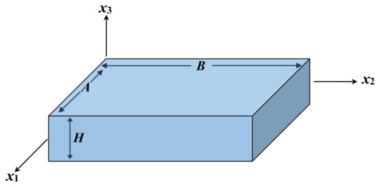
Figure 1.
Configuration and coordinates of a porous nanocomposite plate.
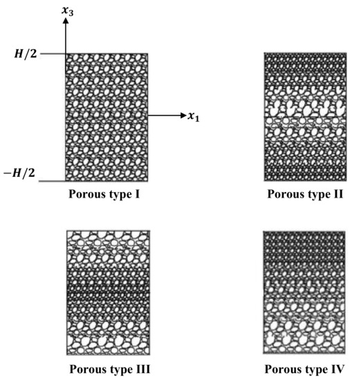
Figure 2.
Porosity distribution types.
The effective mechanical and piezoelectric characteristics of porous nanocomposite plates as functions of are given as follows by the closed-cell cellular solids [28,29]:
in which , , , and denote Young’s modulus, the thermal expansion coefficient, the piezoelectric coefficients, the dielectric coefficients and Poisson’s ratio of the nanocomposite structures without porosity, respectively. Furthermore, according to Kitipornchai et al. [29], the mass density coefficient is presented in terms of the porosity coefficient as:
and
The shear modulus of the plates with pores is
Next, using the Halpin–Tsai micromechanics model and the mixture rule [30,31,32,33], it is possible to predict the effective material properties of the FG GPLs-reinforced plates:
where , , and are Young’s modulus, mass density, Poisson’s ratio and thermal expansion coefficient of the GPLs (piezoelectric material), respectively. Moreover, the remaining properties, and denote the piezoelectric coefficients and the dielectric of the GPLs (piezoelectric material), respectively. However, the values for the parameters and are provided as [29]:
in which and denote the length, width and thickness of the GPLs, respectively.
In addition, there are four different GPLs distribution patterns, created by altering the volume fraction of the GPLs through the thickness of the plates according to a cosine distribution rule. The GPLs are evenly dispersed throughout the thickness for Pattern A. In contrast, the GPLs for Patterns B, C and D are functionally graded through the thickness, as shown in Figure 3. As a result, the volume fraction of GPLs can be expressed as follows [29]:
where are defined as the top values of GPLs volume fraction, which can be calculated as [29]:
where is the GPLs weight fraction.
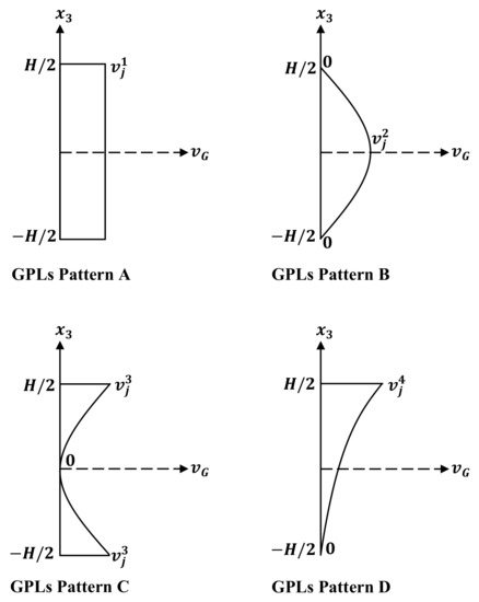
Figure 3.
GPLs distribution patterns.
3. Constitutive Equations
The two-variable shear deformation plate theory was first established for isotropic panels by Shimpi [34]. This theory has been extended for FG structures by many authors [35,36], and contains four variables and various shape functions. This theory considers the transverse shear effects and parabolic distribution of the transverse shear stresses through the thickness. Since the transverse shear strains and stresses are correctly represented, it is unnecessary to use shear correction factors. In addition, this theory satisfies the traction-free boundary conditions at the panel faces. Accordingly, a modified refined four-variable shear deformation theory [14,34,37] for FG porous GPLs-reinforced plates is presented to describe the displacement components as follows:
where and represent the components of the mid-plane displacements along the - and -axes, respectively. The deflection is separated into two components, and , which specify, respectively, the bending and the shear displacements, according to Shimpi’s theory [34] and . In addition, the shape function that describes the configuration of the shear stress along the thickness of the plate can be demonstrated by [15,34]:
The components of the strains can be calculated using the displacements field (9) as follows:
In terms of the piezoelasticity theory [3,38,39], the constitutive relationship for the components of the stresses can be described as follows:
where are the composite plate’s elastic coefficients, which are written as:
and denotes the applied temperature, which is supposed to be vary along the thickness of the plate according to the following law [32]:
where k indicates the temperature exponent. Furthermore, the electric displacements can be written as [38]:
According to [38], the electric field can be written as:
where represents the electric potential of the FG-GPLs/piezoelectric plate, which can be described as [38]:
in which is the external applied electric potential and denotes the electric potential of the middle surface of the plate. Equation (17) is substituted into Equation (16) to provide the components of the electric field as follows:
4. Governing Equations
To conclude the governing equations, we will use the principal of virtual work, which can be expressed as:
where the variation of the strain energy and the variation of the work done by the in-plane piezoelectric load and the external loads are given as follows:
in which q denotes the vertical load applied to the plate and denotes the in-plane piezoelectric load, which is defined as [38]:
5. Solution Procedure
5.1. Levy-Type Solution
In this section, the Levy-type approach [32,40] is employed here with respect to the variety of boundary conditions to reduce governing Equation (26) to a system of ordinary differential equations that can be solved exactly or approximately. However, Levy-type solution can be developed for rectangular nanoplates with at least two opposite edges that are simply supported, while the remaining two edges can have any possible combination of boundary conditions: free, simply supported or clamped. In accordance with this approach, the edges parallel to the -axis are assumed to be simply supported, given as:
The boundary conditions of the edges parallel to the -axis can have a combination of simply supported, clamped or free conditions, which can be expressed as [32]:
Simply supported (S):
Clamped (C):
Free (F):
The simply supported boundary conditions can be fulfilled by trigonometric functions in , and the resulting ordinary differential equations in can be solved by applying the state-space method or the differential quadrature method. According to the Levy solution process, we consider the following representation of the displacements and loading as follows [32]:
where . For the sinusoidal load, the functions and are expressed as:
5.2. Differential Quadrature Solution
In this section, Equation (33) is solved using the differential quadrature approach. The DQM is a common numerical method that has been implemented to solve initial and boundary value problems by many authors (see, e.g., [33,41]). In particular, the DQM predicts precise results using significantly fewer grid points when compared to traditional-order finite difference and finite element analysis (FEM) [42,43]. In accordance with the DQM, the sth-order partial derivatives of a function at a given discrete point i are approximated by putting a weighted linear sum of the function’s values over the entire domain; the nanocomposite plate is discretized by M mesh points. In particular, the sth-order derivative of a function at a given discrete point i can be given for M discrete grid points as follows [42]:
in which are the weighting coefficients associated with the sth derivative, which can be written for higher-order derivatives as [42]:
In contrast, the weighting coefficients associated with the first-order derivative is written as [42]:
Furthermore, in accordance with the Gauss–Chebyshev–Lobatto method, the distributed grid points are generated as follows [42]:
By applying the DQ approximation formulas (35)–(38) into Equation (33), the governing equations can be discretized and converted to linear algebraic equations as follows:
Furthermore, the boundary conditions can be expressed as follows in a discretization form:
Simply supported:
Clamped:
Free:
6. Numerical Results
Various numerical examples are introduced in the current section to illustrate the influences of different parameters such as porosity factor, porosity distribution types, GPLs weight fraction, GPLs distribution patterns, side-to-thickness ratio, temperature parameter, temperature exponent, external electric voltage and boundary conditions on the deflection and stresses of the FG porous piezoelectric plate reinforced with GPLs. For this purpose, the following quantities are defined:
The material properties of the piezoelectric matrix and GPLs are given in Table 1, noting that the parameter is named as the piezoelectric multiple [44].

Table 1.
Material properties of the piezoelectric matrix and GPLs [44].
The following fixed data (unless otherwise declared) are used in the numerical examples: Pa, m, m, m, nm.
Firstly, Table 2 displays a convergence study for the present results of the FG porous piezoelectric plate reinforced with GPLs. In this table, we determine the minimum number of mesh points required for converged solutions in the DQM. It is notable that 15 mesh points are sufficient to achieve a converged solution.
Table 2.
Convergence of the results of FG porous nanocomposite piezoelectric square plates.
Secondly, in order to check the accuracy of the results obtained by the current formulations, the present deflection () of an FG square plate is compared with those provided by Thai and Kim [45], as shown in Table 3. The FG plate is composed of ceramic (c) and metal (m) with the following properties: GPa, GPa, . The effective Young’s modulus is calculated as:
Table 3.
Comparison of the central deflection of an FGM square plate.
Moreover, the results in this table are given for different values of the side-to-thickness ratio and power law index . From Table 3, the present deflection is in good agreement with that obtained by Thai and Kim [45].
Table 4, Table 5, Table 6 and Table 7 depict the effects of the side-to-thickness ratio and GPLs weight fraction on the dimensionless central deflection , the normal stress , the transverse shear stress and the in-plane shear stress of FG porous nanocomposite piezoelectric square plates under various boundary conditions. It is observed that regardless of the type of boundary conditions, central deflection gradually increases with increasing side-to-thickness ratio . On the other hand, it decreases as the GPLs weight fraction increases. Furthermore, the sensitivity of the deflection to variations of the boundary conditions is very noticeable. It is notable that the plates with clamped edges have minimum values of normal and transverses stresses, while plates with free and clamped edges suffer more deflection and stresses. It can be also observed that the stresses , and decrease as the side-to-thickness ratio increases. They increase as the GPLs weight fraction increases, except the in-plane shear stress , which no longer increases as increases.
Table 4.
Dimensionless central deflection of FG porous nanocomposite piezoelectric square plates under various boundary conditions and for different values of side-to-thickness ratio and GPLs weight fraction .
Table 5.
Dimensionless normal stress of FG porous nanocomposite piezoelectric square plates under various boundary conditions and for different values of side-to-thickness ratio and GPLs weight fraction ().
Table 6.
Dimensionless transverse shear stress of FG porous nanocomposite piezoelectric square plates under various boundary conditions and for different values of side-to-thickness ratio and GPLs weight fraction ().
Table 7.
Dimensionless in-plane shear stress of FG porous nanocomposite piezoelectric square plates under various boundary conditions and for different values of side-to-thickness ratio and GPLs weight fraction ().
The effect of the porosity factor on the central deflection of FG porous nanocomposite piezoelectric square plates is plotted in Figure 4. Four different porosity distribution types—I, II, III and IV—are illustrated in the corresponding figures (a), (b), (c) and (d), respectively. The effect of the porosity factor on the central deflection is more pronounced for small values of , especially for Type I and IV. In contrast, the effect of on is minimum for large values of , especially for porosity Type II, since the thermal conductivity of the porosity is much lower than that of the composite materials. Therefore, increasing the porosity reduces the thermal effects on the plate. Subsequently, a noticeable reduction in the deflection occurs as the porosity factor increases, especially for Types I and III. However, for Type IV, the deflection behaves in an opposite manner to the variation of the porosity factor. Note that, at the top surface of the plate (Type IV), there is no porosity and the temperature is maximum (see, Equation (14)); then, the porosity linearly increases through the thickness; while the temperature linearly decreases () in the same direction. Therefore, the role of pores in reducing the effects of the temperature on the plate stiffness are very weak or may be missed because the temperature naturally decreases in the direction of increasing pores. Subsequently, the deflection increases as the porosity factor increases. This also explains the weak role of pores to reduce the deflection for Type II.
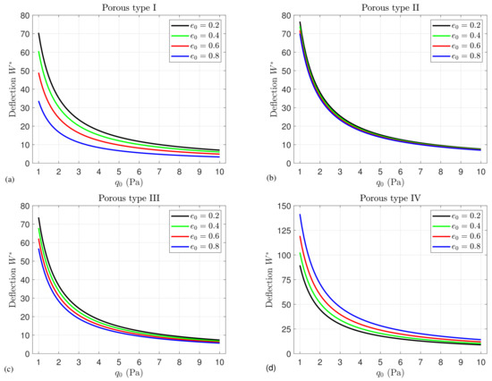
Figure 4.
Influence of the porosity factor on the central deflection of GPLs Pattern A of FG porous nanocomposite piezoelectric square plates for different porosity distribution types: (a) Type I, (b) Type II, (c) Type III and (d) Type IV.
For different porosity distribution Types I, II, III and IV, the impact of the porosity factor on the normal stress , transverse shear stress and in-plane shear stress through the thickness of FG porous nanocomposite piezoelectric square plates is illustrated in Figure 5, Figure 6 and Figure 7, respectively. It is obvious that, generally, for all porosity distribution types, the impact of the porosity factor on the normal stress , transverse shear stress and in-plane shear stress is significantly dependent on the porosity type. Moreover, for Type I, the porosity is uniformly distributed through the thickness; therefore, the plate becomes an isotropic structure. Accordingly, the normal stress and in-plane shear stress are linearly varied through the thickness of the plate, whereas the transverse shear stress is parabolically changed. It is found that the maximum normal stress decreases as the porosity factor increases. Note that for porosity distribution Types I and II, the maximum stress occurs at the bottom surface of the plate, while it occurs near the bottom surface for Types III and IV, as shown in Figure 5.
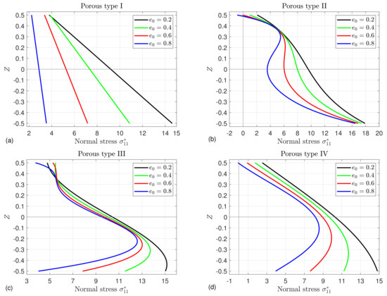
Figure 5.
Influence of the porosity factor on the normal stress in FG porous nanocomposite piezoelectric square plates for different porosity distribution types: (a) Type I, (b) Type II, (c) Type III and (d) Type IV.
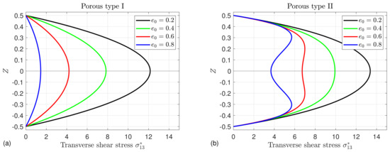
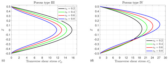
Figure 6.
Influence of the porosity factor on the transverse shear stress in FG porous nanocomposite piezoelectric square plates for different porosity distribution types: (a) Type I, (b) Type II, (c) Type III and (d) Type IV.
Figure 7.
Influence of the porosity factor on the in-plane shear stress in FG porous nanocomposite piezoelectric square plates for different porosity distribution types: (a) Type I, (b) Type II, (c) Type III and (d) Type IV.
In Figure 6a,c, the maximum transverse shear stress occurs at the mid-plane of the plate for all values of porosity factor . However, for Type IV, it occurs near the mid-plane of the plate, as shown in Figure 6d, because this type has an asymmetric porosity distribution. Since the volume fraction of porosity in Type II is maximum at the mid-plane (), the shear stress at is very sensitive to the variation of the porosity factor . Therefore, the stress has non-parabolic shapes for the largest values of . Note that for porosity distribution Types I, II and III, the maximum stress decreases with increasing , while for Type IV, it increases with the increase of .
It can be observed that for porosity distribution Types I, II and IV, the maximum in-plane shear stress occurs at the top surface of the plate, as shown in Figure 7, while for Type III, the maximum occurs near the top surface of the plate. Furthermore, for Types I, II and III, the maximum stress is decreased as the porosity factor increases. However, this trend is reversed for Type IV; increasing leads to the increase of the maximum stress .
To explain the impact of the GPLs weight fraction on the obtained results, the central deflection of FG porous nanocomposite piezoelectric square plates against transverse load is plotted in Figure 8 for various values of and for different graphene distribution patterns. In agreement with the review of the literature, the proportion of graphene in the plates greatly improves the mechanical properties of the plates and enhances their stiffness. Therefore, we notice a successive decreasing of the central deflection as the weight fraction increases.
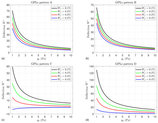
Figure 8.
Influence of the GPLs weight fraction on the central deflection of FG porous nanocomposite piezoelectric square plates for different graphene distribution patterns: (a) Pattern A, (b) Pattern B, (c) Pattern C and (d) Pattern D.
The Influence of the GPLs weight fraction on the normal stress , transverse shear stress and in-plane shear stress through the thickness of FG porous nanocomposite piezoelectric square plates is plotted in Figure 9, Figure 10 and Figure 11, respectively, for different graphene distribution patterns. We can clearly observe from Figure 9 that the maximum stress increases as the GPLs weight fraction increases. For more clarity, is linearly varied through the thickness of the plate for GPLs Pattern A (see Figure 9a), indicating the even distribution of GPLs through the plate thickness. In particular, for GPLs pattern B (see Figure 9b), the normal stress is nearly zero at the top and bottom surfaces of the plate, and the maximum occurs nearly at the mid-plane of the plate, because the GPLs weight fraction is maximum at the middle plane of the plate and equals to zero at the upper and lower faces. It is also notable that the normal stress in the upper part of the plate of Pattern B has extremums at the large values of (as shown in Figure 9b) due to the sensitivity of graphene to temperature, which has a maximum value at the top surface (see Equation (14)). Furthermore, since the temperature has small values in the lower part of the plate, the stress has no extremums in this part. Moreover, due to the asymmetric distribution of GPLs through the thickness of the plate of Pattern D (see, Figure 9d), the normal stress is zero at the bottom surface of the plate and is maximum at the top surface of the plate.
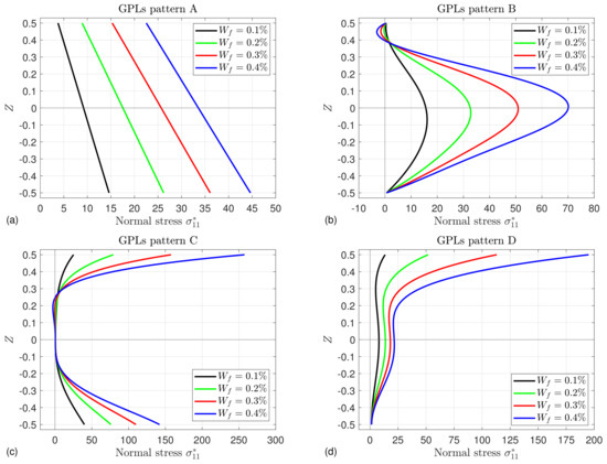
Figure 9.
Influence of the GPL weight fraction on the normal stress in FG porous nanocomposite piezoelectric square plates for different graphene distribution patterns: (a) Pattern A, (b) Pattern B, (c) Pattern C and (d) Pattern D.
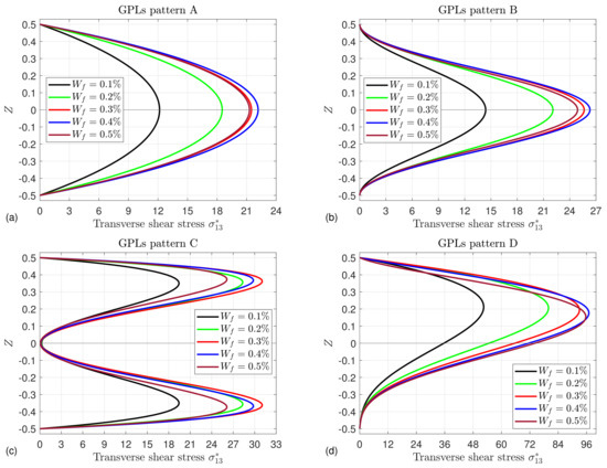
Figure 10.
Influence of the GPL weight fraction on the transverse shear stress in FG porous nanocomposite piezoelectric square plates for different graphene distribution patterns: (a) Pattern A, (b) Pattern B, (c) Pattern C and (d) Pattern D.
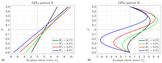
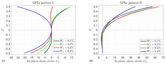
Figure 11.
Influence of the GPL weight fraction on the in-plane shear stress in FG porous nanocomposite piezoelectric square plates for different graphene distribution patterns: (a) Pattern A, (b) Pattern B, (c) Pattern C and (d) Pattern D.
It can be seen from Figure 10 that the stress of all GPL distribution patterns has the same behavior with the variation of . It increases to reach its maximum and then decreases as increases. These maximums depend on the GPL distribution pattern. This means that, adding more graphene to the structures makes the stress behave in an opposite sense, especially with considering the thermal load, since graphene possesses high thermal conductivity.
In addition, owing to the same reasons discussed in Figure 9b, the maximum stress in the upper part of the plate has the same distribution with the variation of for all patterns (see Figure 11); it no longer increases as the weight fraction increases, while, the maximum in the lower part of the plate increases monotonically as increases. Note that the positive and negative signs indicate the tensile and compressive stresses, respectively.
It is noteworthy that the stresses , and significantly depend on the volume fraction of GPLs , they equal zero when is equal to zero. Note that the volume fractions of GPLs patterns B, C and D are equal to zero at , and , respectively.
Figure 12 depicts the variation of the temperature parameter on the central deflection , normal stress , transverse shear stress and in-plane shear stress of FG porous nanocomposite piezoelectric square plates. As is well known, an increase in temperature weakens the structures, so the deflection and the shear stresses and increase monotonically as the temperature parameter increases. Moreover, the normal and shear stresses may be equal to zero at the top and bottom surfaces of the plate, indicating the significant dependence of the stresses on the GPLs volume fraction. Since the normal stress is directly dependent on the temperature (see Equation (12)), it is more sensitive to variation of the temperature and behaves differently from the shear stresses. Note that the temperature is maximum at the top surface of the plate and then decreases gradually to its minimum at the lower surface. Therefore, for small values of temperature ( = 50,100 or in the lower part of the plate), the maximum tensile stress decreases as the temperature parameter increases, while for large values of temperature (that occur in the upper part of the plate), the maximum compressive stress increases with the increase in temperature.
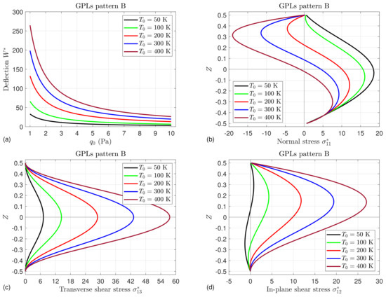
Figure 12.
Influence of the temperature parameter on the (a) central deflection , (b) normal stress , (c) transverse shear stress and (d) in-plane shear stress of FG porous nanocomposite piezoelectric square plates.
In Figure 13, the impact of the temperature exponent k on the central deflection , normal stress , transverse shear stress and in-plane shear stress of FG porous nanocomposite piezoelectric square plates is investigated. It can be observed that the temperature exponent k has a hardening effect. Accordingly, the deflection is decreased as k and increase. Furthermore, it is seen that for linear variation of the temperature (), the normal stress is also linearly changed through the thickness of the plate. The in-plane shear stress is linearly varied with respect to Z for all values of k. The shear stresses and decrease with increasing k, while this trend may be reversed for the normal stress, especially for .
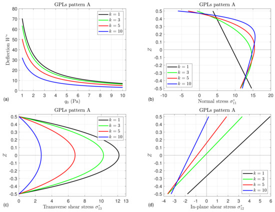
Figure 13.
Influence of the temperature exponent k on (a) the central deflection , (b) the normal stress , (c) the transverse shear stress and (d) the in-plane shear stress of FG porous nanocomposite piezoelectric square plates.
The influence of the applied electric voltage on the central deflection , the normal stress , the transverse shear stress and the in-plane shear stress of FG porous nanocomposite piezoelectric square plates is illustrated in Figure 14. The deflection decreases gradually as the electric voltage increases. This is reversed for the stresses; they increase as increases.
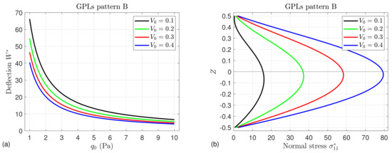
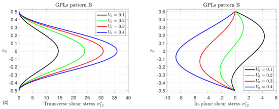
Figure 14.
Influence of the applied electric voltage on (a) the central deflection , (b) the normal stress , (c) the transverse shear stress and (d) the in-plane shear stress of FG porous nanocomposite piezoelectric square plates.
7. Conclusions
Levy-type solution and the DQM are utilized here to analyze the thermo-piezoelectric bending of FG porous piezoelectric plates reinforced with GPLs. The displacement field is formulated based on a refined four-variable shear deformation plate theory. To reduce the temperature effects, various types of porosity are considered in the present composite plate. This plate is composed of a piezoelectric material containing internal pores and is supported by FG GPLs. The differential equations are deduced by using the principle of virtual work including thermal, mechanical and electrical loads. These equations are converted to ordinary systems by using the Levy procedure and then discretized by the DQ method. The present formulations and theory are examined by comparing them to some examples from other research in the literature. Additional numerical results are presented to explain the effects of various parameters on the bending of the reinforced composite plates. Moreover, it is concluded that a considerable effect on the deflection and stresses is seen with variation of the edge boundary conditions. The deflection and stresses monotonically increase as the temperature parameter increases because elevated temperature leads to a reduction in the plate stiffness. The deflection decreases as the porosity factor, temperature exponent, transverse load, electric voltage and GPLs weight fraction increase. In addition, the maximum normal stresses decrease as the porosity factor increases. Increasing the electric voltage and the GPLs weight fraction leads to an increase in the shear stresses. The variation of the stresses through the thickness of the plate depends considerably on the porosity and GPLs distribution type. Furthermore, it can be concluded that with presence of a thermal load, adding a certain amount of graphene to structures enhances their toughness; consequently, a decrease in the deflection occurs. By adding more graphene, the structures become more flexible; accordingly, the deflection increases. To reduce the deformation of engineering structures caused by temperature, it is recommended to use structures reinforced with GPLs containing porosity, especially porosity Types I and III. However, it is not recommended to use porosity Type II or IV to reduce the thermal effect. The present results can be used as a benchmark for future investigations.
Author Contributions
Conceptualization, F.A., M.S. and F.H.H.A.M.; methodology, F.A., M.S. and F.H.H.A.M.; software, M.S.; validation, M.S.; formal analysis, F.A., M.S. and F.H.H.A.M.; investigation, F.A., M.S. and F.H.H.A.M.; resources, F.A., M.S. and F.H.H.A.M.; data curation, F.A., M.S. and F.H.H.A.M.; writing—original draft preparation, F.A., M.S. and F.H.H.A.M.; writing—review and editing, F.A., M.S. and F.H.H.A.M.; visualization, M.S. and F.H.H.A.M.; supervision, M.S. and F.H.H.A.M.; project administration, M.S. and F.H.H.A.M.; funding acquisition, F.A., M.S. and F.H.H.A.M. All authors have read and agreed to the published version of the manuscript.
Funding
This work was supported by the Deanship of Scientific Research, Vice Presidency for Graduate Studies and Scientific Research, King Faisal University, Saudi Arabia (Project No. GRANT1485), through its KFU Research Summer initiative.
Institutional Review Board Statement
Not applicable.
Informed Consent Statement
Not applicable.
Data Availability Statement
Not applicable.
Conflicts of Interest
The authors declare no conflict of interest.
References
- Wang, Z.; Chen, S.H.; Han, W. The static shape control for intelligent structures. Finite Elem. Anal. Des. 1997, 26, 303–314. [Google Scholar] [CrossRef]
- He, X.Q.; Ng, T.Y.; Sivashanker, S.; Liew, K.M. Active control of FGM plates with integrated piezoelectric sensors and actuators. Int. J. Solids Struct. 2001, 38, 1641–1655. [Google Scholar] [CrossRef]
- Sobhy, M. Piezoelectric bending of GPL-reinforced annular and circular sandwich nanoplates with FG porous core integrated with sensor and actuator using DGM. Arch. Civil Mech. Eng. 2021, 21, 1–18. [Google Scholar] [CrossRef]
- Wu, C.C.; Kahn, M.; Moy, W. Piezoelectric ceramics with functional gradients: A new application in material design. J. Amer. Ceram. S 1996, 79, 809–812. [Google Scholar] [CrossRef]
- El Harti, K.; Rahmoune, M.; Sanbi, M.; Saadani, R.; Bentaleb, M.; Rahmoune, M. Dynamic control of Euler Bernoulli FG porous beam under thermal loading with bonded piezoelectric materials. Ferroelectrics 2020, 558, 104–116. [Google Scholar] [CrossRef]
- Mallek, H.; Jrad, H.; Wali, M.; Dammak, F. Nonlinear dynamic analysis of piezoelectric-bonded FG-CNTR composite structures using an improved FSDT theory. Eng. Comp. 2021, 37, 1389–1407. [Google Scholar] [CrossRef]
- Zenkour, A.M.; Aljadani, M.H. Buckling analysis of actuated functionally graded piezoelectric plates via a quasi-3D refined theory. Mech. Mater. 2020, 151, 103632. [Google Scholar] [CrossRef]
- Moradi-Dastjerdi, R.; Behdinan, K. Free vibration response of smart sandwich plates with porous CNT-reinforced and piezoelectric layers. Appl. Math. Model. 2021, 96, 66–79. [Google Scholar] [CrossRef]
- Potts, J.R.; Dreyer, D.R.; Bielawski, C.W.; Ruoff, R.S. Graphene-based polymer nanocomposites. Polymer 2011, 52, 5–25. [Google Scholar] [CrossRef]
- Geim, A.K.; Novoselov, K.S. The rise of graphene. Nat. Mater. 2007, 6, 183–191. [Google Scholar] [CrossRef]
- Papageorgiou, D.G.; Kinloch, I.A.; Young, R.J. Mechanical properties of graphene and graphene-based nanocomposites. Prog. Mater. Sci. 2017, 90, 75–127. [Google Scholar] [CrossRef]
- Abolhasani, M.M.; Shirvanimoghaddam, K.; Naebe, M. PVDF/graphene composite nanofibers with enhanced piezoelectric performance for development of robust nanogenerators. Compos. Sci. Technol. 2017, 138, 49–56. [Google Scholar] [CrossRef]
- Mao, J.J.; Lu, H.M.; Zhang, W.; Lai, S.K. Vibrations of graphene nanoplatelet reinforced functionally gradient piezoelectric composite microplate based on nonlocal theory. Compos. Struct. 2020, 236, 111813. [Google Scholar] [CrossRef]
- Sobhy, M.; Al Mukahal, F.H.H. Analysis of Electromagnetic Effects on Vibration of Functionally Graded GPLs Reinforced Piezoelectromagnetic Plates on an Elastic Substrate. Crystals 2022, 12, 487. [Google Scholar] [CrossRef]
- Sobhy, M.; Al Mukahal, F.H. Wave Dispersion Analysis of Functionally Graded GPLs-Reinforced Sandwich Piezoelectromagnetic Plates with a Honeycomb Core. Mathematics 2022, 10, 3207. [Google Scholar] [CrossRef]
- Alazwari, M.A.; Zenkour, A.M.; Sobhy, M. Hygrothermal Buckling of Smart Graphene/Piezoelectric Nanocomposite Circular Plates on an Elastic Substrate via DQM. Mathematics 2022, 10, 2638. [Google Scholar] [CrossRef]
- Van Vinh, P.; Van Chinh, N.; Tounsi, A. Static bending and buckling analysis of bi-directional functionally graded porous plates using an improved first-order shear deformation theory and FEM. Eur. J.-Mech.-A/Solids 2022, 96, 104743. [Google Scholar] [CrossRef]
- Bot, I.K.; Bousahla, A.A.; Zemri, A.; Sekkal, M.; Kaci, A.; Bourada, F.; Tounsi, A.; Ghazwani, M.H.; Mahmoud, S.R. Effects of Pasternak foundation on the bending behavior of FG porous plates in hygrothermal environment. Steel Compos. Struct. 2022, 43, 821–837. [Google Scholar]
- Sahmani, S.; Aghdam, M.M.; Rabczuk, T. Nonlinear bending of functionally graded porous micro/nano-beams reinforced with graphene platelets based upon nonlocal strain gradient theory. Compos. Struct. 2018, 186, 68–78. [Google Scholar] [CrossRef]
- Amir, S.; Arshid, E.; Arani, M.R.G. Size-dependent magneto-electro-elastic vibration analysis of FG saturated porous annular/circular micro sandwich plates embedded with nano-composite face sheets subjected to multi-physical pre loads. Smart Struct. Syst. 2019, 23, 429–447. [Google Scholar]
- Barati, M.R.; Zenkour, A.M. Vibration analysis of functionally graded graphene platelet reinforced cylindrical shells with different porosity distributions. Mech. Adv. Mater. Struct. 2019, 26, 1580–1588. [Google Scholar] [CrossRef]
- Sobhy, M. Size dependent hygro-thermal buckling of porous FGM sandwich microplates and microbeams using a novel four-variable shear deformation theory. Int. J. Appl. Mech. 2020, 12, 2050017. [Google Scholar] [CrossRef]
- Sahmani, S.; Madyira, D.M. Nonlocal strain gradient nonlinear primary resonance of micro/nano-beams made of GPL reinforced FG porous nanocomposite materials. Mech. Based Des. Struct. Mach. 2021, 49, 553–580. [Google Scholar] [CrossRef]
- Zhao, S.; Yang, Z.H.; Kitipornchai, S.R.; Yang, J. Dynamic instability of functionally graded porous arches reinforced by graphene platelets. Thin-Walled Struct. 2020, 147, 106491. [Google Scholar] [CrossRef]
- Ansari, R.; Hassani, R.; Gholami, R.; Rouhi, H. Free vibration analysis of postbuckled arbitrary-shaped FG-GPL-reinforced porous nanocomposite plates. Thin-Walled Struct. 2021, 163, 107701. [Google Scholar] [CrossRef]
- Zenkour, A.M.; Aljadani, M.H. Buckling Response of Functionally Graded Porous Plates Due to a Quasi-3D Refined Theory. Mathematics 2022, 10, 565. [Google Scholar] [CrossRef]
- Raza, Q.; Qureshi, M.Z.A.; Ali, B.; Hussein, A.K.; Khan, B.A.; Shah, N.A.; Weera, W. Morphology of hybrid MHD nanofluid flow through orthogonal coaxial porous disks. Mathematics 2022, 10, 3280. [Google Scholar] [CrossRef]
- Roberts, A.P.; Garboczi, E.J. Computation of the linear elastic properties of random porous materials with a wide variety of microstructure. Proc. R. Soc. London. Ser. Math. Phys. Eng. Sci. 2021, 458, 1033–1054. [Google Scholar] [CrossRef]
- Kitipornchai, S.; Chen, D.; Yang, J. Free vibration and elastic buckling of functionally graded porous beams reinforced by graphene platelets. Mater. Des. 2017, 116, 656–665. [Google Scholar] [CrossRef]
- Halpin Affdl, J.C.; Kardos, J.L. The Halpin-Tsai equations: A review. Polym. Eng. Sci. 1976, 16, 344–352. [Google Scholar] [CrossRef]
- Rafiee, M.A.; Rafiee, J.; Wang, Z.; Song, H.; Yu, Z.Z.; Koratkar, N. Enhanced mechanical properties of nanocomposites at low graphene content. ACS Nano 2009, 3, 3884–3890. [Google Scholar] [CrossRef]
- Sobhy, M. Levy solution for bending response of FG carbon nanotube reinforced plates under uniform, linear, sinusoidal and exponential distributed loadings. Eng. Struct. 2019, 182, 198–212. [Google Scholar] [CrossRef]
- Sobhy, M. Differential quadrature method for magneto-hygrothermal bending of functionally graded graphene/Al sandwich curved beams with honeycomb core via a new higher-order theory. J. Sandw. Struct. Mater. 2021, 23, 1662–1700. [Google Scholar] [CrossRef]
- Shimpi, R.P. Refined plate theory and its variants. AIAA J. 2002, 40, 137–146. [Google Scholar] [CrossRef]
- Benachour, A.; Tahar, H.D.; Atmane, H.A.; Tounsi, A.; Ahmed, M.S. A four variable refined plate theory for free vibrations of functionally graded plates with arbitrary gradient. Compos. Part Eng. 2011, 42, 1386–1394. [Google Scholar] [CrossRef]
- Thai, H.T.; Choi, D.H. An efficient and simple refined theory for buckling analysis of functionally graded plates. Appl. Math. Model. 2012, 36, 1008–1022. [Google Scholar] [CrossRef]
- Zenkour, A.M.; Sobhy, M. Axial magnetic field effect on wave propagation in bi-layer fg graphene platelet-reinforced nanobeams. Eng. Comput. 2022, 38, 1313–1329. [Google Scholar] [CrossRef]
- Ke, L.-L.; Wang, Y.-S.; Yang, J.; Kitipornchai, S. Free vibration of size-dependent magneto-electro-elastic nanoplates based on the nonlocal theory. Acta Mech. Sin. 2014, 30, 516–525. [Google Scholar] [CrossRef]
- Zhang, S.; Xia, R.; Lebrun, L.; Anderson, D.; Shrout, T.R. Piezoelectric materials for high power, high temperature applications. Mater. Lett. 2005, 59, 3471–3475. [Google Scholar] [CrossRef]
- Sobhy, M. Levy-type solution for bending of single-layered graphene sheets in thermal environment using the two-variable plate theory. Int. J. Mech. Sci. 2015, 90, 171–178. [Google Scholar] [CrossRef]
- Al Mukahal, F.H.H.; Sobhy, M. Wave propagation and free vibration of FG graphene platelets sandwich curved beam with auxetic core resting on viscoelastic foundation via DQM. Arch Civil. Mech. Eng. 2022, 22, 1–21. [Google Scholar] [CrossRef]
- Shu, C. Differential Quadrature and Its Application in Engineering; Springer: Berlin/Heidelberg, Germany, 2012. [Google Scholar]
- Nateghi, A.; Salamat-Talab, M. Thermal effect on size dependent behavior of functionally graded microbeams based on modified couple stress theory. Compos. Struct. 2013, 96, 97–110. [Google Scholar] [CrossRef]
- Mao, J.J.; Zhang, W. Buckling and post-buckling analyses of functionally graded graphene reinforced piezoelectric plate subjected to electric potential and axial forces. Compos. Struct. 2019, 216, 392–405. [Google Scholar] [CrossRef]
- Thai, H.T.; Kim, S.E. A size-dependent functionally graded Reddy plate model based on a modified couple stress theory. Compos. Part B 2013, 45, 1636–1645. [Google Scholar] [CrossRef]


Publisher’s Note: MDPI stays neutral with regard to jurisdictional claims in published maps and institutional affiliations. |
© 2022 by the authors. Licensee MDPI, Basel, Switzerland. This article is an open access article distributed under the terms and conditions of the Creative Commons Attribution (CC BY) license (https://creativecommons.org/licenses/by/4.0/).