Abstract
With the development of the “Internet +” model and the sharing economy model, the “online car-hailing” operation model has promoted the emergence of “online-hailing agricultural machinery”. This new supply and demand model of agricultural machinery has brought greater convenience to the marketization of agricultural machinery services. However, although this approach has solved the use of some agricultural machinery resources, it has not yet formed a scientific and systematic scheduling model. Referring to the existing agricultural machinery scheduling modes and the actual demand of agricultural production, based on the idea of resource sharing, in this research, the soft and hard time windows were combined to carry out the research on the dynamic demand scheduling strategy of agricultural machinery. The main conclusions obtained include: (1) Based on the ideas of order resource sharing and agricultural machinery resource sharing, a general model of agricultural machinery scheduling that meet the dynamic needs was established, and a more scientific scheduling plan was proposed; (2) Based on the multi-population coevolutionary genetic algorithm, the dynamic scheduling scheme for shared agricultural machinery for on-demand farming services was obtained, which can reasonably insert the dynamic orders on the basis of the initial scheduling scheme, and realize the timely response to farmers’ operation demands; (3) By comparing with the actual production situation, the path cost and total operating cost were saved, thus the feasibility and effectiveness of the scheduling model were clarified.
Keywords:
agricultural machinery scheduling; online-hailing agricultural machinery; co-evolutionary genetic algorithm; dynamic demand analysis MSC:
90B06
1. Introduction
As the application of Internet technology in agricultural production continues to expand, online appointment of agricultural machinery provides a new channel for achieving operational agreements between supply and demand parties [1,2]. “Machine owners” and “machine users” use online agricultural machinery APP to release operation supply and demand information to form order matching, which helps to promote the rational allocation of agricultural resources in the market. Although this method promotes “machine owners” and “machine users” to use the Internet to match supply and demand, the order matching mode is decentralized and lacks scientific guidance for continuous operation of farmers. The scheduling plan is drawn up by agricultural machine drivers themselves and lacks systematic consideration of agricultural machinery resources and operation demand. As the operation links of agricultural machinery operation services continue to extend, the demand for on-demand farming services will also increase. It is difficult for the existing scheduling method to scientifically dispatch the dispersed agricultural machinery resources to achieve the on-demand farming services that satisfy farmers. Therefore, it is necessary to explore the agricultural machinery scheduling method of an agricultural machinery service organization based on order resource sharing and agricultural machinery resource sharing for the intensive development of agricultural machinery resource utilization and the improvement of the on-demand farming services level.
Machinery scheduling is one of the key tasks in agricultural machinery management [3], and scholars have conducted a lot of research on the agricultural machinery scheduling problem from different perspectives and have achieved fruitful results. Basnet et al. (2006) proposed an agricultural machinery scheduling model for multi-farm crop harvest, and designed a heuristic algorithm based on greedy algorithm and taboo search algorithm and solved it [4]. Ferrer, J. C. et al. (2008) proposed a mixed-integer linear programming model to optimize grape-harvesting operations. In addition to human and mechanical costs and other resource constraints, they incorporated the grape quality into the model through the concept of quality loss function, and obtained the route of the grape harvesting operation based on this model. Their study showed that the proposed model could be used to support grape harvest planning in a large vineyard, at both a tactical and operational level [5]. Guan S et al. (2009) proposed a long-term resource allocation scheduling method based on a two-stage metaheuristic algorithm based on simulated annealing (SA), genetic algorithm (GA), and hybrid Petri network models. This method takes into consideration the time, mechanical, and labor resource limitations of each crop agricultural operation, and obtained a high resource utilization rate in a simulated sugarcane production process [6]. Orfanou et al. (2013) proposed a planning method for the sequential tasks of biomass collection and processing operations, and the operation plan and the total operating cost for each machine can be obtained by using this method [7]. Pengfei He et al. (2018) proposed an operational model to determine the optimal combine-harvesters’ scheduling for fragmental farmlands to minimize the wheat harvesting period, in which the minimum difference in the harvest time between the combine harvesters was used as the constraint. They proposed a hybrid tabu search method to solve the model to minimize the harvest period [8].
The essence of agricultural machinery scheduling is a resource scheduling problem of agricultural machinery supply and farmland operation demand with space-time characteristics and resource constraints, and a large number of studies have shown that the agricultural machinery scheduling problem can be transformed into a VRP problem with time windows for solution. The VRP problem studies how to arrange routes for vehicles to transport goods from the depot to multiple geographically dispersed customer points or to transport goods back to the depot under certain constraints [9]. In recent years, the expansion of basic VRP problem has gained wide attention, such as dynamic vehicle routing problem [10], vehicle routing problem with stochastic demand [11], simultaneous delivery-pickup problem [12], and green vehicle routing problem [13]. Reinforcement learning [14], neighborhood search [15], ant colony algorithm [16], and taboo search algorithm [17] have also been applied to the solution of the VRP problem. Many scholars have developed the research of agricultural machine scheduling problem based on the VRP problem. Lin et al. (2019) developed an optimization model to maximize farmers’ profits by optimizing the selection and harvesting plan of agricultural machinery. The model quantifies the trade-offs between crop yield, drying, and equipment selection in harvest decisions, and can provide decision support to crop and market information for individual farms in different regions [18]. Pitakaso and Sethanan (2019) developed the ALNS meta-heuristic algorithm to solve the machinery harvest scheduling problem with time windows to maximize the total area of shared infield resource system [19]. Zuniga et al. (2021) established an optimization model for farm production planning and mechanical scheduling to maximize farmers’ benefits, which takes into consideration the multi-crop production planning, multi-machinery scheduling, and crop rotation over a certain period of time [20]. Ma et al. (2021) studied the agricultural machinery scheduling problem of agricultural machinery cooperatives based on a cross-regional operation model, and developed a mathematical model for multi-objective planning with the lowest total cost and the highest service punctuality by considering multiple agricultural machinery points, multiple types, operation time windows, and spatial distances [21]. Chen et al. (2021) took agricultural machinery scheduling in a major epidemic as their research object, and analyzed the various costs of agricultural machinery scheduling, and established a model of agricultural machinery scheduling with the minimum total scheduling cost as the optimization objective [22]. Liang Zheng (2022) proposed a multi-objective particle swarm optimization algorithm suitable for modern agricultural machinery task scheduling, and designed an agricultural machinery operation and maintenance management system, and realized the task scheduling based on this algorithm, which optimized the operation time, operation cost, and operation quality of agricultural machinery [23]. Wang and Huang (2022) studied the harvester scheduling problem with an operator assignment joint, and developed a mixed-integer linear programming model that minimizes the total operation time and cost by determining the combination of the harvester and the operator and the route of the harvester [24]. In order to save production costs, improve the utilization of agricultural machinery and equipment and expand the scale of operation, agricultural production pays much attention to the common utilization and equipping of agricultural machinery. The agricultural machinery sharing model is particularly suitable for small-scale agricultural operators, especially crop farms [25]. Graf Plessen (2019) proposed a solution to the path planning problem based on crop allocation. This method not only offers the allocation scheme of machinery, but also maintains the flexibility of agricultural machinery scheduling among various areas of farmland, which is of great practical significance for large farms sharing machinery [26]. Wang and Huang (2022) proposed a new two-step scheduling framework for shared agricultural machinery with time windows and applied it to an agricultural machinery service organization [27].
Static scheduling of agricultural machinery has received extensive attention and research. However, agricultural field operations form a dynamic and complex process [28], in which factors such as agricultural machinery breakdowns, weather, and roads make it impossible to execute the original plan by changing the supply or demand of agricultural machinery operation services. Some scholars have incorporated dynamic factors in the study of agricultural machinery scheduling. For example, Seyyedhasani H et al. (2018) discussed the impact of dynamic changes, such as vehicle number, work efficiency, and work area on operations in farmland [28]. Hu Y et al. (2020) considered the dynamic adjustment, which is the interruption of the original planning caused by agricultural machinery failure [29]. Cao et al. (2021) considered the dynamic task assignment in two scenarios of new task and agricultural machinery failure [30]. However, the dynamic scheduling strategy of agricultural machinery still needs further research, such as the dynamic scheduling strategy of agricultural machinery based on sharing mode. The dynamic scheduling of agricultural machinery can refer to the research ideas and research methods of dynamic vehicle scheduling, which are often transformed into problems of static vehicle scheduling [31,32,33]. Since the dynamic vehicle scheduling problem puts higher demand on efficiency and timeliness, and the exact algorithm is time-consuming, heuristic algorithms are mostly applied to solve this problem, such as taboo search (TS) [34], neighborhood search (NS) [35], ant colony optimization (ACO) [36], genetic algorithm (GA) [37], particle swarm optimization (PSO) [38], and hybrid algorithm [39,40]. Recently, reinforcement learning [41], artificial bee colony algorithms [42], and intelligent auction mechanisms [43] have also been applied to solve problems in dynamic vehicle scheduling.
Starting from the perspective of sharing and integrated utilization of existing agricultural machinery resources, by weakening the affiliation between orders, agricultural machinery, and agricultural machinery service organizations, this research was conducted to explore a new farming operation mode for mutual assistance with agricultural machinery, equipment sharing, and mutual benefit between agricultural machinery service organizations. Meanwhile, the general model of agricultural machinery scheduling with dynamic demand was established by integrating the influencing factors and characteristics of agricultural machinery scheduling process. The main contributions of this paper include:
- (1)
- Taking the principles and methods of system engineering as the core idea, and based on the theory of multi-depot scheduling, a general mathematical model of agricultural machinery scheduling with dynamic demand was established with the sharing mode of order resources and agricultural machinery resources. According to the priority of dynamic operation requirements, a scheduling strategy for real-time insertion of emergency orders and batch insertion of non-emergency orders was proposed;
- (2)
- The algorithm of solving the model was improved and designed, and the heuristic decoding operation was used to distribute the operation requirements according to the priority of agricultural machinery points, so as to reduce the total distance of agricultural machinery scheduling as a whole.
2. Proposal of Research Questions and Construction of Scheduling Model
2.1. Description of the Research Problem
Since farmers’ operation demands are from different farmlands and need to meet different operation time windows, agricultural machinery service organizations (such as agricultural machinery cooperatives, etc.) provide on-demand services for farmers through reasonable scheduling of shared agricultural machinery. The agricultural machinery scheduling problem based on the sharing model studied in this paper is mainly aimed at the agricultural machinery service model oriented to operation order demand with agricultural machinery service organizations (such as agricultural machinery cooperatives, etc.) as the agricultural machinery resource provider. The problem of agricultural machinery scheduling in this model can be described as: if there are different models of agricultural machinery at different locations in the current area, the operators need to go to different operation points to complete the operation, and the newly arrived operation order needs to be processed online during the operation at the same time. Therefore, a scheduling strategy is needed to allocate suitable models for each farmland operation point and to arrange a suitable operation route so that the agricultural machinery can complete the order tasks on time at the lowest cost. The dispatch network diagram is shown in Figure 1.
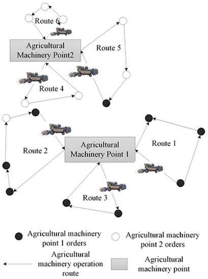
Figure 1.
Network diagram of agricultural machinery scheduling in resource sharing mode.
Therefore, the operation order included in the scheduling problem consists of two parts:
- (1)
- The initial order: The initial order is the integration of two parts of the order. One part is the operation needs of the cooperative itself, the other part includes the orders that has been accepted by the beginning of the first operation period and the operation orders that have not been inserted in the previous working day;
- (2)
- Dynamic orders: Dynamic orders are the orders that temporarily reach the scheduling center during the agricultural machinery operation process.
2.2. Assumptions of the Model
Combined with the needs of the actual investigation and theoretical analysis, the relevant assumptions for model construction are given as follows:
- (1)
- The geographic locations of agricultural machinery points at different locations in the scheduling area are known and fixed;
- (2)
- Each agricultural machinery point maintains different models of agricultural machinery and the quantity of each model of agricultural machinery is known. The operating power and operating cost of the same model of agricultural machinery are also known. The impact of the agricultural machinery’s service life on operating power is not considered for the time being;
- (3)
- The geographical location, working area, and working time window of the farmland in the order submitted by the farmer are all known, and the distances between all agricultural machinery points and farmland working points are known;
- (4)
- The needs of each operating point must be met and can only be accessed once by one agricultural machine. In order to standardize the management and maintenance of agricultural machinery, as well as the calculation of subsequent operation revenue, each agricultural machinery starts from the agricultural machinery point and needs to return to the agricultural machinery point after completing the task of the day;
- (5)
- In the process of generating the initial plan, it is assumed that the number of agricultural machinery participating in the scheduling is enough to be allocated for each operation path;
- (6)
- The agricultural machinery in the model does not have a capacity limit. The research objective is only for operating agricultural machinery. The operating time of agricultural machinery is composed of the transfer time between operating points and the operating time at operating points. The total daily working time of agricultural machinery was set to 10 h, and the inflow of materials and the output of agricultural products were not considered for the time being.
In actual investigation, it was found that the operating power of agricultural machinery at this stage can well meet the operating needs of farmers. If the span of the time window is too long, the operating time of the agricultural machinery will be included in the range of the time window; if the span of the time window is shortened, multiple changes to the scheduling plan will cause confusion in the agricultural machinery path. Based on the working hours of agricultural machinery operations, in this study, the agricultural machinery operating hours were divided into five discrete time windows, with each time window lasting for 2 h, so that an ideal order response state can be achieved. The division of the time windows is shown in Table 1.

Table 1.
Division of the five scheduling periods.
2.3. Model Establishment
Aiming at the characteristics of this problem, a mixed-integer linear programming model for agricultural machinery scheduling with time window constraints for multi-depot, multi-model, and dynamic demands vehicle routing was established to solve the actual problem of agricultural machinery scheduling. Define as a complete graph that can completely represent the system composed by the problem. The symbols and their meanings involved in the model are as follows:
- (1)
- Collection
is the collection of all nodes, and , including agricultural machinery points of the agricultural machinery cooperatives and all farmland operation points;
is the collection of depots, and representing depots in number, and the agricultural machinery point of each agricultural machinery cooperative is regarded as a depot in this study;
is the collection of all customers, and , representing customers in number (farmland operation points);
is the set of all paths, and ;
is a collection of all models of agricultural machinery owned by all agricultural machinery cooperatives in the area, and ;
- (2)
- Parameters
: The total amount of agricultural machinery in agricultural machinery points;
: Working hours of each agricultural machine;
: The driving time of agricultural machinery from operating point to operating point ;
: Operating hours of agricultural machinery at operating point ;
: The cost per unit distance traveled by agricultural machinery;
: The transfer speed of agricultural machinery;
: The number of agricultural machinery of the same model that has been used;
: Operation efficiency of the model of agricultural machinery ;
: Accumulative work volume of agricultural machinery at current operating point ;
[ei, li]: The time window of the operation point i, namely, the earliest operation start time and the scheduled completion time allowed by the operation point i.
- (3)
- Variables
is a 0–1 decision variable, indicating that the service at operation point is provided by the agricultural machinery ;
is a 0–1 decision variable, which means that if the agricultural machinery travels directly from the operating point to the operating point and starts to provide services, then , otherwise ;
The first stage: Path planning is performed on the received orders with the shortest agricultural machinery driving path as the objective function. During this process, the agricultural machinery tasks are arranged strictly according to the time window in the order. The objective function is:
Based on the actual situations and model assumptions of the agricultural machinery scheduling problem, the following constraints were established:
- (1)
- The number of agricultural machinery owned by each agricultural machinery point is limited, and the number of dispatched agricultural machinery cannot exceed the total amount of agricultural machinery owned by the agricultural machinery point.
- (2)
- One set of agricultural machinery can only provide services for one operation point, namely:
- (3)
- The needs of each operation point can be met, and can only be served by one set of agricultural machinery once, and multiple services from multiple agricultural machinery is not accepted, namely:
- (4)
- Each agricultural machine cannot travel between the agricultural machinery points after departure, otherwise, the route between the agricultural machinery points is invalid. It can only go to the operating point, namely:
- (5)
- The agricultural machinery must leave the operating point right after completing the task at the current operating point, namely:
- (6)
- The agricultural machinery starts from the agricultural machinery point and cannot be parked at will after completing the tasks at each operation point, or if the agricultural machinery is parked at other agricultural machinery points, it must return to the agricultural machinery point of departure, namely:
- (7)
- The path planning of agricultural machinery should meet the time window requirements of the farmers to which the initial order belongs, and cannot be violated in non-emergency situations, namely:where is the time when agricultural machinery starts the operation at operation point .
- (8)
- The time window for agricultural machinery from the current operating point to the next operating point should meet the following conditions, namely:where is a very large positive number.
- (9)
- The total operation time of each agricultural machinery on the day should meet the following conditions, and the sum of the traveling time and operation time of the agricultural machine on the day cannot exceed the specified working hours, namely:
The workload of agricultural machinery at the operating point satisfies the following relationship, namely:
The second stage: When the agricultural machinery leaves the agricultural machinery point for farmland operations, the new orders received are taken as optional tasks, and the farmers who enjoyed the most services are the objective function of the current stage to maximize the operating area. When the initial time window and operating constraints are met, it is inserted into the current route of the agricultural machinery. In this process, the time window of the new order is used as a soft time window. If it can meet the working area requirements of the current route, the new order will be inserted, otherwise the insertion will be rejected, and the order will be reserved as the order waiting for the next working day for planning. The dynamic scheduling process of agricultural machinery is shown in Figure 2.

Figure 2.
Schematic diagram of the agricultural machinery dynamic scheduling process.
Assume that is the operation sequence of the first operation point in each period of the day, as shown in Table 2.
Table 2.
Insert position of new order.
The defined variables and parameters are as follows:
- (1)
- Collection
is the work point to be inserted into the path in all new orders;
- (2)
- Parameters
: The traveling time of agricultural machinery from operating point to operating point ;
: Operating hours of agricultural machinery at operating point ;
: The time when the agricultural machinery starts operation at operation point ;
: The time when the agricultural machinery arrives at operation point ;
: The time when the agricultural machinery arrives at operation point .
- (3)
- Variables
are binary variables, indicating whether the operation point is inserted into the operation task queue of the scheduling plan. If the insertion operation is accepted, the variable value is 1, and if the insertion operation is rejected, the variable value is 0.
The number of operating points inserted in the initial plan is the largest, and the objective function is:
On the basis of the initial scheduling plan in this paper, the path is divided into five time periods according to the workable time, and the operation points that are involved in the planning are divided into four insertable spaces. Therefore, constraints for these four parts and the entire path were set.
Restrictions:
- (1)
- In sections , the agricultural machinery starts from the operating point , but should not return to the operating point , and the agricultural machinery must end at the operating point and cannot leave the operating point , namely:
In the sections, the time when the agricultural machinery reaches the operating point must be earlier than the upper bound of the time window of the operating point , namely:
Referring to the above model, the constraint bar equations at , and can be obtained. In the planning of the entire path, an inserted operation point can only be inserted into one time period, to avoid repeated insertion.
- (2)
- Avoid inserting the same operation task repeatedly in different time periods.
- (3)
- Ensure that an operation task is executed at most once in the entire path.
3. Model Solving Algorithm Analysis
3.1. Selection of Model Solving Algorithm
From the analysis of the above-mentioned agricultural machinery scheduling problem, the agricultural machinery scheduling problem can be analyzed and solved on the basis of the dynamic multi-depot vehicle routing problem. Therefore, the solving process of the agricultural machinery scheduling is shown in Figure 3.
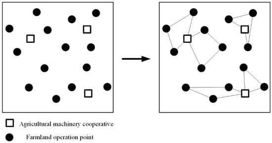
Figure 3.
Schematic diagram of solving agricultural machinery scheduling problem.
The meaning of the resource sharing model proposed in this paper is to realize the sharing of operation order resources and agricultural machinery resources among various agricultural machinery cooperatives. Therefore, the solution of the agricultural machinery scheduling problem cannot directly transform the multi-depot path optimization problem into the single-depot path optimization problem according to the principle of the nearest distance. The scheduling path planning should not only consider the distance between each operation point and the agricultural machinery center, but also according to the distance between the current position of the agricultural machinery and the location of the next operating point, in order to achieve the goal of minimizing the total scheduling cost. In view of the above characteristics, the idea of co-evolution was introduced into the genetic algorithm design, and then the co-evolution genetic algorithm was used to solve the problem. It is a kind of co-evolution algorithm that simulates the cooperative relationship between species in nature. It can not only overcome the shortcomings of the genetic algorithm itself, but also take into account the difficulties of multi-depot solution, in order to obtain a better agricultural machinery scheduling solution. In this paper, elite individuals and normal individuals are divided into different populations to evolve separately, and the individuals with a higher degree of adaptation appear in the evolution process to replace individuals with poorer performance of the next generation.
3.2. Design of the Scheduling Algorithm
In the process of designing the scheduling algorithm, it is necessary to input the position coordinate information of the agricultural machinery service organization, the parameter information such as the agricultural machinery model, the operation power and the activity cost, and the related information of the operation point location and the operation area. In addition, there are control parameters of co-evolutionary genetic algorithm, such as the elite population size, crossover probability and mutation probability. In this study, a multi-population coevolutionary genetic algorithm with elite strategy was used to divide the problem into one elite subpopulation and two ordinary subpopulations. Each subpopulation evolved its offspring population according to the prescribed cross probability and mutation probability, and finally the initial scheduling scheme that met the agricultural machinery operation ability and the order time window constraints were obtained; the nearest neighborhood search algorithm was used to plan the dynamic order according to the principle of the nearest distance between the new order and the current operation point of agricultural machinery, and the dynamic scheduling scheme was generated. For the selection of the agricultural machinery model, the improved saving algorithm was used to allocate the appropriate models according to the principle of minimum agricultural machinery power consumption per unit operation area, which should not violate the time window constraint of the initial order.
3.3. Multi-Population Coevolutionary Genetic Algorithm
3.3.1. Encoding and Decoding
The multi-population coevolutionary genetic algorithm was coded into integers, with being farming operation points and being agricultural machinery points. The initial population was obtained by random generation method. The decoding first determined the operation priority of farmland related to agricultural machinery points by the distance between farmlands and agricultural machinery points, and assigned farmland operation points to agricultural machinery points according to the operation priority. As shown in Figure 4, indicates the priority of operation point . The smaller means the higher priority of the operation point. After decoding, the operation order of agricultural machinery was obtained as 1-3-6-5-4-2-7.

Figure 4.
An instance of decoding.
3.3.2. Genetic Operation
The roulette selection operator was used in the selection operation, which is based on the fitness value to randomly select and retain the best individual in proportion.
The crossover operation used the sequential crossover method, as shown in Figure 5. The operation steps of sequential crossover are as follows.
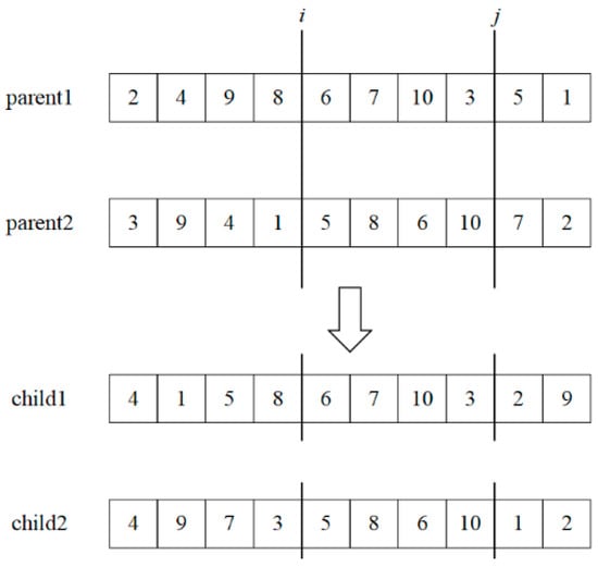
Figure 5.
An instance of the crossover operation.
Step 1: Select two chromosomes parent 1, parent 2 from the current population, and randomly select two positions , as crossover points to satisfy .
Step 2: The information of the operation point between positions and in chromosome parent1 was copied directly to the new offspring.
Step 3: Traverse from position in chromosome parent 2 to position , copy the operation point information from the chromosome parent 2 to the offspring that does not appear in the offspring.
Step 4: Swap the roles of two chromosomes to produce another offspring chromosome.
The exchange method was adopted in the mutation operation, which can only occur in the same route, and the process is shown in Figure 6. The steps of the mutation operation are as follows.
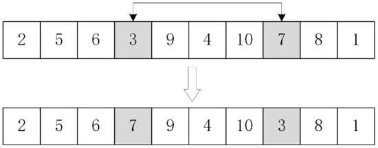
Figure 6.
An instance of the mutation operation.
Step 1: Generate a random number and . If takes a value less than the current mutation probability , then Step 2 is executed, otherwise, the mutation operation is not executed.
Step 2: Let the chromosome length be . Generate random integers , which represent the two positions of mutation in the same chromosome, and the genes at the two positions are exchanged.
Different mutation probabilities were used for different subpopulations. In order to avoid premature convergence and increase the population diversity brought by the mutation operation, the mutation probability was taken in an incremental strategy generation by generation at a later stage of the algorithm, i.e., after the 50th generation of evolution, the mutation probability increased by 0.001 per generation based on value setting.
3.3.3. Individual Evaluation
Individual evaluation is not isolated. On the contrary, they are combined with representative individuals from other populations in some way, and whether they are eliminated in evolution is determined by how well the combination of individuals performs in solving the target problem. As can be seen, the selection of cooperative representative individuals is a key aspect of information interaction between populations. In this paper, the inverse of the objective function was taken as the individual fitness value, and the greedy method was used to select the individual with the largest fitness value in the subpopulation as the representative individual to cooperate with other populations.
3.4. Algorithm Design of Dynamic Order Processing Strategy
The current distribution of rural land ownership determines that the operating area of unit orders is relatively small. When the number of orders generated reaches the peak during the operating season, the scheduling system is bound to reach a highly dynamic stage. Due to the limited time for decision-making in two consecutive periods, the adoption of real-time insertion strategy will save more scheduling time and computational cost, and it is not easy to cause confusion of traveling routes during the process of path transfer of agricultural machinery. Therefore, whenever a new request is received, the algorithm should try to find a feasible position to insert a new order without rescheduling the operation tasks that are already in the solution.
Whether new orders are received or not depends on the constraint of remaining operating capacity of the agricultural machinery, moreover, it generates operational costs and various events that occur during the traveling and operation of agricultural machinery, such as weather factors leading to extended operating time or poor road conditions leading to the decrease of traveling speed and the arrival of the new orders. In the face of real-time dynamic information, how to respond quickly and implement coping strategies is a key issue to improving operation efficiency. At the end of the period, orders that need to be executed during the period were received, and the order receiving and decision planning sequence is shown in Figure 7.

Figure 7.
The diagram of the order planning sequence.
By managing a planning set to respond to dynamic events in real time, some high-quality solutions were retained for the feasible solutions obtained by the algorithm. The structure of the planning set is shown in Table 3. Assuming that is the optimal solution in the current planning set, before the agricultural machinery starts to work, all the path schemes in the planning set are feasible, and these schemes are arranged according to the descending order of the total workload. Each time after completing the task at the operating point and before leaving for the next operating point, the agricultural machinery has to check whether the rest of the traveling route is feasible. In this way, the planning set will be updated after the agricultural machinery completes each operating task.
Table 3.
The structure of the planning set.
3.5. Algorithm Design of the Selection Strategy of the Operating Machine Model
The operation cost and operation power of different models of agricultural machinery are different, and the amount of operation tasks they can undertake is also different. In order to maximize the utility of existing agricultural machinery resources, an improved saving algorithm was used to determine the traveling route and the model of agricultural machinery. First we calculate the time saved by order insertion, as shown in Equation (23).
denotes the time that can be saved by inserting the operation point into the route where the operation point is located. denotes the traveling time between operation point and operation point (assuming that ). denotes the traveling time between agricultural machinery point and operation point . denotes the traveling time between agricultural machinery point and operation point .
is sorted by a descending order of values, and the optimization starts from the route associated with the maximum value of . If the new route satisfies the constraints of the problem without forming sub-routes and can satisfy the time window constraints as in Equation (24) below, the insertion of the new order can be accepted, otherwise it will be rejected.
denotes the time when agricultural machinery visits operation point , denotes the operation time of agricultural machinery at operation point , denotes the traveling time of agricultural machinery between operation point and operation point , and denotes the latest time allowed to start the operation at operation point .
The total amount of operation for route was compared with the operating power of each type of agricultural machinery and the final selection of agricultural machinery was made. Depending on the number of demands, if more than one model of agricultural machinery can be selected, the most economical choice is calculated as follows and the lowest is assigned to route .
denotes the power to be consumed by the agricultural machinery to complete the unit operation quantity; denotes the sum of all the operation quantities of route ; denotes the power of this model of agricultural machinery per unit time.
Since the amount of work that can be undertaken is different for different machinery models, the smaller the power required by the agricultural machinery to complete per unit of work, the more economical the scheduling scheme is. Therefore, different agricultural machinery-route matching combinations were calculated, and the solution with the path that contains the highest number of minimum is the optimal solution.
4. Empirical Analysis
4.1. Data Source and Collection
In this paper, three agricultural machinery professional cooperatives in Dujia Town, Wuchang City, Heilongjiang Province were taken as the research object, according to the actual situation of the investigation and related experimental data collected as instance analysis. The number of the cooperative is . The number and models of rice harvesters owned by each cooperative are shown in Table 4. There are 10 rice harvesters of all models, and the performance parameters and operation cost parameters of different models of harvesters are shown in Table 5. In the model simulation process, the total operation time of the harvester is 10 h/day. The traveling speed during the transfer of agricultural machinery is 35 km/h, and the transfer cost per unit distance is 2 CNY/km.
Table 4.
The number and models of agricultural machinery owned by each agricultural machinery cooperative.
Table 5.
The performance parameters and operation cost parameters of different models of agricultural machinery.
The whole scheduling problem will provide operation services to 50 operation points around the agricultural machinery cooperatives (36 operation points belonging to 3 cooperatives and 14 other operation points), of which the number of operation points that specified the operation orders is 36, and the coordinates and demand information are shown in Table 6.
Table 6.
Coordinates and operation information of cooperatives and work points.
4.2. Model Solving
In the rice harvest season, three agricultural machinery cooperatives collected the preliminary work orders. In the first stage of the solving algorithm, the crossover probability of the elite population was 0.9, the mutation probability was 0.05, the crossover probability of the ordinary population was 0.9, and the mutation probability was 0.1. In addition, after the 50th generation of the general population, the mutation probability increased by 0.001 per generation.
The relevant data and some variable values in the experiment process were brought into the model constructed in Section 2.3, and the MATLAB was used to program the algorithm to complete the simulation solution. The variation trend of the total cost of agricultural machinery scheduling in the first stage is shown in Figure 8. Figure 8 shows that, the objective function has stabilized after 140 generations of evolution.

Figure 8.
Cost trend chart of the initial scheduling scheme.
From the optimal results, it can be seen that the scheduling distance obtained by the scheduling plan is 98.7 km, the transfer cost is CNY 197.4, and the operating cost is CNY 9210.02. The scheduling path of the first stage is shown in Figure 9.
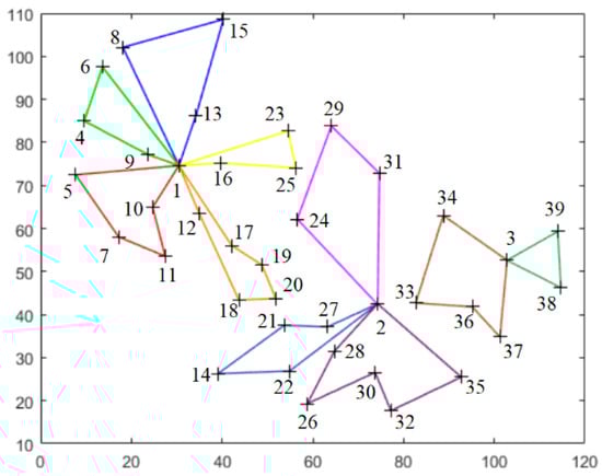
Figure 9.
The agricultural machinery scheduling path of the first stage.
In the second stage, 14 new orders during the 5 time periods in the actual production were summarized and substituted into the model. By optimizing and solving, a scheduling plan that can meet the time window requirements and the agricultural machinery operating capacity constraints is shown in Figure 10.

Figure 10.
The dynamic path of the agricultural machinery cooperatives in the second stage.
Based on the final scheduling scheme obtained by the dynamic scheduling stage, the completed operation area is 486.9 mu, and the operation cost is CNY 12,462.1.
5. Results and Analysis
5.1. Analysis of Optimal Scheduling Results
The scheduling path and operation sequence of each agricultural machinery are shown in Table 7. According to Figure 9 and Table 7, it can be seen that nodes 1–3 are the positions of the cooperatives, and nodes 4–39 are the positions of the farmlands to be operated in the cooperatives. In the first stage of the scheduling scheme, 18 operation points were assigned to agricultural machinery cooperative, 12 operation points were assigned to agricultural machinery cooperative, and 6 operation points were assigned to agricultural machinery cooperative, respectively. From the assignment of the operation points, it can be seen that the model is based on the target of the lowest operation cost. At the same time, it takes into account the completion of all the work areas under the premise of a given time window, which can be known from the work sequence and assigned work tasks. The task assignment of the model is balanced and can satisfy three cooperatives to complete their internal work tasks.
Table 7.
The first stage agricultural machinery scheduling path sequence.
In the second stage, 14 new orders were inserted to optimize the scheduling scheme to get the scheduling path and operation sequence of the agricultural machinery, as shown in Table 8.
Table 8.
The second stage agricultural machinery scheduling path sequence.
Referring to Figure 10 and Table 8, it can be seen that in the agricultural machinery operation process, the agricultural machinery cooperative received a total of six new orders, the agricultural machinery cooperative received a total of four new orders, and the agricultural machinery cooperative received a total of four new orders. After each agricultural machine received a new order, the traveling path of the agricultural machine has undergone new adjustments compared to the first stage. For example, for agricultural machinery H3, which started from the cooperative , when it received the first new insertion of order while carrying out the task at the first operation point 9, the model adjusted its position of operation according to the position of the order, so that it can meet the time window requirements while minimizing the operation cost. Table 8 shows the adjustment of the operation path after the insertion of new orders for the operation processes of other agricultural machinery. Among the optimization results, the agricultural machinery cooperatives with the largest number of agricultural machinery has the largest total operating area, and the agricultural machinery cooperatives with the least number of agricultural machinery has the smallest total operating area. It can be seen that the operating area of the cooperative matches its agricultural machinery ownership and agricultural machinery operating capacity. This shows that the scheduling strategy in this paper makes full use of the agricultural machinery resources of the three agricultural machinery cooperatives. This strategy not only avoids the waste of resources caused by idle agricultural machinery in larger-scale agricultural machinery cooperatives, but also avoids the delay in farming time caused by insufficient agricultural machinery resources in small-scale agricultural machinery cooperatives.
5.2. Comparative Analysis of Optimization Results and Actual Production
The results of the optimized scheduling are shown in Figure 11. In order to further clarify the feasibility and effectiveness of the scheduling model and scheme, the results of the optimized scheduling were compared with the actual production situation of three cooperatives in 2019. Since cooperatives mainly carry out production operation in the way of accomplishing their respective tasks in actual production, other order tasks can be accepted only after their own tasks are completed. Due to the limitation of production data collection in actual production, in this study, the total scheduling time, the path operation cost, and the total operation cost of the operating points of the three cooperatives were compared. The specific comparison is shown in Table 9.

Figure 11.
Visualization of the optimized scheduling.
Table 9.
Comparative analysis of the optimization results and the actual results.
It can be seen from Table 9 that the total scheduling time, the path operation cost, and the total operation cost of the scheduling scheme obtained by this optimized scheduling model were lower than the corresponding costs of scheduling based on experiences in the actual production of the cooperatives. The analysis results in Table 8 shows that the scheduling strategy can achieve the effect of operation distribution according to machine operation capacity. Therefore, this scheduling model is effective and feasible, and can be extended to a certain generalizability.
5.3. Suggestions
Combined with the research content, this paper has the following suggestions for the development of agricultural machinery service organization and agricultural machinery operation service:
- (1)
- Guide the agricultural machinery service organizations to change the mode of farming: all agricultural machinery service organizations should actively participate in the consortium of agricultural machinery service organizations to weaken the subordination among orders, agricultural machinery and agricultural machinery service organizations. In addition, these organizations should also explore the new agricultural operation mode of order sharing and agricultural machinery sharing among agricultural machinery service organizations, in order to achieve the reasonable use of agricultural machinery resources, reduce the agricultural machinery use cost, and mechanical loss;
- (2)
- Reasonable allocation of agricultural machinery resources of agricultural machinery service organizations: when purchasing agricultural machinery, agricultural machinery service organizations should be careful to purchase agricultural machinery with large quantity in the region, and increase the number of agricultural machinery with small quantity and increasing operation demand year by year;
- (3)
- Promote the orderly development of agricultural machinery operation services: strengthen the training and education of local farmers and agricultural machinery operators, promote and publicize agricultural machinery operation services in time, and guide agricultural machinery operators to participate in agricultural machinery operation services in an orderly manner, so as to improve the satisfaction of farmers and income of agricultural machinery operators.
6. Conclusions and Prospect
6.1. Conclusions
In view of the current situation of agricultural machinery scheduling under the “Internet +” mode, in order to realize the sharing of agricultural machinery based on the idea of cross-regional operation in multi-agricultural machinery cooperatives, to make full use of resources, reduce cost and increase efficiency, by analyzing the influencing factors in the process of agricultural machinery operation, the agricultural machinery scheduling model with dynamic demand based on order resource sharing and agricultural machinery resource sharing was established, and the hybrid heuristic algorithm was adopted to solve the scheduling model. Compared with the existing empirical scheduling method of agricultural machinery cooperatives, the scheme obtained in this paper optimized the operation order of agricultural machinery, and can realize the rapid response of farmers’ operation needs, so as to improve the level of on-demand farming services. The main conclusions are as follows:
- (1)
- Combined with the supply and demand scheduling situation of agricultural machinery under the “Internet +” mode, an agricultural machinery scheduling model based on order resource sharing and agricultural machinery resource sharing was proposed. Integrating the influencing factors and characteristics of the agricultural machinery scheduling process, a two-stage agricultural machinery scheduling model with dynamic demand was established. The model adopts a combination of soft time windows and hard time windows, as well as a scheduling strategy of real-time insertion of urgent orders and batch processing of dynamic demands;
- (2)
- According to the characteristics of the model, an optimized solving algorithm was designed. A multi-group co-evolutionary genetic algorithm with heuristic rules was used to generate the initial scheduling scheme, and according to the emergency status and priority rules of the order, the dynamic demand of the nearest neighborhood search strategy was inserted into the batch to process the new orders in each period. The saving algorithm was used to formulate the selection method of agricultural machinery model;
- (3)
- The effectiveness and feasibility of the scheduling strategy were verified and analyzed by the example simulation. Analyzing the rice harvesting operations in Wuchang City and comparing with the actual production data of three cooperatives, the effectiveness and feasibility of the model were verified.
6.2. Discussion of Future Research
- (1)
- The main objective of this study was to minimize the operation cost. It does not consider the matching problem between different operation areas and models of agricultural machinery, but different areas of farmland need to be assigned with matching models of agricultural machinery for operation. Therefore, the complexity of the model and problem solving are more difficult, which will be further improved in the follow-up research;
- (2)
- In the actual situation, the farmland segments are not isolated. How to schedule agricultural machinery to complete multiple tasks at the same time and the overall scheduling of operation and transport links need to be studied further;
- (3)
- This paper deals with the influencing factors in the operation scheduling process on the operation efficiency. For example, the influence of weather conditions is determined by the ratio of speed. However, the complexity of agricultural production is far more than this. It should involve the interaction between agricultural machinery systems and biological and meteorological subsystems such as crops, soil, and weather conditions, as well as the impact of several limiting factors on the performance of the entire operating system.
Author Contributions
Conceptualization, L.M. and Y.-J.W.; methodology, M.X. and Y.Z.; formal analysis, L.M. and Y.-J.W.; writing—original draft, L.M., M.X. and Y.Z.; writing—review and editing, L.M., M.X. and Y.-J.W.; supervision, L.M. and Y.-J.W. All authors have read and agreed to the published version of the manuscript.
Funding
This research was funded by the National Natural Science Foundation of China (52075091) and “Hundred, Thousand and Ten Thousand” Engineering Project of Heilongjiang Province (2019ZX14A04).
Data Availability Statement
The data presented in this study are available in article.
Conflicts of Interest
The authors declare no conflict of interest.
References
- Yang, H.; Xiong, S.; Frimpong, S.A.; Zhang, M. A Consortium Blockchain-Based Agricultural Machinery Scheduling System. Sensors 2020, 20, 2643. [Google Scholar] [CrossRef] [PubMed]
- Fountas, S.; Sørensen, C.G.; Tsiropoulos, Z.; Cavalaris, C.; Liakos, V.; Gemtos, T. Farm machinery management information system. Comput. Electron. Agric. 2015, 110, 131–138. [Google Scholar] [CrossRef]
- Bochtis, D.D.; Sørensen, C.G.; Busato, P. Advances in agricultural machinery management: A review. Biosyst. Eng. 2014, 126, 69–81. [Google Scholar] [CrossRef]
- Basnet, C.B.; Foulds, L.R.; Wilson, J.M. Scheduling contractors’ farm-to-farm crop harvesting operations. Int. Trans. Oper. Res. 2006, 13, 1–15. [Google Scholar] [CrossRef]
- Ferrer, J.-C.; Mac Cawley, A.; Maturana, S.; Toloza, S.; Vera, J. An optimization approach for scheduling wine grape harvest operations. Int. J. Prod. Econ. 2008, 112, 985–999. [Google Scholar] [CrossRef]
- Guan, S.; Nakamura, M.; Shikanai, T.; Okazaki, T. Resource assignment and scheduling based on a two-phase metaheuristic for cropping system. Comput. Electron. Agric. 2009, 66, 181–190. [Google Scholar] [CrossRef]
- Orfanou, A.; Busato, P.; Bochtis, D.; Edwards, G.; Pavlou, D.; Sørensen, C.; Berruto, R. Scheduling for machinery fleets in biomass multiple-field operations. Comput. Electron. Agric. 2013, 94, 12–19. [Google Scholar] [CrossRef]
- He, P.; Li, J.; Wang, X. Wheat harvest schedule model for agricultural machinery cooperatives considering fragmental farmlands. Comput. Electron. Agric. 2018, 145, 226–234. [Google Scholar] [CrossRef]
- Zhang, H.; Ge, H.; Yang, J.; Tong, Y. Review of Vehicle Routing Problems: Models, Classification and Solving Algorithms. Arch. Comput. Methods Eng. 2021, 29, 195–221. [Google Scholar] [CrossRef]
- Wang, Y.; Zhe, J.; Wang, X.; Fan, J.; Wang, Z.; Wang, H. Collaborative multicenter reverse logistics network design with dynamic customer demands. Expert Syst. Appl. 2022, 206, 117926. [Google Scholar] [CrossRef]
- Dinh, T.; Fukasawa, R.; Luedtke, J.R. Exact algorithms for the chance-constrained vehicle routing problem. Math. Program. 2018, 172, 105–138. [Google Scholar] [CrossRef]
- Park, H.; Son, D.; Koo, B.; Jeong, B. Waiting strategy for the vehicle routing problem with simultaneous pickup and delivery using genetic algorithm. Expert Syst. Appl. 2021, 165, 113959. [Google Scholar] [CrossRef]
- Sadati, M.E.H.; Çatay, B. A hybrid variable neighborhood search approach for the multi-depot green vehicle routing problem. Transp. Res. Part E Logist. Transp. Rev. 2021, 149, 102293. [Google Scholar] [CrossRef]
- Basso, R.; Kulcsár, B.; Sanchez-Diaz, I.; Qu, X. Dynamic stochastic electric vehicle routing with safe reinforcement learning. Transp. Res. Part E Logist. Transp. Rev. 2022, 157, 102496. [Google Scholar] [CrossRef]
- Yu, V.F.; Jodiawan, P.; Gunawan, A. An Adaptive Large Neighborhood Search for the green mixed fleet vehicle routing problem with realistic energy consumption and partial recharges. Appl. Soft Comput. 2021, 105, 107251. [Google Scholar] [CrossRef]
- Wang, Y.; Wang, L.; Chen, G.; Cai, Z.; Zhou, Y.; Xing, L. An Improved Ant Colony Optimization algorithm to the Periodic Vehicle Routing Problem with Time Window and Service Choice. Swarm Evol. Comput. 2020, 55, 100675. [Google Scholar] [CrossRef]
- Qiu, M.; Fu, Z.; Eglese, R.W.; Tang, Q. A Tabu Search algorithm for the vehicle routing problem with discrete split deliveries and pickups. Comput. Oper. Res. 2019, 100, 102–116. [Google Scholar] [CrossRef]
- Lin, T.; Liao, W.-T.; Rodríguez, L.F.; Shastri, Y.N.; Ouyang, Y.; Tumbleson, M.E.; Ting, K.C. Optimization Modeling Analysis for Grain Harvesting Management. Trans. ASABE 2019, 62, 1489–1508. [Google Scholar] [CrossRef]
- Pitakaso, R.; Sethanan, K. Adaptive large neighborhood search for scheduling sugarcane inbound logistics equipment and machinery under a sharing infield resource system. Comput. Electron. Agric. 2019, 158, 313–325. [Google Scholar] [CrossRef]
- Vazquez, D.A.Z.; Fan, N.; Teegerstrom, T.; Seavert, C.; Summers, H.M.; Sproul, E.; Quinn, J.C. Optimal production planning and machinery scheduling for semi-arid farms. Comput. Electron. Agric. 2021, 187, 106288. [Google Scholar] [CrossRef]
- Ma, L.; Wang, Y.; Ma, M.; Bai, J. Research on Multi-Cooperative Combine-Integrated Scheduling Based on Improved NSGA-II Algorithm. Int. J. Agric. Environ. Inf. Syst. 2021, 12, 1–21. [Google Scholar] [CrossRef]
- Chen, C.; Hu, J.P.; Zhang, Q.K.; Zhang, M.; Li, Y.B.; Nan, F.; Cao, G.Q. Research on the Scheduling of Tractors in the Major Epidemic to Ensure Spring Ploughing. Math. Probl. Eng. 2021, 2021, 3534210. [Google Scholar] [CrossRef]
- Zheng, L. Optimization of Agricultural Machinery Task Scheduling Algorithm Based on Multiobjective Optimization. J. Sens. 2022, 2022, 5800332. [Google Scholar] [CrossRef]
- Wang, Y.-J.; Huang, G.Q. Harvester scheduling joint with operator assignment. Comput. Electron. Agric. 2022, 202, 107354. [Google Scholar] [CrossRef]
- Larsen, K. Effects of machinery-sharing arrangements on farm efficiency: Evidence from Sweden. Agric. Econ. 2010, 41, 497–506. [Google Scholar] [CrossRef]
- Plessen, M.G. Coupling of crop assignment and vehicle routing for harvest planning in agriculture. Artif. Intell. Agric. 2019, 2, 99–109. [Google Scholar] [CrossRef]
- Wang, Y.-J.; Huang, G.Q. A two-step framework for dispatching shared agricultural machinery with time windows. Comput. Electron. Agric. 2022, 192, 106607. [Google Scholar] [CrossRef]
- Seyyedhasani, H.; Dvorak, J.S. Dynamic rerouting of a fleet of vehicles in agricultural operations through a Dynamic Multiple Depot Vehicle Routing Problem representation. Biosyst. Eng. 2018, 171, 63–77. [Google Scholar] [CrossRef]
- Hu, Y.; Liu, Y.; Wang, Z.; Wen, J.; Li, J.; Lu, J. A two-stage dynamic capacity planning approach for agricultural machinery maintenance service with demand uncertainty. Biosyst. Eng. 2020, 190, 201–217. [Google Scholar] [CrossRef]
- Cao, R.; Li, S.; Ji, Y.; Zhang, Z.; Xu, H.; Zhang, M.; Li, M.; Li, H. Task assignment of multiple agricultural machinery cooperation based on improved ant colony algorithm. Comput. Electron. Agric. 2021, 182, 105993. [Google Scholar] [CrossRef]
- Hong, L. An improved LNS algorithm for real-time vehicle routing problem with time windows. Comput. Oper. Res. 2012, 39, 151–163. [Google Scholar] [CrossRef]
- Schyns, M. An ant colony system for responsive dynamic vehicle routing. Eur. J. Oper. Res. 2015, 245, 704–718. [Google Scholar] [CrossRef]
- Okulewicz, M.; Mańdziuk, J. The impact of particular components of the PSO-based algorithm solving the Dynamic Vehicle Routing Problem. Appl. Soft Comput. 2017, 58, 586–604. [Google Scholar] [CrossRef]
- Ichoua, S.; Gendreau, M.; Potvin, J.-Y. Exploiting Knowledge About Future Demands for Real-Time Vehicle Dispatching. Transp. Sci. 2006, 40, 211–225. [Google Scholar] [CrossRef]
- Chen, S.; Chen, R.; Wang, G.-G.; Gao, J.; Sangaiah, A.K. An adaptive large neighborhood search heuristic for dynamic vehicle routing problems. Comput. Electr. Eng. 2018, 67, 596–607. [Google Scholar] [CrossRef]
- Montemanni, R.; Gambardella, L.M.; Rizzoli, A.E.; Donati, A.V. Ant Colony System for a Dynamic Vehicle Routing Problem. J. Comb. Optim. 2005, 10, 327–343. [Google Scholar] [CrossRef]
- Hanshar, F.T.; Ombuki-Berman, B.M. Dynamic vehicle routing using genetic algorithms. Appl. Intell. 2007, 27, 89–99. [Google Scholar] [CrossRef]
- Cortés, C.E.; Sáez, D.; Núñez, A.; Muñoz-Carpintero, D. Hybrid Adaptive Predictive Control for a Dynamic Pickup and Delivery Problem. Transp. Sci. 2009, 43, 27–42. [Google Scholar] [CrossRef]
- Elhassania, M.; Jaouad, B.; Ahmed, E.A. A new hybrid algorithm to solve the vehicle routing problem in the dynamic environment. Int. J. Soft Comput. 2013, 8, 327–334. [Google Scholar] [CrossRef]
- Barkaoui, M.; Gendreau, M. An adaptive evolutionary approach for real-time vehicle routing and dispatching. Comput. Oper. Res. 2013, 40, 1766–1776. [Google Scholar] [CrossRef]
- Anuar, W.K.; Lee, L.S.; Seow, H.-V.; Pickl, S. A Multi-Depot Dynamic Vehicle Routing Problem with Stochastic Road Capacity: An MDP Model and Dynamic Policy for Post-Decision State Rollout Algorithm in Reinforcement Learning. Mathematics 2022, 10, 2699. [Google Scholar] [CrossRef]
- Nagy, Z.; Werner-Stark, Á.; Dulai, T. An Artificial Bee Colony Algorithm for Static and Dynamic Capacitated Arc Routing Problems. Mathematics 2022, 10, 2205. [Google Scholar] [CrossRef]
- Zhang, J.; Zhu, Y.; Wang, T.; Wang, W.; Wang, R.; Li, X. An Improved Intelligent Auction Mechanism for Emergency Material Delivery. Mathematics 2022, 10, 2184. [Google Scholar] [CrossRef]


Publisher’s Note: MDPI stays neutral with regard to jurisdictional claims in published maps and institutional affiliations. |
© 2022 by the authors. Licensee MDPI, Basel, Switzerland. This article is an open access article distributed under the terms and conditions of the Creative Commons Attribution (CC BY) license (https://creativecommons.org/licenses/by/4.0/).