Abstract
(1) Background: Structuring is important in parallel programming in order to master its complexity, and this structuring could be achieved through programming patterns and skeletons. Divide-and-conquer computation is essentially defined by a recurrence relation that links the solution of a problem to the solutions of subproblems of the same type, but of smaller sizes. This pattern allows the specification of different types of computations, and so it is important to provide a general specification that comprises all its cases. We intend to prove that the divide-and-conquer pattern could be generalized such that to comprise many of the other parallel programming patterns, and in order to prove this, we provide a general formulation of it. (2) Methods: Starting from the proposed generalized specification of the divide-and-conquer pattern, the computation of the pattern is analyzed based on its stages: decomposition, base-case and composition. Examples are provided, and different execution models are analyzed. (3) Results: a general functional specification is provided for a divide-and-conquer pattern and based on it, and we prove that this general formulation could be specialized through parameters’ instantiating into other classical parallel programming patterns. Based on the specific stages of the divide-and-conquer, three classes of computations are emphasized. In this context, an equivalent efficient bottom-up computation is formally proved. Associated models of executions are emphasized and analyzed based on the three classes of divide-and-conquer computations. (4) Conclusion: A more general definition of the divide-and-conquer pattern is provided, and this includes an arity list for different decomposition degrees, a level of recursion, and also an alternative solution for the cases that are not trivial but allow other approaches (sequential or parallel) that could lead to better performance. Together with the associated analysis of patterns equivalence and optimized execution models, this provides a general formulation that is useful both at the semantic level and implementation level.
MSC:
68Q10; 68W10; 68Q85
1. Introduction
Structuring is essential in order to master the complexity, the correctness and the reliability issues of parallel programming. In general, solutions adopted for structured parallel programming were based on using programming patterns and skeletons.
Divide-and-conquer is a very important programming paradigm that has been adapted to become a parallel programming pattern, too. Informally, the classical form of it could be described as being a recursive method defined by the following steps [1,2]:
- *
- If the input corresponds to the base case ():
- -
- Solve it in a straightforward manner;
- *
- Otherwise:
- -
- Decompose the problem into a number (k) of subproblems of the same type and then recursively solve the subproblems;
- -
- Compose the solutions of the subproblems into a solution for the overall problem.
The applicability of the divide-and-conquer is very diverse: from classical sorting algorithms such as quick-sort [3] and merge-sort [1], to complex applications such as model checking [4], recommendation systems [5], or even in testing the gamification effectiveness [6].
In general, parallelization is about computation partitioning that leads to several tasks that could be solved in parallel, and then the aggregation of the results of these tasks.
Since subproblems could be solved independently, the parallelization of the divide-and-conquer pattern is straightforward:
- -
- Allow each subproblem that resulted from a decomposition to be solved in parallel.
This leads to a tree type of the task dependency graph [7] associated to the computation. For , the task dependency graph has the shape presented in Figure 1. The maximum degree of parallelization is defined by the maximum number of subproblems that are attained through the decomposition, which is equal to , where l is the number of decomposition steps (in the example shown in Figure 1, the maximum degree of parallelization is 9).
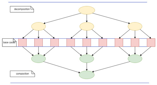
Figure 1.
Task dependency graph of a divide-and-conquer computation with k equal to 3 and with the number of decomposition steps equal to 2.
Parallel divide-and-conquer implementations were extensively studied and they lead to very efficient efficient solutions. If we consider, for example, just the classical sorting algorithms, even these days improvements through different parallelization techniques are proposed [8,9,10,11].
The main goal of this research was to analyze different types of computation that could be designed based on divide-and-conquer pattern, to prove that the divide-and-conquer pattern could be generalized such that to comprise many of the other parallel programming patterns, and to find possible optimizations of it.
The resulting contributions are:
- A new general formal functional specification of the divide-and-conquer pattern;
- Proof that through specific parameters’ instantiation of this general formulation, other classical parallel programming patterns could be obtained;
- A structured analysis of the possible optimizations and execution models of this generalized pattern.
1.1. Paper Outline
The next section gives a brief introduction on parallel programming patterns and skeletons. Section 3 introduces the general formulation proposal of the divide-and-conquer pattern and gives several examples that illustrate different types of divide-and-conquer solutions. The differences between data and task decomposition in the context of the divide-and-conquer pattern are treated in Section 4. Next, in Section 5, the general stages of the divide-and-conquer pattern computation are analyzed along with the possible optimizations that could be obtained by excluding some of them in certain situations; in this context, bottom-up computation is analyzed. Section 6 proves the equivalence between the generalized divide-and-conquer and some of the most common parallel patterns (skeletons). In order to go closer to the implementation level, we analyze in Section 7 different models of execution for divide-and-conquer pattern computation. In Section 8, we analyze the connections with the similar approaches, emphasizing the differences and the advantages.
1.2. Notations
Function application is denoted by a dot , and it has the highest binding power and association from left to right:
- -
- corresponds to classical mathematical notation,
- -
- corresponds to mathematical notation.
Function composition:
- -
- corresponds to classical mathematical notation.
The minimum of two numbers a and b is denoted by , and the maximum by .
The quantification notation that has been used has the following general definition:
where ⊙ is a quantifier (e.g., ∑, ∀, ∃), or a binary associative operator; k is a list of bounded variables; Q is a predicate describing the domain of the bounded variables; and E is an expression. For example, is a computation of the sum of the first 10 square numbers.
Proofs derivations are specified following the styles due to W.F.H. Freijen:
Tuples are denoted using angle brackets—e.g., <>, <>. A tuple function <> is denoted by and is applied to tuples or lists of k length.
The sets are denoted using curly brackets—e.g., .
The lists are denoted using square brackets—e.g., .
Lists operators:
- -
- Concatenation operator——that creates a new list by concatenating two given lists (it could be extended to k lists);
- -
- operator—⊳—that adds an element in front of a given list;
- -
- operator—-⊲—that adds an element at the end of a given list;
- -
- operator—|—is a concatenation of two given lists of the same size (it could be extended to k lists).
- -
- operator—♮—that creates a new list by alternatively taking elements from two given lists of the same size (it could be extended to k lists).
These operators are in the same time constructor operators since they facilitate the construction of new lists from smaller existing lists, and destructor operators since they could be used in order to extract the sublists from a given list.
The length of a list l is given by the function .
Generally, we choose to specify the programs using a functional programming approach only because of the conciseness of this variant. An imperative approach would be different only in the description formulation.
2. Parallel Programming Patterns and Skeletons
The latest developments of the computation systems lead to an increase of the requirements in using parallel computation. In parallel programming, as in programming in general, computation patterns have been defined in order to structure the computation, increase the productivity, and facilitate the analysis and possible implementation improvements. Patterns provide a systematic way of developing the parallel software, and also facilitate a high level of performance and robustness, which are essential in parallel computation. Patterns were generally defined as commonly recurring strategies for dealing with particular problems, and they have been used in architecture [12], natural language learning [13], object-oriented programming [14], and software architecture [15,16].
Classical software engineering approaches based on patterns driven design were proposed for parallel programming, too. Parallel programming patterns lead to better understanding of the parallel computing landscape and to facing challenges of parallel programming developers. In [17], a pattern language was proposed for parallel programming, and this was extended and improved in [18]. Depending on the level of abstraction, patterns could be oriented on design, algorithms or implementations. A structured presentation depending on the patterns level is done in [18]. Four main design spaces were identified:
- Concurrency design space (e.g., Group Tasks; Order Tasks; Data Sharing),
- Algorithm structure design space (e.g., Task Parallelism; Divide and Conquer, Geometric Decomposition; Recursive Data; Pipeline; Event-based Coordination),
- Supporting structures design space (e.g., SPMD–Single Program Multiple Data; Master/Worker; Loop Parallelism; Fork/Join; Shared Data; Shared Queue; Distributed Array),
- Implementation mechanisms design space (e.g., Thread creation/destruction; Process creation/destruction; Synchronization: memory synchronization and fences; barriers; exclusion; Communication: message passing; collective communication).
Algorithm strategy patterns treat how the algorithms are organized, and they are also known as algorithmic skeletons [19,20]. Algorithmic skeletons have been used for the development of various tools providing the application programmer with suitable abstractions. They initially came from the functional programming world, but in time, they have been taken by the other programming paradigms, too.
Skeletons have been treated from two perspectives: semantics and implementation. The semantic view is an abstraction that describes how the skeleton is used as template of an algorithm, and consists of a certain arrangement of tasks and data dependencies. The semantic view is an abstraction that intentionally hides some details, in opposition to the implementation view that provides detailed implementations of a specific skeleton by choosing different low-level approaches on different platforms. The semantic views allow formal approaches that are important for proving correctness, which is an essential issue in a parallel computing setting. Different implementations of a skeleton provide different performances. Through the implementation view, the skeletons differentiate from simple patterns, with skeletons often being used as building blocks for parallel libraries and frameworks such as those presented in [21,22,23,24,25]. These skeleton-based libraries allow a high level of productivity and portability.
If we may reduce the number of patterns (or skeletons) without restraining their power of expressiveness (the power to specify a large class of computation) we may simplify the development of such frameworks.
Divide-and-conquer is one of the most powerful and used parallel computing patterns/skeletons. Early in 1980s and 1990s, there were suggestions in the literature that there is a promising case for considering the divide-and-conquer paradigm as a fundamental design principle with which to guide the design parallel programming [26,27,28,29,30]. Starting from this idea, divide-and-conquer was used even as a base for an experimental parallel programming language—Divacon [31]. The divide-and-conquer skeleton was analyzed using either formal [27,32] or implementation-oriented [33,34] approaches.
3. Divide and Conquer Generalized Pattern
We propose a generalization of the definition of the divide-and-conquer pattern of computation, for which we provide a formal specification.
Definition 1
(General Divide-and-Conquer). A general functional definition of divide-and-conquer computation on inputs of type and outputs of type is defined using the following formulation:
where the parameters have the following meaning:
- The arity list, which defines the number of the subproblems into which the problem is decomposed at each level; for example, if it is equal to , then the first time the decomposing is done into two subproblems, next time, each of these subproblems is decomposed into 3 subproblems, and so forth;
- The decomposition function—δ; this function returns the subdivisions that result through the input decomposition;
- The combine function—θ; this function may use other auxiliary functions in order to combine the solutions of the subproblems;
- The basic functions—α = <> that defines the computation applied for basic cases; we consider that depending on the subproblem’s number, different basic functions could be applied;
- The maximum recursion level (l); this is decremented at each decomposition phase, and if it becomes equal to 0, the decomposition stops even if the arity list is not empty, and the problem is solved using a different method (the alternative computation function β);
- The alternative function—β = <; this function is used when the null recursion level is attained before the termination of the arity list, and before arriving at inputs of type ; it supposes to solve the same problem, but using a different approach (method);
Simplification: The function specification could be simplified in the following cases:
- When the arity-list contains only equal numbers, then the specification could be simplified by replacing the type of the first argument from lists of natural numbers into natural numbers. For example, if the splitting is always done in k subproblems, the function receives a natural number k as the first argument (the decomposition degree).
- The recursion level may be excluded, in which case the alternative specification function () will not be specified, too.If the recursion level is not specified, and the arity list is also replaced with the degree (k) of the decomposition, the recursion depth is implicitly induced by the steps needed to obtain the base cases; it could be computed based on the decomposition function, the degree k, and the given input.
- If the same function is applied for the base cases, then it can be specified as a simple function instead of as a tuple of functions. If the base function () is the identity function, this may be completely excluded from the specification.
- For the function , the same simplification as for the function could be applied, too.
Property 1
(Well-defined). A function is well-defined if:
- -
- If a recursion level l is given, then l is smaller or equal to .
- -
- When the arity-list is empty, the input belongs to , which is a subdomain of the input data for which the computation of the problem could be solved using the α function.
Property 2
(Correctness).
Semantic correctness:If a problem is specified using Hoare triple [35], a function that resolves that problem is correct if for any input from the Input domain that respects the preconditions , the computation terminates and the obtained output respects the postconditions .
In general, this correctness could be proven by induction.
Termination:The termination of the computation of the function is assured if the function is well-defined and the basic function—α, and the alternative function—β (if it is provided) terminate for each possible input derived through splitting from the domain.
Property 3
(Complexity).
Parallel Time Complexity:The parallel time-complexity of the function with the decomposition degree k could be estimated, under the condition of unbounded parallelism, using a recurrent formula as:
where n is the initial size of the problem, and are the sizes of the subproblems, l is the level of recursion, is the time-complexity associated with decomposition operation, and is the time complexity associated with aggregation of the k results.
Sequential Time Complexity:For the sequential time complexity, the operator max in the Equation (5) is replaced with the sum operator ∑.
If the input type is an aggregated type of data and the division is based on data decomposition, then the decomposition function defines a data partition. The sets of the resulted partition may or may not be disjunctive.
Additionally, in general, the number of subproblems into which the problem is decomposed is equal or greater than two (). Still, in the literature, it is also accepted that the decomposition could be done into one or more subproblems [36]. We may accept for this generalized definition that the degree is equal or greater than one (). In [2], the variant with is called “decrease-and-conquer”, and as it is shown in this reference, there are many algorithms that could be solved using this technique. Even if only one subproblem is used, the potential parallelism still exists—the subproblem could be used in several contexts (e.g., Gray code generation—discussed in the next subsection), or when additional computation should be done, and this is independent on the subproblem computation (e.g., scan computation using Ladner and Fischer algorithm—discussed in the next subsection).
3.1. Examples
For the following examples, we will start from functional recursive definitions and from these, instantiations of the general divide-and-conquer pattern are extracted.
3.1.1. Sum
The addition of a given list of numbers could be defined by splitting the list into two parts:
In this case, the decomposition degree is equal to 2, the function is the identity function (and so it is excluded from the arguments’ list), the recursion level is not given and it will be implicitly computed based on the length of the input list, and the function is not given since the decomposition is done until the base case is attained.
If the length of the list is a power of two, then the decomposition list operator should be | (tie operator) that assures decomposition into equally sized lists.
For the addition, we may also define a multi-way divide-and conquer definition as:
or more general using an arity list, and imposing the decomposition into lists of equal lengths using operator | (tie):
The last variant is useful if the number of elements is not a power of a number k and we would like to obtain a balanced decomposition. For example, if the length of the list of given elements is , then the arity list could be equal to , and each time the equal size decomposition operator tie (|) could be used. The arity list should be provided as a parameter since the decomposition into factors could be different (e.g., is another possibility for the same ).
The problem is naturally extended to the more general problem—, where the addition operator is replaced with any associative binary operator.
3.1.2. Merge-Sort
Another popular example is the problem of sorting a list of numbers using the merge-sort method:
where ⋈ (merge operator) is an operator that takes two sorted lists and combine them into a sorted list that contains all the elements from the both input lists. The definition may use the | decomposition operator instead of if it is possible to split into equally sized lists.
For this problem, it could be useful to provide an alternative function definition that specifies a hybrid method, which first decomposes the list using merge-sort and then uses for sorting small size lists:
In this case, the recursion level (l) could stop the recursion before arriving at lists with only one element (the base case), and then apply an alternative sorting method (Quicksort) on the sublists. This is beneficial for the practical parallel execution because the degree of parallelism could be better controlled: when the desired degree of parallelism is achieved, the sorting of the sublists is done sequentially with a very efficient algorithm.
Oppositely, we may increase the degree of parallelization by defining the merging operator (⋈) of two sorted lists also as a divide-and-conquer problem, for which parallel computation is possible:
where the list operator ◇ is defined by:
and the operator ⊙ defined by:
So,
Sequential merge operation could be specified with a recursion based on the and list operators, as it follows:
3.1.3. Reflected Binary Gray Code
Even when the decomposition leads to the computation of only one subproblem, if this is used in several contexts, the potential for parallelization still exists. Such an example is the generation of the Gray code, also named reflected binary code; this is an ordering of the binary numeral system such that two successive values differ in only one bit (binary digit). For example, the classical representation of the decimal value “1” in binary is “001” and of “2” is “010”. In the Gray code, these values are represented as “001” and “011”. In this way, incrementing a value from 1 to 2 requires only one bit to change, instead of two. The recursive definition of the function that computes the binary-reflected Gray code list for n bits is as follows:
By applying fusion to ⇝ and , we obtain :
Thus, can be expressed using the general pattern as:
The subproblem is computed for an argument with a value decremented by 1, but this result is used in two contexts: the first when a 0 is appended in front of the subproblem result, and the second when a 1 is appended in front of the reverse of it, too. Because there are two contexts in which the subproblem is used, the parallelization is still possible: each time two tasks are created. If the parallelization is done in a distributed multiprocessing environment, it is more efficient to locally compute the subproblem instead of communicating the result to the second usage context.
A similar solution could be given for the problem of finding all the subsets with n elements of a given set.
3.1.4. Prefix-Sum
The problem of the prefix sum, or , is used very often in different computation contexts; if we have a list of numbers the the prefix-sum is defined by the following list . Operator + could be replaced with any associative operator.
A simple and direct definition using a recursive strategy is the following:
Another more efficient algorithm for computing the prefix-sum was proposed by Ladner and Fisher [37]. This variant was expressed in a functional recursive way by J. Misra in [38].
The effect of shifting applied to a list is to append the first parameter to the left and discard the rightmost element of the list; thus, .
In this case, we have again only one subproblem used at the decomposition phase, but this subproblem is applied to an argument () that is computed in a divide-and-conquer manner, and the result is used in other computations.
4. Data versus Task Orientation
In a divide and conquer computation, solving each problem (and each subproblem) can be seen as a task, but how these tasks are identified and created depends on the nature of the problem [7]. The decomposition in the divide-and-conquer pattern could be led either by data partition or by data transformation. The decomposition function returns the appropriate values of the subproblem parameters; it is applied on the input data, but it depends if it is something like a data distribution function (generate a data partition) or a function that transforms the input.
Based on this, it is possible to give a classification that identifies these two variants:
- Data oriented divide-and-conquer,
- Task oriented divide-and-conquer.
The most common application of divide-and-conquer is for the problems where the subproblems are identified by decomposing the data input that are of an aggregate type (lists, arrays, sets, trees, etc.). The decomposition starts by decomposing the aggregated data, and then associates the computation with each of the resulted parts of the partition. The examples for , , and belong to this category.
Having as an input a set of functions, which have to be applied on a set of data, it could be treated also as a data-oriented divide-and-conquer since an aggregated list of functions is provided and this could be split as they were any other type of data. Still, in this case, the decomposition is usually done on one single level.
For task oriented divide-and-conquer, the subproblems may be instances of smaller problems (problems with smaller complexity) and the identification of these smaller problems could follow different strategies. Very often they rely on the technique called decrease-and-conquer, as it is the example of the Gray code generation.
Another example is the problem for finding all numbers, which respect a certain property— (e.g., perfect square, prime number, etc.), from a given range—i.e., the range is given and not a list of numbers. The smaller problems are identified by splitting the given range:
for all .
An important category of problems where task oriented divide-and-conquer could be applied is recurrent streams solving:
In this case, the subproblems (the values of the previous elements) could be solved independently, and so based on the definition, we may apply a divide-and conquer pattern. But when solving them, there is an important computation overlapping; the classical way of execution (create a separate task for the computation of each term: ) is not efficient. For optimization, at the execution stage, a memoization technique could be used, which means to store the already computed values into a fast accessible table (map, or hash-table) in order to avoid the re-computation.
When the computation follows a bottom-up strategy, this algorithmic method is encountered with the name dynamic programming. Typically, for this case, the subproblems arise from a recurrence relating a given problem’s solution to solutions of its smaller subproblems. Rather than solving overlapping subproblems again and again, dynamic programming suggests solving each of the smaller subproblems only once and recording the results in a table from which a solution to the original problem can then be obtained. Dynamic programming extends divide and conquer approach with memoization or tabulation technique.
For data driven divide-and-conquer we may identify some special characteristics that may lead to some optimization of the computation. These optimizations are based on the stages of divide-and-conquer computation.
5. Divide-and-Conquer Stages
The application of the divide-and-conquer pattern could be decomposed into three important stages:
- Decomposition (divide)The application of the decomposition function
- Base Computation (base)The application of the basic function
- Composition (combine)The application of the composition function
If the recursion is applied only once, we have:
In most of the cases, the function only has the role of splitting the data input into several subsets; this was the case for the function, but also for .
Still, there are also cases—such as the Ladner and Fisher variant of computation for the prefix sum (Equation (19))—when the decomposition imposes additional operations of the input.
Quicksort is another example where the decomposition function has a much more complex responsibility:
For the cases when the decomposition function just provides a partition of the input, additional optimizations could be provided.
Definition 2
(Simple distribution). If the input data type () is an aggregated data structure, and δ is a decomposing function, then δ is called a simple distribution function ⇔
Theorem 1
(Bottom-up computation). If we have a divide-and-conquer function
applied on an domain formed of lists with the length equal to , and the corresponding decomposing function δ is a simple distribution function, which is formally expressed as:
then we have
where dac_botomup is a function that recursively applies the function θ on subsets of k input elements
Proof of Theorem 1.
Proof by induction
Base case:
Inductive case:
Induction hypothesis is
for any simple distribution , combine function and base function ; and we prove that
We consider
□
- The theorem can be easily extended to divide-and-conquer functions defined with arity lists containing different values and applied on lists of any length.
- Transforming a function into a function is important because facilitates the elimination of the decomposition phase that could be extremely costly for the computation.
- In addition, for the function, reading the data could be combined with their distribution that could increase efficiency, too.
6. Parallel Programming Patterns Equivalence
The functional definition of the skeletons facilitates the reasoning about them, and for the divide-and-conquer generalized pattern we followed the functional definition as well, and so the equivalence between them is done in the same manner.
6.1. Data Oriented Patterns
The equivalences for the patterns Reduce and Scan have been proven in the Section 3.1.
6.1.1. Map
The map pattern defines a computation where a simple operation is applied to all elements of a collection, potentially in parallel.
This definition emphasizes the case of embarrassingly parallel computation [7], in which independent computation is done in parallel. In this case, the recursion depth is equal to 1.
A more general variant could be defined using an arity list () that is constructed based on the length of the input list p.
The list is an arity list that satisfies ; the product of its elements is equal to the length of the list p. The length of the arity list implicitly determines the depth of the recursion.
By introducing the recursion level (l), a generalized variant that offers better control over the parallelization degree, the following can be obtained:
In this case, the simple plays the role of the alternative function. The function is executed sequentially based on the definition:
6.1.2. DMap
The function is a generalization of that applies different functions (given as a list of functions) onto a list of elements. In this case, the input type is , where is a function defined on X ().
Similar generalizations to those done for could be applied to , too.
6.1.3. Stencil
The stencil pattern is a kind of map where each output depends on a “neighborhood” of inputs, and these inputs are a set of fixed offsets relative to the output position. A stencil output is a function of the “neighborhood” elements in an input collection—usually this function is called kernel. Stencil defines the “shape” of the “neighborhood” and since this remains the same, so the data access patterns of stencils are regular.
Being a kind of a , the stencil pattern could be expressed as a function, where the kernel is the base case function. The significant difference is given by the decomposition function () that doesn’t lead to a disjunctive partition—the parts are not disjunctive.
For example, in the case of one-dimensional data structure input, with and the stencil defined by the “neighborhood” at distance 1, the decomposition function and the are defined as follows:
6.1.4. Map-Reduce (Functional Homomorphisms)
Any function that can be defined as a composition of a and a is a homomorphism [39,40,41]. First, a function is applied to all data (map), and then, the results are aggregated through the reduce operation. This can be defined as divide-and-conquer function
, where f is the function applied by on each element of the input, and ⊕ is the associative operator of the function. It could be also consider that the “Apply” stage corresponds to a and the “Combine” stage corresponds to a operation.
6.1.5. MapReduce (Google Pattern)
This pattern is a variation of the map-reduce functional programming pattern. It considers that at the Map phase the results are formed of pairs, where belongs to a domain with comparable values (an order relation is available). The Reduce phase aggregates the values of the pairs that have the same key [42]. This leads to the conclusion that we may consider that there are several reduction operations, one for each key. Additionally, this variant could be expressed with the general divide-and-conquer pattern; considering the decomposition degree equal to 2, the computation could be described as:
where
where
is a merge operator of two sorted lists, that uses
operator ⊗ instead of the simple comparison operator.
The operator ⊗ is defined by:
Based on these, we conclude that
that can be extended to a much higher degree of decomposition, or to a variant based on an arity list.
6.2. Task Oriented Patterns
6.2.1. Task-Farm
Task-farm is a pattern similar to , but oriented on tasks. If in the case of all the functions have the same number of parameters, for the task-farm each task may have different input parameters, in number and types. We have n different tasks that could be independently computed in parallel:
As , the task-farm may be considered a function with all the tasks being functions to be applied for base cases; the base case function is a tuple function that applies all the tasks.
6.2.2. Pipeline
The Pipeline pattern uses ordered stages to process a stream of input values. Pipelines are similar to assembly lines, where each item in the assembly line is constructed in stages. The stages don’t have to have the same type and they are not subproblems of one problem. The parallelism is obtained for this pattern by overlapping the execution of the stages for different data.
Since the parallelism is obtained this way, we may define the computation executed at one step inside the pipeline as a function, with the first argument being the list of functions that correspond to stages, and the second being the data on which these are applied. The function has been proved before to be expressed as a function.
The transfer from one step to another inside the pipeline is a sequential function that could be expressed functionally as:
where:
- -
- is a shift function that inserts an element in the front of list and eliminates the last element—it was defined in Section 3.1;
- -
- p is the input stream of values;
- -
- q is the list of results;
- -
- F is a list of k functions that define the pipeline stages;
- -
- is a mark value that is finally ignored; any function could be applied on it with the results equal to , too;
- -
- l is the list of values that are inside the pipeline; initially, when the function is called first time, this list has to contain values equal to .
7. Models of Execution
Different execution models could be considered for a divide-and-conquer function. They depend on the level of recursion and on the parallelism degree [43]. The following analysis is done for a function of order k with n base cases.
In order to facilitate the description of the models of execution, we will use unit of execution or UE as a generic term for one of a collection of possibly concurrently executing entities, usually either processes or threads. This is acceptable in the early stages of program design, when the distinctions between processes and threads are less important.
Based on the three stages identified for a divide-and conquer computation, we have identified the following classes of divide-and-conquer classes:
- DAC—divide-apply-combine: this is the case of complete divide-and-conquer computation that contains all the stages: decomposition executed on a different number of levels, base case applications, followed by the combination stage. Relevant examples are: and Ladner and Fisher prefix sum.
- AC—apply-combine: this is the case described by the Bottom–Up Theorem, when the decomposition could be omitted because it leads only to a data distribution; the base case is applied on all the values resulted through data distribution, and then they are combined using the number of levels specified. Relevant examples: , .
- A—apply: this is a simplification of a previous case when the combination stage could be omitted, because the combination is reduced to a simple concatenation of the outputs. Relevant examples: .
Since we identified three major classes of divide-and-conquer patterns, the execution models are discussed for each of these three.
In general, two approaches are possible:
- i
- Explicit Execution—for each subproblem, a new task is created and a new UE is created for executing each such task;
- ii
- Implicit Execution—for each subproblem, a new task is created and all these tasks are submitted to a task-pool that is served by a predefined number of UEs.
The specific characteristics with their advantages and disadvantages are identified and analyzed.
7.1. DAC: Divide-Apply-Combine
7.1.1. DAC—Explicit UE Execution
The computation of each subproblem is assigned to a new processing unit (thread, process). These lead to a number of UEs (k is the decomposition degree, and n the number of base cases), which grows very fast with n (the number of base case applications). The needed data are sent to each UEs at the moment of creation. Additionally, any UE excepting the first (the root) should wait for the termination of the UEs spawned by it, and be able to take their results, too.
By specifying the recursion level (l) it is possible to control that UEs creation to a limit equal to .
If k is equal to 2 an efficient approach is to create only one UE at each decomposition: left subproblem is taken by the current UE, and a new UE is created for the right subproblem; this way only n UE are created.
7.1.2. DAC—Implicit UE Execution (Task Pool)
For the computation of each subproblem, a new computational task is created, and these tasks are submitted to an execution task-pool that manages a specified number of UEs.
For this case, the task-pool should be able to manage the synchronization induced by the fact that the computation of each problem depends on the computation of the subproblems into which was decomposed (parent–children dependency). These means that the management of the pool should assure working in fork-join manner, and to put the waiting tasks into a “stand-by” state in order to have an efficient execution. Such an example is Java ForkJoinPool.
7.2. AC: Apply-Combine
When the division stage is equivalent with data partition (disjunctive or not) the execution could exclude the decomposition stage, which is replaced just by data decomposition (as has been proved in Theorem 1).
7.2.1. AC—Explicit UE Execution (Tree-like Execution)
In this case, n UEs are created and each of these will execute in a first stage the corresponding base cases. The second stage of combing is executed in a tree-like fashion. Figure 2 emphasizes the execution for the case when and .
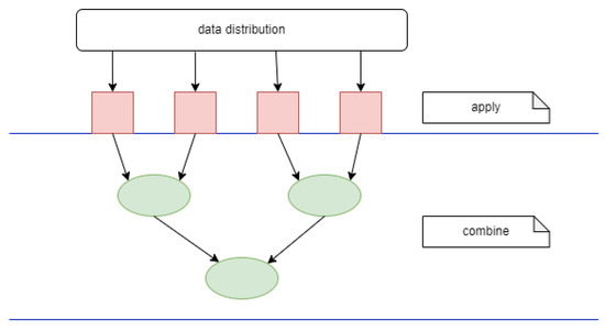
Figure 2.
Tree-like execution for a divide-and-conquer of type AC with k equal to 2 and n equal to 4.
On the distributed memory platforms, the execution has to start with data distribution, through which the processes will receive the needed data.
For the cases when the data partition leads to non-disjunctive data sets, data replication is needed. This is the case of the stencil operations, when the “neighborhood” elements are needed in the computation.
Data distribution could be combined with data reading that in many cases could be executed in parallel: each of the n UE reads the needed data. This approach increases the efficiency very much since reading the input is, in general, a very costly operation.
7.2.2. AC—Implicit UE Execution (Task Pool)
A master UE is needed to manage the creation of the tasks and their submission to the task pool. Initially, it creates n tasks corresponding to each base case and then submits them to the execution pool. After that, the master will create, successively, all the combing tasks depending on the order k and the results of the previous tasks.
The manager is also responsible to attach the needed data to each task and to collect the result.
7.3. A: Apply
When the computation is reduced only to the computation of the base cases, the execution follows a master-workers [18] type of execution.
7.3.1. A—Explicit UE Execution
This execution model leads to the creation of n UEs, one for each of the base cases, and this corresponds to embarrassingly parallel computation [7]. Each UEs could also be responsible for reading the corresponding input data and writing the result.
7.3.2. A—Implicit UE Execution (Master-Workers)
A master UE manages the execution of a number of workers (UEs), which will receive tasks for computing the base cases. The data inputs and outputs are managed by the master.
7.4. Advantages/Disadvantages:
In general, the explicit models have the following advantages and disadvantages:
Advantages:
- -
- Explicit control of the association between computation task and execution unit;
- -
- Communication network (tree) could be mapped explicitly to the interconnection network.
Disadvantages:
- -
- UEs (thread/process) explosion;
- -
- Difficult to manage.
On the other hand the implicit models have their specific advantages and disadvantages:
Advantages:
- -
- The number of UEs is controlled by the execution pool;
- -
- Easy to manage/use.
Disadvantages:
- -
- Implicit control of the association between computation tasks and execution units;
- -
- Communication network (`task-graph’) could not be mapped explicitly to the physical interconnection network; the execution pool is responsible to associate the tasks with the UEs, which on their turn are executed on physical processing elements.
- -
- Specific requirements for the task pool management are imposed.
7.5. Synchronization and Data Management
Divide-and-conquer pattern imposes through the definition synchronization points before each combine operation; in order to apply the combine operations, all the corresponding subproblems should be finalized.
In addition to these implicit synchronization points, the execution model could specify additional ones. These could be related to the necessity of assuring consistency when share data are used.
When data partitioning does not lead to disjunctive data sets and shared memory is used, synchronization is essential in order to assure correctness. A simple solution to avoid this synchronization is possible through data replication, which still may increase space-complexity.
The overall efficiency of a divide-and-conquer algorithm is very dependent upon the efficiency with which the problem can be divided into parts, and the efficiency with which the solutions to the parts can be combined to give the overall solution. Often, large data structures are required to represent the problem data and/or the problem solution. These can lead to the need of a careful analysis of the ways these data structures can be divided and combined. In concrete executions, these imply data communications that have a very important impact over the overall efficiency.
When distributed memory is used, data communication adds an important overhead, that should be optimized through data packaging, data serialization, or by combing reading with data distribution, or/and data aggregation with data writing. Examples of frameworks that treat these problems are those reported in [44,45].
For implicit execution, several optimizations have been proposed [46,47]. Optimizations based on techniques such as "work-stealing" were proposed, and they fit very well for of divide-and-conquer problems with a high degree of imbalance among the generated subproblems and/or a deep level of recurrence. Using the proposed generalized formulation the level of recurrence is better controlled, and this could provide better adaptation to a much larger class of thread pool executors.
8. Discussion
We provided a more general definition of the divide-and-conquer pattern that includes an arity list for different decomposition degrees, a level of recursion, and also an alternative solution for the cases that are not trivial, but could be solved sequentially in an efficient way.
Very often, the number of the subproblems is equal to 2; the proposed generalized variant not only accepts a decomposition in more than 2 problems, but also includes the variant when at each level of decomposition the arity could be different. This brings the advantage of eliminating some constraints regarding the size of the problem; if, for example, in a simple search problem the size of the collection (n) is not a power of two we cannot split the collection always into two equal parts, but still we may use the decomposition of n in factors, and so, we allow the possibility to always split into subcollections of equal sizes.
By introducing the parameter for the level of recursion, we allow applying a hybrid solution of the problem in hand: a composition of a solution based on divide-and-conquer (until a certain level) and another solution for the problems of a certain size (complexity). This could be useful from the complexity point of view, since for a sequential execution the recursion involved by the divide-and-conquer could bring additional costs. A detailed explanation was given for the algorithm.
In addition, the level of recursion provides the possibility to control the degree of parallelization: a parallel model of execution is used only until the level of recursion is greater than zero. This doesn’t exclude the possibility of using the same decomposition for the rest of the computation, but using classical sequential execution of the divide-and-conquer computation (in this case, the function is defined similarly with the initial , but without a level of recursion parameter). On the other hand, the alternative computation provided through the function may provide a non-recursive solution that has a more efficient implementation. For example, for the addition example, the function can be the simple iterative addition function, for which the execution time is much smaller than for one implemented based on recursion.
Starting from this generalized specification of the pattern, we proved that it can be instantiated such that to obtained other classical parallel programming patterns as: , , , , , and . For pattern a specification is provided based on a recursive function and a (which is an instance of ) composition.
Having a generalized specification of a pattern, from which we may derive through specialization other patterns, is useful either from formal semantic point of view, since it allows reasoning for a wide class of computations, but also from an implementation point of view, since it allows generic implementations.
Going closer to the implementation level, we have analyzed several models of executions depending on the class of the divide-and-conquer computation and the type of parallelization: with explicit or implicit association between the tasks and the unit of executions (thread or processes).
The idea of providing a generalized formulation of the divide-and-conquer pattern came from our experience of implementing a parallel programming framework (JPLF) [48] based on a variant of this pattern that uses PowerList and Plist data structures introduced by J. Misra [38], and so oriented on data decomposition. The JPLF framework offers the possibility to develop efficient implementations based on some templates that facilitate a simple and robust implementation. Using it, we proved that this can lead to efficient implementations on shared and distributed memory platforms of many divide-and-conquer algorithms [45,48,49,50]. The templates based on PowerList allow decompositions of degree two (decomposition into two subproblems), while the variants based on PList allow decomposition with different arities [51].
Starting from the experience of developing this framework, we intend to create a more general one that relies on this new general functional specification of the pattern as a base model and that follows the framework architecture proposed in [52], which emphasizes the necessity of having all the following components: Model, Executors, DataManager, UserInteracter, GranularityBalancer, and MetricsAnalyser.
The future work plans also include the implementation and evaluation in terms of various execution models of different divide-and-conquer algorithms in order to show the effectiveness of the proposed generalized approach.
Funding
This research was funded partially funded by the Robert Bosch GmbH through a contract that sustains the research in the domain of Big Data Analytics and High performance Computing at the Faculty of Mathematics and Computer Science, “Babes-Bolyai” University.
Data Availability Statement
Not applicable.
Conflicts of Interest
The authors declare no conflict of interest.
Abbreviations
The following abbreviations are used in this manuscript:
| DAC | divide-apply-combine |
| AC | apply-combine |
| A | apply |
References
- Cormen, T.H.; Leiserson, C.E.; Rivest, R.L. Introduction to Algorithms, 3rd ed.; MIT Press: Cambridge, MA, USA, 2009. [Google Scholar]
- Levitin, A.V. Introduction to the Design and Analysis of Algorithms, 3rd ed.; Addison Wesley: Boston, MA, USA, 2002. [Google Scholar]
- Hoare, C.A.R. Algorithm 64: Quicksort. Commun. ACM 1961, 4, 321. [Google Scholar] [CrossRef]
- Aung, M.N.; Phyo, Y.; Do, C.M.; Ogata, K. A Divide and Conquer Approach to Eventual Model Checking. Mathematics 2021, 9, 368. [Google Scholar] [CrossRef]
- Wu, J.; Li, Y.; Shi, L.; Yang, L.; Niu, X.; Zhang, W. ReRec: A Divide-and-Conquer Approach to Recommendation Based on Repeat Purchase Behaviors of Users in Community E-Commerce. Mathematics 2022, 10, 208. [Google Scholar] [CrossRef]
- Delgado-Gómez, D.; González-Landero, F.; Montes-Botella, C.; Sujar, A.; Bayona, S.; Martino, L. Improving the Teaching of Hypothesis Testing Using a Divide-and-Conquer Strategy and Content Exposure Control in a Gamified Environment. Mathematics 2020, 8, 2244. [Google Scholar] [CrossRef]
- Grama, A.; Gupta, A.; Vipin, G.; Kumar, K. Introduction to Parallel Computing, 2nd ed.; Addison-Wesley: Boston, MA, USA, 2003. [Google Scholar]
- Al-Adwan, A.; Zaghloul, R.; Mahafzah, B.A.; Sharieh, A. Parallel quicksort algorithm on OTIS hyper hexa-cell optoelectronic architecture. J. Parallel Distrib. Comput. 2020, 141, 61–73. [Google Scholar] [CrossRef]
- Tsigas, P.; Zhang, Y. A simple, fast parallel implementation of Quicksort and its performance evaluation on SUN Enterprise 10000. In Proceedings of the Eleventh Euromicro Conference on Parallel, Distributed and Network-Based Processing, Genova, Italy, 5–7 February 2003; pp. 372–381. [Google Scholar] [CrossRef]
- Ganapathi, P.; Chowdhury, R. Parallel Divide-and-Conquer Algorithms for Bubble Sort, Selection Sort and Insertion Sort. Comput. J. 2021, 65, 2709–2719. [Google Scholar] [CrossRef]
- Langr, D.; Schovánková, K. CPP11sort: A parallel quicksort based on C++ threading. Concurr. Comput. Pract. Exp. 2022, 34, e6606. [Google Scholar] [CrossRef]
- Alexander, C. A Pattern Language: Towns, Buildings, Construction; Oxford University Press: Oxford, UK, 1977. [Google Scholar]
- Kamiya, T. Japanese Sentence Patterns for Effective Communication; Kodansha International: Tokyo, Japan, 2012. [Google Scholar]
- Gamma, E.; Helm, R.; Johnson, R.; Vlissides, J. Design Patterns: Elements of Reusable Object-Oriented Software; Addison-Wesley Longman Publishing Co., Inc.: Boston, MA, USA, 1995. [Google Scholar]
- Schmidt, D.C.; Fayad, M.; Johnson, R.E. Software Patterns. Commun. ACM 1996, 39, 37–39. [Google Scholar] [CrossRef]
- Buschmann, F.; Meunier, R.; Rohnert, H.; Sommerlad, P.; Stal, M. Pattern-Oriented Software Architecture; Wiley: Hoboken, NJ, USA, 1996. [Google Scholar]
- Massingill, B.L.; Mattson, T.G.; Sanders, B.A. A Pattern Language for Parallel Application Programs. In Proceedings of the Euro-Par 2000 Parallel Processing, Munich, Germany, 29 August–1 September 2000; Bode, A., Ludwig, T., Karl, W., Wismüller, R., Eds.; Springer: Berlin/Heidelberg, Germany, 2000; pp. 678–681. [Google Scholar]
- Mattson, T.; Sanders, B.; Massingill, B. Patterns for Parallel Programming, 1st ed.; Addison-Wesley Professional: Boston, MA, USA, 2004. [Google Scholar]
- Cole, M. Algorithmic Skeletons: Structured Management of Parallel Computation; MIT Press: Cambridge, MA, USA, 1991. [Google Scholar]
- Aldinucci, M.; Danelutto, M. Skeleton-based parallel programming: Functional and parallel semantics in a single shot. Comput. Lang. Syst. Struct. 2007, 33, 179–192. [Google Scholar] [CrossRef]
- Ciechanowicz, P.; Poldner, M.; Kuchen, H. The Münster Skeleton Library Muesli: A Comprehensive Overview; Working Papers No. 7; ERCIS-European Research Center for Information Systems: Münster, Germany, 2009. [Google Scholar]
- Ernstsson, A.; Li, L.; Kessler, C. SkePU 2: Flexible and Type-Safe Skeleton Programming for Heterogeneous Parallel Systems. Int. J. Parallel Programing 2018, 46, 62–80. [Google Scholar] [CrossRef]
- Aldinucci, M.; Danelutto, M.; Kilpatrick, P.; Torquati, M. Fastflow: High-Level and Efficient Streaming on Multicore. In Programming Multi-Core and Many-Core Computing Systems; Wiley: Hoboken, NJ, USA, 2017; Chapter 13. [Google Scholar] [CrossRef]
- Emoto, K.; Hu, Z.; Kakehi, K.; Takeichi, M. A Compositional Framework for Developing Parallel Programs on Two-Dimensional Arrays. Int. J. Parallel Program. 2007, 35, 615–658. [Google Scholar] [CrossRef]
- Karasawa, Y.; Iwasaki, H. A Parallel Skeleton Library for Multi-core Clusters. In Proceedings of the 2009 International Conference on Parallel Processing, Vienna, Austria, 22–25 September 2009; pp. 84–91. [Google Scholar] [CrossRef]
- Horowitz, E.; Zorat, A. Divide-and-Conquer for Parallel Processing. IEEE Trans. Comput. 1983, 32, 582–585. [Google Scholar] [CrossRef]
- Mou, Z.G.; Hudak, P. An algebraic model for divide-and-conquer and its parallelism. J. Supercomput. 1988, 2, 257–278. [Google Scholar] [CrossRef][Green Version]
- Axford, T. The Divide-and-Conquer Paradigm as a Basis for Parallel Language Design. In Advances in Parallel Algorithms; John Wiley & Sons, Inc.: Hoboken, NJ, USA, 1992; pp. 26–65. [Google Scholar]
- Cole, M. On dividing and conquering independently. In Proceedings of the Euro-Par’97 Parallel Processing, Passau, Germany, 26–29 August 1997; Lengauer, C., Griebl, M., Gorlatch, S., Eds.; Springer: Berlin/Heidelberg, Germany, 1997; pp. 634–637. [Google Scholar]
- Amor, M.; Argüello, F.; López, J.; Plata, O.; Zapata, E.L. A Data-Parallel Formulation for Divide and Conquer Algorithms. Comput. J. 2001, 44, 303–320. [Google Scholar] [CrossRef]
- Mou, Z. Divacon: A parallel language for scientific computing based on divide-and-conquer. In Proceedings of the Third Symposium on the Frontiers of Massively Parallel Computation, College Park, MD, USA, 8–10 October 1990; pp. 451–461. [Google Scholar] [CrossRef]
- Gorlatch, S.; Lengauer, C. Parallelization of Divide-and-Conquer in the Bird-Meertens Formalism. Form. Asp. Comput. 1995, 7, 663–682. [Google Scholar] [CrossRef]
- Poldner, M.; Kuchen, H. Skeletons for Divide and Conquer Algorithms. In Proceedings of the IASTED International Conference on Parallel and Distributed Computing and Networks, PDCN’08, Innsbruck, Austria, 12–14 February 2008; ACTA Press: Anaheim, CA, USA, 2008; pp. 181–188. [Google Scholar]
- Danelutto, M.; Matteis, T.D.; Mencagli, G.; Torquati, M. A divide-and-conquer parallel pattern implementation for multicores. In Proceedings of the 3rd International Workshop on Software Engineering for Parallel Systems, Grenoble, France, 24–26 August 2016. [Google Scholar]
- Hoare, C.A.R. An Axiomatic Basis for Computer Programming. Commun. ACM 1969, 12, 576–580. [Google Scholar] [CrossRef]
- Goodrich, M.; Tamassia, R. Algorithm Design: Foundation, Analysis and Internet Examples; Wiley India Pvt. Limited: New Delhi, India, 2006. [Google Scholar]
- Ladner, R.E.; Fischer, M.J. Parallel Prefix Computation. J. ACM 1980, 27, 831–838. [Google Scholar] [CrossRef]
- Misra, J. Powerlist: A Structure for Parallel Recursion. ACM Trans. Program. Lang. Syst. 1994, 16, 1737–1767. [Google Scholar] [CrossRef]
- Gorlatch, S. Extracting and implementing list homomorphisms in parallel program development. Sci. Comput. Program. 1999, 33, 1–27. [Google Scholar] [CrossRef]
- Hu, Z.; Iwasaki, H.; Takeichi, M. Construction of list homomorphisms by tupling and fusion. In Proceedings of the Mathematical Foundations of Computer Science 1996, Craców, Poland, 2–6 September 1996; Penczek, W., Szałas, A., Eds.; Springer: Berlin/Heidelberg, Germany, 1996; pp. 407–418. [Google Scholar]
- Cole, M. Parallel Programming with List homomosrphisms. Parallel Process. Lett. 1995, 5, 191–203. [Google Scholar] [CrossRef]
- Dean, J.; Ghemawat, S. MapReduce: Simplified Data Processing on Large Clusters. Commun. ACM 2008, 51, 107–113. [Google Scholar] [CrossRef]
- Mattson, T.G.; Sanders, B.A.; Massingill, B.L. A Pattern Language for Parallel Programming; Addison Wesley Software Patterns Series; Addison Wesley: Boston, MA, USA, 2004. [Google Scholar]
- Martínez, M.A.; Fraguela, B.B.; Cabaleiro, J.C. A highly optimized skeleton for unbalanced and deep divide-and-conquer algorithms on multi-core clusters. J. Supercomput. 2022, 78, 10434–10454. [Google Scholar] [CrossRef]
- Niculescu, V.; Bufnea, D.; Sterca, A. MPI Scaling Up for Powerlist Based Parallel Programs. In Proceedings of the 2019 27th Euromicro International Conference on Parallel, Distributed and Network-Based Processing (PDP), Pavia, Italy, 13–15 February 2019; pp. 199–204. [Google Scholar] [CrossRef]
- González, C.H.; Fraguela, B.B. A general and efficient divide-and-conquer algorithm framework for multi-core clusters. Clust. Comput. 2017, 20, 2605–2626. [Google Scholar] [CrossRef]
- Martínez, M.A.; Fraguela, B.B.; Cabaleiro, J.C. A Parallel Skeleton for Divide-and-conquer Unbalanced and Deep Problems. Int. J. Parallel Program. 2021, 49, 820–845. [Google Scholar] [CrossRef]
- Niculescu, V.; Loulergue, F.; Bufnea, D.; Sterca, A. A Java Framework for High Level Parallel Programming Using Powerlists. In Proceedings of the 2017 18th International Conference on Parallel and Distributed Computing, Applications and Technologies (PDCAT), Taipei, Taiwan, 18–20 December 2017; pp. 255–262. [Google Scholar] [CrossRef]
- Niculescu, V.; Loulergue, F.; Bufnea, D.; Sterca, A. Pattern-driven Design of a Multiparadigm Parallel Programming Framework. In Proceedings of the 15th International Conference on Evaluation of Novel Approaches to Software Engineering—ENASE, INSTICC, Prague, Czech Republic, 5–6 May 2020; SciTePress: Setúbal, Portugal, 2020; pp. 50–61. [Google Scholar] [CrossRef]
- Niculescu, V.; Loulergue, F. Transforming powerlist-based divide-and-conquer programs for an improved execution model. J. Supercomput. 2020, 76, 5016–5037. [Google Scholar] [CrossRef]
- Niculescu, V.; Bufnea, D.; Sterca, A. PList-based Divide and Conquer Parallel Programming. J. Commun. Softw. Syst. 2020, 16, 197–206. [Google Scholar] [CrossRef]
- Niculescu, V.; Sterca, A.; Loulergue, F. Reflections on the Design of Parallel Programming Frameworks. In Proceedings of the Evaluation of Novel Approaches to Software Engineering, Virtual, 26–27 April 2021; Ali, R., Kaindl, H., Maciaszek, L.A., Eds.; Springer International Publishing: Cham, Switzerland, 2021; pp. 154–181. [Google Scholar] [CrossRef]


Publisher’s Note: MDPI stays neutral with regard to jurisdictional claims in published maps and institutional affiliations. |
© 2022 by the author. Licensee MDPI, Basel, Switzerland. This article is an open access article distributed under the terms and conditions of the Creative Commons Attribution (CC BY) license (https://creativecommons.org/licenses/by/4.0/).