Article

Open-Source Computational Photonics with Auto Differentiable Topology Optimization

School of Electronic Engineering and Computer Science, Queen Mary University of London, London E1 4NS, UK
*
Author to whom correspondence should be addressed.
Current address: Department of Mathematics, Imperial College London, London SW7 2AZ, UK.
Mathematics 2022, 10(20), 3912; https://doi.org/10.3390/math10203912
Submission received: 27 July 2022 / Revised: 16 October 2022 / Accepted: 18 October 2022 / Published: 21 October 2022

Abstract

:
In recent years, technological advances in nanofabrication have opened up new applications in the field of nanophotonics. To engineer and develop novel functionalities, rigorous and efficient numerical methods are required. In parallel, tremendous advances in algorithmic differentiation, in part pushed by the intensive development of machine learning and artificial intelligence, has made possible large-scale optimization of devices with a few extra modifications of the underlying code. We present here our development of three different software libraries for solving Maxwell’s equations in various contexts: a finite element code with a high-level interface for problems commonly encountered in photonics, an implementation of the Fourier modal method for multilayered bi-periodic metasurfaces and a plane wave expansion method for the calculation of band diagrams in two-dimensional photonic crystals. All of them are endowed with automatic differentiation capabilities and we present typical inverse design examples.

1. Introduction

Controlling the flow of light with sub-wavelength photonic devices can be realized by taking advantage of the huge number of degrees of freedom in such systems. This versatility paves the way for the development of highly efficient and compact integrated devices, promising a number of improvements in the growing fields of photonics and optoelectronics. Historically, engineers and researchers have relied on trial-and-error approaches, where a small set of key parameters is tuned to achieve an acceptable level of matching with a predefined figure of merit required by the application. This intuition-based method has helped to develop a diverse and extensively used collection of designs, taking advantage of photonic resonances, dispersion engineering, waveguiding or antenna radiation principles, and enabling an increasingly finer control of light across the electromagnetic spectrum.
On the other hand, accurate manipulation of light can be supported by so-called inverse design, where the process is automated by an optimization algorithm to attain specific device performances under prescribed constraints. In the past two decades, gradient-based topology optimization (TO) [1] has become a widely used tool in computational electromagnetism [2] and has allowed the inverse design of a broad range of devices such as invisibility cloaks [3,4], illusion devices [5], photonic crystals [6,7], metamaterials [8,9], and metasurfaces [10,11,12], to name a few. In essence, density-based TO is an inverse design procedure that can produce highly optimized structures to obtain a prescribed objective. One of its main advantages is to offer unparalleled design freedom since the material distribution is updated locally (at the pixel or voxel level) inside the domain of interest. On the other hand, fabrication constraints often limit this flexibility and several auxiliary tools can be included to tackle those issues [13], for instance, imposing minimal length scales or ensuring the connectivity of the resulting layout. At the heart of this method is computing the gradient of the objective function with respect to the design parameters. Since the number of degrees of freedom is usually prohibitively high to obtain the gradient using naive finite differences, adjoint sensitivity analysis [14] is an indispensable part of all inverse design algorithms. This method can be often implemented straightforwardly and often referred to as the backward simulation, typically derived analytically and hard coded. However, there are instances where the electromagnetic simulation makes the link between the input parameters and the objective function complex, and it would, therefore, be tedious to develop the approach reliably in such a non-trivial context.
In computational science, automatic differentiation (AD) is the application of the adjoint method to arbitrary computational graphs. At the core of an AD programming framework is gradient-aware elementary functions, which allow the software developer to implement only the forward simulation and compose the elementary building blocks to produce more complex code with gradient support.
Here we first report the development of software libraries with automatic differentiation capabilities: a finite element method (FEM)-based code for 2D scattering problems, an implementation of the Fourier modal method (FMM) for stacked bi-periodic structures, and a plane wave expansion method (PWEM) to compute the eigenmodes of 2D photonic crystals. After describing the methods and the automatic differentiation and topology optimization tools, we give examples of application for each: the design of supperscattering structures with the FEM, of a metasurface optimized to transmit maximally in a given diffraction order with the FMM, and maximization of bandgap and dispersion engineering in dielectric photonic crystals using the PWEM.

2. Materials and Methods

Our starting point common to all methods are Maxwell’s equations in the time-harmonic regime with a convention in exp ( i ω t ) assumed throughout:
curl × H = i ω ε 0 ε E
curl × E = i ω μ 0 μ H

2.1. Finite Element Method

We will take as an example a scattering of a plane wave by an infinitely long object denoted Ω s embedded in a background with permittivity ε b and permeability μ b . The problem is assumed to be independent of z (i.e., a two-dimensional simulation) and we only consider z-anisotropic materials, so that the permittivity ε and permeability μ are written as [15]:
ε = ε x x ε a 0 ε a ε y y 0 0 0 ε z z , μ = μ x x μ a 0 μ a μ y y 0 0 0 μ z z .
We consider a plane wave of wavelength λ 0 incident in the x y plane so the two polarizations decouple and Maxwell’s equations can be combined into the following scalar propagation equation:
M ξ , χ ( u ) = · ξ u + k 0 2 χ u = 0 ,
where k 0 = 2 π / λ 0 = ω / c , c is the speed of light in vacuum, u = H z , ξ = ε T / det ε , χ = μ z z for TE polarization, and u = E z , ξ = μ T / det μ , χ = ε z z for TM polarization. Here μ and ε denote the left upper 2 × 2 matrices extracted from μ and ε , T matrix transposition and complex conjugation. Denoting u 0 = exp ( j k · r ) the impinging plane wave, the diffracted field u s = u u 0 must satisfy an outgoing waves condition. We can then recast the scattering problem (4) into a radiation problem:
M ξ , χ ( u s ) = M ξ ξ b , χ χ b ( u 0 ) = S .
We note that the source is localized inside the object since by definition M ξ b , χ b ( u 0 ) = 0 . Perfectly matched layers (PMLs, [16,17]) with constant stretching coefficient are used to truncate the infinite background. The weak form is obtained by multiplying Equation (4) by the complex conjugate of a test function v and integrating by part:
R ξ , χ ( u , v ) = Ω d r ξ u v + Ω d r   χ u v + Ω ds ( ξ u ) v .
The surface term is set to zero by setting homogeneous Neumann boundary conditions ( ξ u ) · n = 0 on the outer boundaries of the PMLs. The solution u of the weak formulation can, therefore, be defined as the element of the space L 2 ( curl , Ω ) the Hilbert space of square-integrable functions with a square-integrable curl on Ω such that:
R ξ , χ ( u , v ) = 0 , v L 2 ( curl , Ω )
The numerical results are obtained using open-source libraries with bindings for the python programming language using a custom code gyptis [18]. The mesh generation is obtained by gmsh [19] and the resolution of Equation (7) is performed with the finite element method (FEM) library fenics [20] using second-order Lagrange basis functions.

2.2. Fourier Modal Method

The Fourier modal method (FMM), also known as rigorous coupled wave analysis (RCWA), is particularly suited for modelling a specific type of periodic structure made up of layers that are invariant in the direction of periodicity. The key idea is to expand the electromagnetic fields within each layer into eigenmodes represented using a Fourier basis in the plane of periodicity. Our implementation considers non-magnetic, possibly z-anisotropic materials (see Equation (3)) and follows closely the derivation from references [21,22]. The structure is assumed to be periodic in the x y -plane with lattice vectors l 1 and l 2 . Each layer is normal to the z-axis and indexed by i with thickness d i and extending from z = z i to z = z i + d i . The semi-infinite substrate ( z < 0 ) and superstrate ( z > Σ i = 1 M 1 d i ) are denoted layer 0 and M, respectively. The reciprocal lattice is defined by the columns of L k = 2 π L r T where L r is the matrix whose columns are l 1 and l 2 and T denotes the transpose of the inverse matrix. The structure is illuminated by a plane wave from the superstrate with incident wavevector k inc with in-plane component k .
The rescaled magnetic field H ˜ = μ 0 / ε 0 H is expanded as:
H ˜ ( r , z ) = G H G ( z ) e i ( k + G ) · r ,
with G = n L k , 1 + m L k , 2 a reciprocal lattice vector and r the in-plane component of the position vector. In practice, this sum must be truncated to retain n h terms to perform a numerical simulation. Defining the Fourier transform:
ε ^ G = 1 L r Ω ε ( r ) e i G · r d r
where Ω denotes one unit cell of the lattice, one can form block Toepliz matrices ε ^ m n = ε ^ G m G n for each component of ε . We denote by h ( z ) the vector H G 1 ( z ) , H G 2 ( z ) , T , and similarly for e ( z ) . The Fourier coefficients d x and d y of the displacement field D are related to the electric field by:
d y ( z ) d x ( z ) = E e y ( z ) e x ( z )
The calculation of matrix E is a subtle matter since one needs to take into account discontinuities in both ε and E [23]. The earliest FMM formulations [24] simply used Laurent’s rule directly, i.e.,:
E = ε ^ x x ε ^ x y ε ^ y x ε ^ y y .
Later, Li introduced the proper Fourier factorization rules [25] and observed an improved convergence of the method. Whilst this is straightforwardly implemented for 1D gratings, for bi-periodic structures, one needs to find a normal field to decompose the electric field in its normal and tangential components at material interfaces [26,27]. In the rest of this subsection, we will assume for simplicity an isotropic permittivity, but the method can be generalized to tensorial ε [28]. Assuming there exists a smooth (possibly complex) field t tangent at all material interfaces, we can apply a change of coordinates from Cartesian to the local basis defined by t and then get in real space:
D y D x = T ε   η 1 T 1 E y E x , T = t y t x t x t y ,
with η 1 = ε . Note that there are several ways to translate Equation (10) in Fourier space. In our implementation, we first expand Equation (10):
D y D x = ε     ε Δ     Δ P y y P y x P x y P x x E y E x ,
with Δ = ε η 1 and
P y y P y x P x y P x x = 1 t 2 t y 2 t x t y t x t y t x 2 ,
and so in the reciprocal space, we have:
E = ε ^     ε ^ Δ ^     Δ ^ P ^ y y P ^ y x P ^ x y P ^ x x .
After Fourier transforming Equations (1) and (2) and eliminating the z components, one gets the matrix equations:
k 0 2 I K h x ( z ) h y ( z ) = i k 0 e y ( z ) e x ( z )
k 0 2 E K e y ( z ) e x ( z ) = i k 0 h x ( z ) h y ( z )
with
K = k ^ y ε ^ z 1 k ^ y k ^ y ε ^ z 1 k ^ x k ^ x ε ^ z 1 k ^ y k ^ x ε ^ z 1 k ^ x , K = k ^ x k ^ x k ^ x k ^ y k ^ y k ^ x k ^ y k ^ y ,
where I is the identity matrix of size 2 n h × 2 n h and f = f / z , and k ^ ν , ν { x , y } , are diagonal matrices with entries k ν + G 1 ν , k ν + G 2 ν , .
The next step is to compute the modes of a given layer, assuming the following ansatz for the magnetic field eigenmode:
H ( z ) = G ϕ G , x x + ϕ G , y y k x + G x ϕ G , x + k y + G y ϕ G , y q z e i ( k + G ) · r + i q z
where x , y , and z are the unit vectors of our Cartesian coordinate system and ϕ ν = ϕ G 1 , ν , ϕ G 2 , ν , T , ν { x , y } are column vectors containing expansion coefficients. We thus have h ( z ) = ϕ x x + ϕ y y q 1 k ^ x ϕ x + k ^ y ϕ y z e i q z . Using Equations (13) and (14), eliminating the electric field and remarking that K K = 0 , we get the following eigenvalue problem:
M Φ = E k 0 2 K K Φ = Q 2 Φ , Φ = ϕ x ϕ y
where Q 2 is the diagonal matrix whose diagonal elements are the eigenvalues q n 2 . The columns of the square matrix Φ are ϕ x , n , ϕ y , n T , the Fourier coefficients of the eigenmodes. Once this crucial and most computationally intensive step has been achieved, the field inside each layer can be recovered as a linear combination of propagating and counter-propagating waves:
h x ( z ) h y ( z ) = n ϕ x , n ϕ y , n a n e i q n z + b n e i q n d i z .
The S-matrix algorithm [21,29] is then used starting from the incident medium to recursively find the S-matrix of each layer and form the total S-matrix. Finally, relevant electromagnetic quantities of interest, such as diffraction efficiencies in transmission and reflection for each order can be retrieved by computing the power flux through the outermost layers, and this is vastly more efficient in Fourier space [22].

2.3. Plane Wave Expansion Method

We will limit our discussion to two-dimensional bi-periodic media with possibly z-anisotropic materials in ε and μ but we consider for simplicity non-dispersive properties. As in Section 2.1, the field decouples and we can expand the z components as:
u ( r ) = G u G   e i ( k + G ) · r ,
After Fourier transforming Maxwell’s equations and recombining the relevant z component of the fields, we get the following generalized eigenproblem:
Q T   ε ^ 1   Q   Φ = k 0 2   χ z z   Φ
where Q = k ^ y , k ^ x T and Φ = u G 1 , u G 2 , T are column vectors containing expansion coefficients.
To further speed up the band diagram computation, we employ a reduced Bloch mode expansion (RBME) [30], only solving Equation (17) at symmetry points of the first Brillouin zone and performing a second expansion using those chosen modes as a basis set. This technique maintains accuracy while reducing the computation time by up to two orders of magnitude.

2.4. Automatic Differentiation

For more than fifty years, automatic differentiation [31,32] (AD) has been applied in a broad range of applications, and its implementation in various programming languages has been boosted by the recent advent of machine learning [33]. Our goal here is to give a brief introduction to this field and how it will be applied to the results of this study. AD may be described as a computer paradigm, therefore, closely connected to a program or a particular family of techniques that compute derivatives via accumulation of values throughout code execution to output numerical derivative evaluations. In brief, it performs an interpretation of a given computer program as a computational graph and propagates derivatives using the chain rule of differential calculus. As soon as this graph is built, the gradient computation turns into a series of fundamental building-block operations.
We assume that the solution vector u we want to compute is parametrized by a vector of parameters p of size M and defined implicitly through an operator F as:
F ( u , p ) = 0
Finally, let G be a functional of interest of dimension N, representing the quantity to be optimized: for instance, the quality of a design to be maximized, or the error between a target and computations to be minimized.
To obtain the derivative of the functional with respect to the design variables, several approaches can be used. A simple idea is to use an approximation using finite differences:
d G d p i G ( p + h e i ) G ( p ) h
where e i is the vector with 0 in all entries except for 1 in the ith entry. However, in addition to the uncertainty on the choice of the parameter h giving potentially numerical inaccuracy, this approach is prohibitively computationally demanding for large M and/or N.
Explicitly, the gradient can be computed by applying the chain rule:
d G d p = G p + G u d u d p .
Taking the total derivative of Equation (18) we obtain the tangent linear equation:
F ( u , p ) u d u d p = F ( u , p ) p .
This is similar to forward mode differentiation and scales linearly with the number of inputs M. However, in typical topology optimization problems, the number of input parameters is generally much larger than the number of output objectives, so this technique is rather inefficient.
Assuming the tangent linear system is invertible, we can rewrite the Jacobian as:
d u d p = F ( u , p ) u 1 F ( u , p ) p .
After substituting this value in (20) and taking the adjoint (Hermitian transpose, denoted by †) we get:
d G d p = G p F ( u , p ) p F ( u , p ) u G u .
Defining the adjoint variable λ as:
λ = F ( u , p ) u G u
we obtain the adjoint equation
F ( u , p ) u λ = G u .
For a given functional (output), the adjoint solution can be used to easily compute the gradient with respect to any parameter. Therefore, solving the adjoint system is extremely efficient when M N . This approach is closely linked to reverse-mode differentiation in AD or backpropagation in the context of neural networks since the flow of information in the equation system is reversed.
For the FEM simulations, we use the library dolfin-adjoint [34], extending fenics with automatic differentiation through the resolution of the adjoint equation. We implemented the FMM and PWEM in python with various numerical backends for core linear algebra operations and array manipulation, with the ability to switch between them: numpy [35], scipy [36], jax [37], autograd [38], and pytorch [39,40]. The latest two libraries have built-in support for automatic differentiation.

2.5. Topology Optimization

We consider a design domain Ω des in which the material distribution is parametrized by a continuous scalar density function p [ 0 , 1 ] . A filtered density p ˜ is used to avoid smaller features and pathological “chessboard” patterns. We use two methods: the first one consists in solving the following Helmholtz equation [41] with homogeneous Neumann boundary conditions on Ω des :
R f 2 2 p ˜ + p ˜ = p ,
with R f being a real positive parameter characterizing the filter radius. This partial differential equation (PDE) based filter is more suited and easily implemented using the FEM. For other numerical methods, we use a Gaussian filter f ( r ) = 1 A exp ( | r | 2 / R f 2 ) , with the normalization A chosen such that Ω des f ( r ) = 1 . The filtered density in this case is obtained by a convolution:
p ˜ ( r ) = p f = Ω des p ( r ) f ( r r ) d r
A threshold projection is then used to progressively obtain a binary design consisting of two materials only [42]:
p ^ ( p ˜ ) = tanh β ν + tanh β ( p ˜ ν ) tanh β ν + tanh β ( 1 ν ) ,
where the level of projection ν = 1 / 2 and β is a real positive parameter and is increased during the course of the optimization. Finally, the permittivity inside the design region is defined using the solid isotropic material with penalization (SIMP) method [43] as
ε ( p ^ ) = ( ε max ε min )   p ^ + ε min ,
The gradient-based optimization is initialized with a density p 0 and performed for 40 iterations or until convergence on the objective or design variables. This step is then repeated setting β = 2 n , where n is an integer between 0 and 7, restarting the algorithm with the optimized density obtained at the previous step as an initial guess and incrementing the value of n. Finally, we use the method of moving asymptotes (MMA, [44]) for the optimization (with a free implementation via the nlopt package [45]).

3. Results

3.1. Superscatterer

Understanding the interplay between light and subwavelength systems is of fundamental significance in optics and photonics and has practical importance for applications including cloaking, biophysics, optical nanoantennas, sensing, imaging, or in microwave engineering to enhance the radar visibility of small objects [46,47,48,49]. The magnitude of the interaction can be characterized through the scattering and the absorption cross sections. Design techniques to boost the field diffracted by objects include transformation optics based approaches [50,51], but this requires anisotropic and spatially varying permittivity and permeability, and core-shell objects studied with Mie theory [52,53,54], which is limited to radially symmetric designs.
Our design domain is a circular rod of diameter D = 2 R = λ 0 = 600 nm, and we choose the two materials to be SiO 2 ( ε min = 2.17 ) and silicon ( ε max = 15.59 0.22 i ). It is illuminated by a plane wave of unit amplitude coming from the left. Defining the Poynting vectors S i = 1 2 Re [ E i × H i ] and S s = 1 2 Re [ E s × H s ] associated with the incident and scattered field, respectively, the scattering width is computed on a circle Γ enclosing the object as [55]:
σ s = 1 | S i | Γ n · S s d Γ
where n is the unit vector normal to Γ . Our objective is to maximize the normalized scattering width, which can be mathematically stated as:
max p ( r ) Φ = σ s / 2 R
We perform two separate optimizations for each polarization for a fixed wavelength, starting with an initial homogeneous density p 0 = 1 / 2 , and use a filter of radius R f = R / 5 . Results are displayed in Figure 1: the spectra on panel (a) reveal that the scattering width is enhanced resonantly around the target wavelength of 600 nm for both polarizations. The insets show the resulting intricate topologies obtained after optimization (the light colour is silica whilst the dark is silicon). The norm of the near field is displayed in Figure 1b for TE polarization and Figure 1c for TM polarization, featuring strong forward scattering in both cases. This is confirmed by the radiation patterns (see insets in Figure 1a).
This enhancement is attributed to the simultaneous excitation of several resonances to achieve mode stacking [49]. To verify that, we perform a modal analysis of the structure, that is, solving Equation (4) without sources, i.e., finding eigenvalues k n and eigenmodes v n satisfying:
· ξ v n = k n 2 χ v n ,
Because of the open nature of the problem, the modes are quasi-normal modes (QNMs) associated with complex eigenvalues [56]. Note that we neglect dispersion in our analysis and consider the material properties at our fixed design wavelength of 600 nm so that this eigenproblem is linear. In all rigour, one should take it into account by using more advanced techniques [57,58]. We then perform an expansion of the field onto those modes [59]:
u = n C n v n ,
where the expansion coefficient is given by:
C n = 1 k 2 k n 2 Ω S ( r ) v n ( r ) d r .
Here we have used the orthonormality relation Ω v n ( r ) v m ( r ) d r = δ n m (technically, the quasi-normal modes are bi-orthonormal to the adjoint eigenmodes w n solution of an adjoint eigenproblem with adjoint material properties ε and μ with respect to the inner product Ω v n ( r ) w m ( r ) d r = δ n m , but in our case the two set of modes are complex conjugate of one another [59]). The coupling coefficients C n characterizes the strength of the excitation of a particular mode for a given source.
The results of our modal analysis for the optimized nanorods are summarized in Figure 2. For TE polarization, the dominant eigenmode has a resonant wavelength of λ 1 = 601 nm, very close to the target wavelength λ t = 600 nm, and a moderate quality factor Q 1 = 13.8 . The other modes have a smaller coupling strength but still contribute to the scattering behaviour. For TM polarization, we observe a quantitatively equivalent coupling with modes 1 and 2 at the target wavelength, but their resonances are distributed around this central value. The magnitude of other coupling coefficients is small compared to those two modes, although the resonant wavelength for mode 3 is very close to λ t . Furthermore, the field maps (see insets) of modes 1 and 2 clearly show strong forward scattering. This analysis indeed demonstrates that the strong scattering behaviour is due to the simultaneous excitation of several QNMs and allows us to quantify the relative strength of the interaction with each mode.

3.2. Deflective Metasurface

Metasurfaces have increasingly attracted interest in recent years [60,61], with the potential to design flat optics for manipulating the amplitude, phase, and polarization of light. Inverse design of metastructures has been proposed and successfully applied [11,12,62,63,64], enabling the fabrication of devices with improved performances.
We propose here to design a metasurface with the maximum transmission in the ( 1 , 0 ) diffracted order at a target wavelength λ t = 732 nm. The calculations are performed with the FMM with built-in gradient evaluation retaining 197 harmonics. The grating has a periodicity of L x = 800 nm and L y = 400 nm along x and y. A plane wave is normally incident from the superstrate (silica, ε = 2.16 ), with the electric field linearly polarized along x (TE) or y (TM). Our design domain is the metasurface layer of thickness 350 nm, restricted to one unit cell, and the boundaries for the permittivity interpolation are ε min = 1 (air) and ε max = 14.06 0.074 i (silicon). Our objective is to maximize the average of the transmission coefficient for both polarizations:
max p ( r ) Φ = 1 2 T ( 0 , 1 ) TE + T ( 0 , 1 ) TM
We initialize the algorithm with a metasurface consisting of silicon cylindrical nanorods of radius R 0 = 120 nm and enforce symmetry along x. In addition, we use a filter of radius R f = L x / 40 .
The history of our optimization is plotted in Figure 3a and converges to transmitted efficiencies of around 87% for TE polarization and 87% for TM polarization. Discontinuities in the values as the iteration increases are attributed to a competing effect between the two orthogonal polarizations, but also to the projection, filtering techniques, and underlying optimization algorithm. Nevertheless, the optimized blazed metasurface features an excellent transmission coefficient in the target order, showing the convergence of our algorithm to a local maximum. The optimized layout is displayed in Figure 3b, resulting in an array of almost touching and almost connected silicon nanostructures. We remark that, as in any optimization algorithm requiring an initial guess, the influence of the starting layout may play a significant role in the final result [65]. The high performance exhibited by topology-optimized metasurfaces has been attributed to complex light–matter interactions thanks to a high density of Bloch modes with intermode and intramode coupling [62].
The transmission spectra in the ( 1 , 0 ) order for the optimized metasurface are shown in Figure 4 and exhibit a maximum around λ = 732 nm. The bandwidth is much larger in the TE case compared to the TM case with a narrower resonant peak. Inspecting the field maps of the norm of the Poynting vector (see insets), we observe that the high transmission is mediated preferentially through the central inverted C-shaped nanostructure as the energy is concentrated in this region. For the other polarization, this enhanced transmission is channelled through the peripheral patterns on the left of the unit cell.

3.3. Bandgap and Dispersion Engineering in Photonic Crystals

Topology optimization has enabled the design of metamaterials and photonic crystals with exotic properties such as large band gap structures [66,67], dispersion engineering in waveguiding structures [68,69], or Dirac exceptional points tuning [70].
The structure we consider is a square periodic array of size a, and we parametrize the permittivity distribution with ε min = 1 (air) and ε max = 9 . The calculations are performed with the PWEM using 197 plane waves, starting a random density and using a filter radius R f = a / 20 .
Our objective for TE modes is to open and maximize a bandgap between the fifth and sixth eigenvalues:
max p ( r ) Φ = min k ω n + 1 ( k ) max k ω n ( k ) , for   n = 5 .
In this instance, we enforce C 4 symmetry on the unit cell. The results of this optimization are reported in Figure 5a: we obtain a bandgap centered at ω 0 = 0.766 × 2 π c / a with relative width of around Δ ω / ω 0 of about 26%. The inset shows the dielectric distribution in the unit cell and is in accordance with the simple rules given in Reference [66]: the walls of an optimal centroidal Voronoi tessellation with n = 5 points.
For TM modes, the target is to obtain a prescribed dispersion curve for the sixth band given by ω tar ( k x ) = 0.02 cos ( k x a ) + 0.01 cos ( 2 k x a ) + 0.007 cos ( 3 k x a ) :
min p ( r ) Φ = log 10 ω n ( k x ) ω n ω tar ( k x ) 2 , for   n = 6 ,
where k x [ 0 , π / a ] with the interval discretized with M points and f = 1 M m = 0 M f m denotes the mean value of f. Note that the target curve is chosen such that the dispersion has zero derivatives at the high symmetry points of the Brillouin zone by time-reversal invariance [68]. For this computation, we enforced symmetry with respect to y.
Results are displayed in Figure 5a, and we obtain a dispersion curve for the target band that matches almost perfectly the required ω tar ( k x ) . The resulting permittivity map can be seen in the inset and display well-defined freeform dielectric structures connected in the x direction.

4. Discussion

Computational electromagnetics has a long-standing history and has grown with the computing power and codes available. Choosing the right technique for solving a specific problem is important, but there is no general-purpose tool that is the best in terms of simplicity, accuracy, computational resources, or memory usage. Thus, in addition to commercial software products, the availability of open-source codes for solving Maxwell’s equations is of paramount importance in the growing field of metamaterials and photonics. Indeed, free software, besides being low cost, has many advantages such as being portable, customizable, and vendor-independent. Our implementation of the three numerical methods commonly used in photonics that we introduced in this paper is freely available in the form of python packages: gyptis (FEM, [18]), nannos (FMM, [71]), and protis (PWEM, [72]). Common calculations are specified straightforwardly with a simple programming interface, and our codes benefit from using such a widely used programming language, are easily installable, and integrate with the rich and growing scientific Python ecosystem. A few examples of validation of the codes are provided in Appendix A. In addition, the integration of automatic differentiability in our implementation makes the calculation of gradients with respect to inputs straightforward. As illustrated in this study, it allows the inverse design of photonic structures and metamaterials with improved performances or to explore intriguing effects such as supperscattering, polarization-tolerant blazed metasurfaces, or photonic crystals with large bandgaps and dispersion engineering.

Author Contributions

Conceptualization, B.V.; methodology, B.V.; software, B.V.; validation, B.V.; formal analysis, B.V.; investigation, B.V.; resources, B.V.; data curation, B.V.; writing—original draft preparation, B.V.; writing—review and editing, B.V. and Y.H.; visualization, B.V.; supervision, Y.H.; project administration, Y.H.; funding acquisition, Y.H. All authors have read and agreed to the published version of the manuscript.

Funding

This work was funded by the Engineering and Physical Sciences Research Council (EPSRC), UK, under grants (EP/N010493/1) “SYnthesizing 3D METAmaterials for RF, microwave and THz applications (SYMETA)” and (EP/R035393/1) “Software defined materials for dynamic control of electromagnetic waves (ANIMATE)”.

Institutional Review Board Statement

Not applicable.

Data Availability Statement

The results presented in this article are fully reproducible. The code to perform simulations and post-processing of the data is freely available online at the following repository: https:/gitlab.com/benvial/optim_photonics (accessed on 17 October 2022).

Conflicts of Interest

The authors declare no conflict of interest.

Abbreviations

The following abbreviations are used in this manuscript:
FEMFinite Element Method
FMMFourier Modal Method
RCWARigorous Coupled Wave Analysis
PWEM  Plane Wave Expansion Method
ADAutomatic Differentiation
RBMEPlane Wave Expansion Method

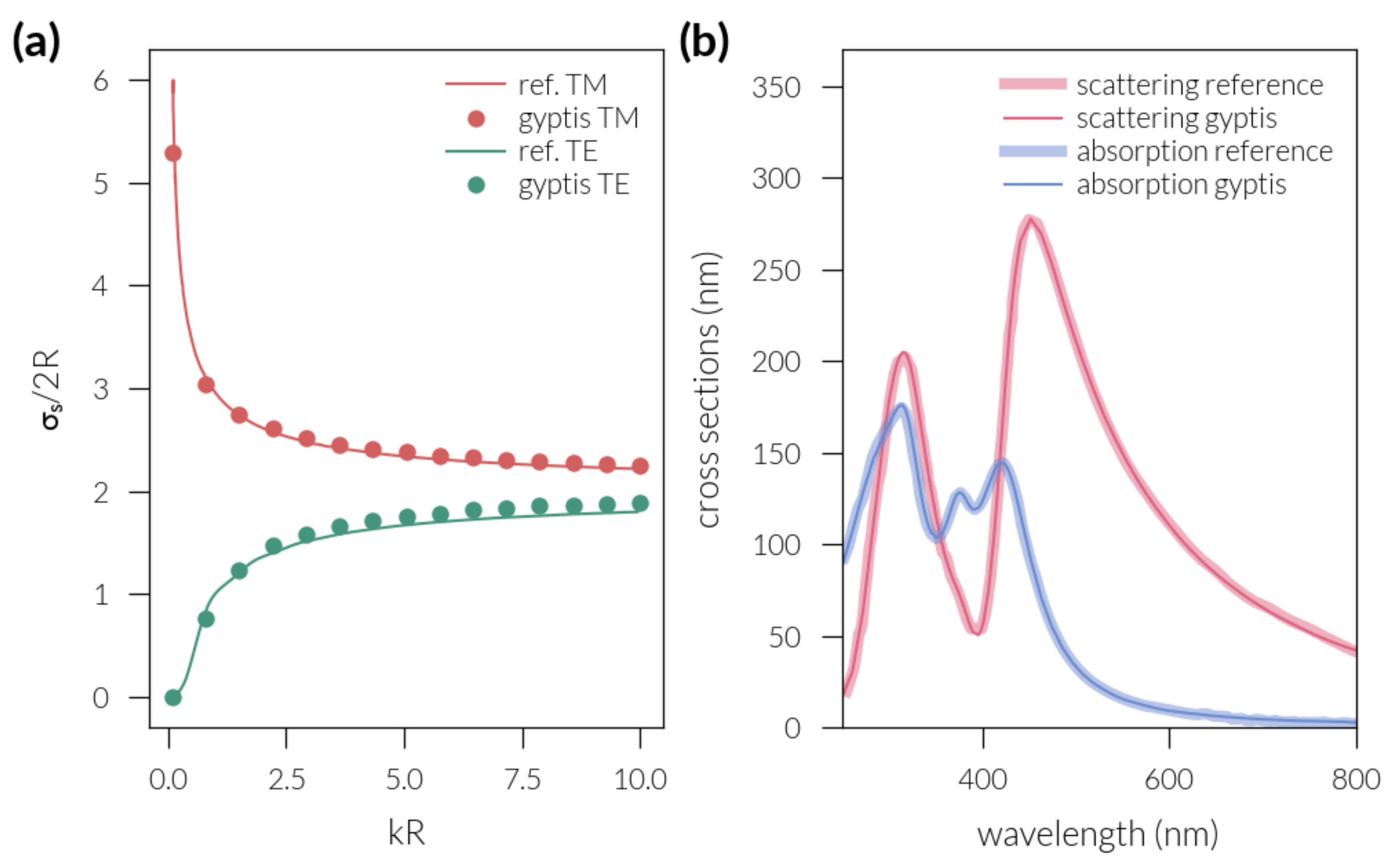
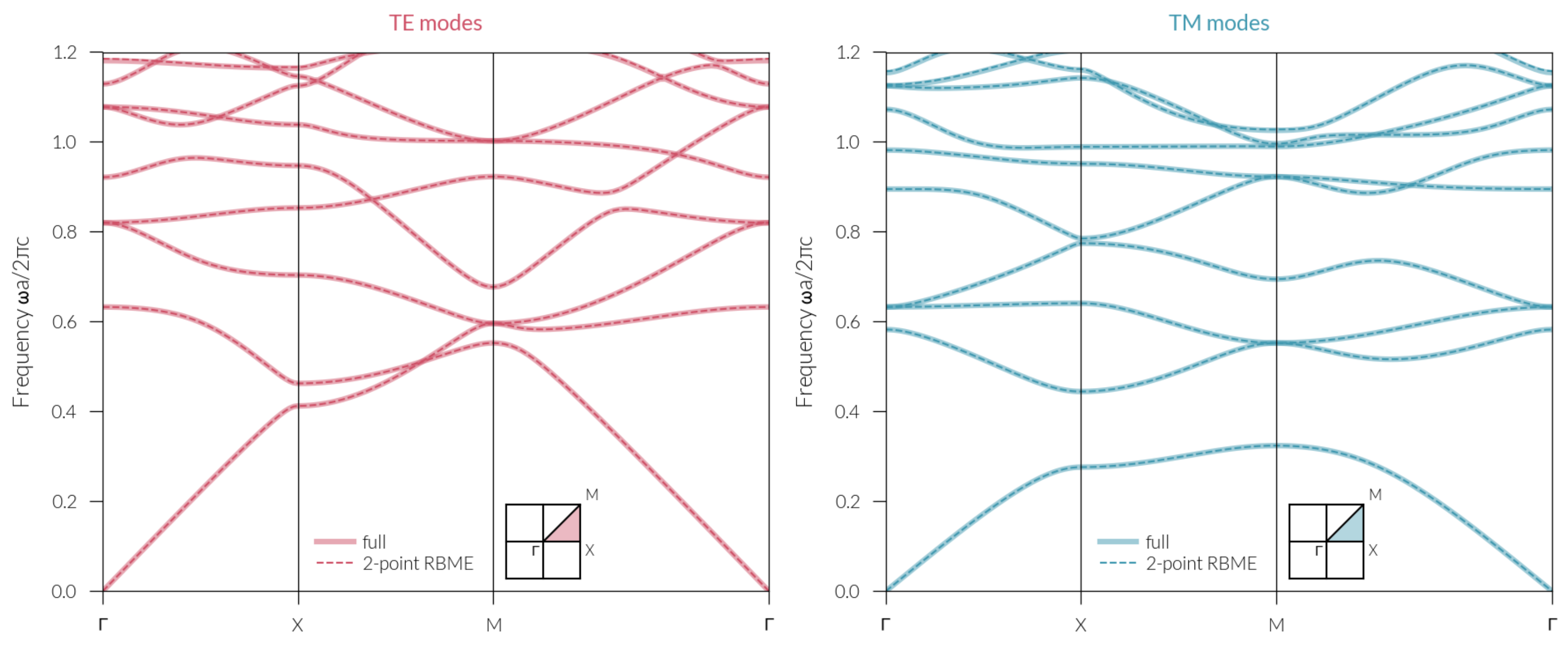
Appendix A. Code Validation

We provide here cross-validation of the code with published results for each numerical method. Other examples and comparisons of our implementations are available online:

Appendix A.1. FEM

First, we study the diffraction of a plane wave by a perfectly conducting circular cylinder. Results are plotted in Figure A1a and agree well with those obtained analytically in [73] for both polarizations.
Next, we compare our code for the scattering of a TE polarized plane wave by a core-shell nanocylinder as studied in Ref. [74]. Results are displayed in Figure A1b and show good agreement with the two methods.
Figure A1. (a): Scattering cross-section (SCS) of a perfectly conducting cylinder for a TE (red) and TM (green) polarized plane wave as a function of k R (k is the wavenumber and R the radius of the cylinder). Solid lines are results from [73] and markers are from our FEM implementation. (b): Scattering cross-section (SCS) and absorption cross-section (ACS) of a single silver-coated dielectric nanocylinder ( ε = 2 ). The inner radius is R 1 = 60 nm, outer radius R 2 = 30 nm. Wider lines are results from [74] and thin solid lines are from our FEM implementation.
Mathematics 10 03912 g0a1

Appendix A.2. FMM

We study here a checkerboard grating made of square unit cells of size d = 2.5 λ 0 , with square inclusion rotated at 45° of permittivity 2.25 (this corresponds to unit cell B in Ref. [25]). The thickness of the structured layer is h = λ 0 , the inclusions are embedded in air ( ε = 1 ), and the permittivity of the substrate and superstrate are ε = 1 and ε = 2.25 , respectively. The structure is illuminated by a plane wave at normal incidence ( θ = ϕ = 0 ) polarized parallel to one side of the square inclusion.
Table A1 shows the propagating transmitted orders for 441 harmonics retained in the modal expansion and a 1000 × 1000 discretization of the unit cell and agrees with Table 1 in Ref. [25].
Table A1. Diffraction efficiencies (%) of the transmitted orders of the checkerboard grating studied in [25].
Diffraction Order−101
−14.34512.8166.130
012.81617.76512.816
16.13012.8164.345
We next study the convergence of the (0, −1) transmitted order: Figure A2 shows that the tangent formulation with proper factorization rules converges must faster than the original RCWA formulation. Those results are in line with findings in Refs. [22,25].
Figure A2. Convergence of the (0, −1) transmitted order as a function of truncation number. Blue triangles: original formulation; green circles: tangent formulation.
Mathematics 10 03912 g0a2

Appendix A.3. PWEM

The structure we study here is a square lattice with lattice constant a of dielectric columns, with radius r = 0.2 a and dielectric constant ε = 8.9 in a vacuum. This is the same photonic crystal considered in Ref. [75] (Chapter 5, Figure 2), and our calculations agree very well with those reference results (see Figure A3). Furthermore, the agreement between the full model and the reduced Bloch mode expansion is good, albeit with a slight discrepancy for higher frequency bands, but the RBME calculation is more than eight times faster.
Figure A3. The photonic band structure for a square array of dielectric columns. The insets show the Brillouin zone, with the irreducible zone shaded. Solid lines are results from the full model and dashed lines are results obtained with the reduced Bloch mode expansion. Here we retained 385 plane waves in the expansion and used the first 8 modes calculated at the three symmetry points Γ , X, and M for the RBME. The path in reciprocal space is discretized with 144 points.
Mathematics 10 03912 g0a3

References

  1. Bendsoe, M.P.; Sigmund, O. Topology Optimization: Theory, Methods, and Applications; Springer: Berlin/Heidelberg, Germany, 2013. [Google Scholar]
  2. Molesky, S.; Lin, Z.; Piggott, A.Y.; Jin, W.; Vucković, J.; Rodriguez, A.W. Inverse Design in Nanophotonics. Nat. Photonics 2018, 12, 659–670. [Google Scholar] [CrossRef] [Green Version]
  3. Andkjær, J.; Sigmund, O. Topology Optimized Low-Contrast All-Dielectric Optical Cloak. Appl. Phys. Lett. 2011, 98, 021112. [Google Scholar] [CrossRef] [Green Version]
  4. Vial, B.; Hao, Y. Topology Optimized All-Dielectric Cloak: Design, Performances and Modal Picture of the Invisibility Effect. Opt. Express 2015, 23, 23551. [Google Scholar] [CrossRef] [PubMed]
  5. Vial, B.; Torrico, M.M.; Hao, Y. Optimized Microwave Illusion Device. Sci. Rep. 2017, 7, 3929. [Google Scholar] [CrossRef] [PubMed]
  6. Jensen, J.S.; Sigmund, O. Systematic Design of Photonic Crystal Structures Using Topology Optimization: Low-Loss Waveguide Bends. Appl. Phys. Lett. 2004, 84, 2022–2024. [Google Scholar] [CrossRef] [Green Version]
  7. Jensen, J.S.; Sigmund, O. Topology Optimization of Photonic Crystal Structures: A High-Bandwidth Low-Loss T-Junction Waveguide. J. Opt. Soc. Am. Opt. Phys. 2005, 22, 1191. [Google Scholar] [CrossRef]
  8. Diaz, A.R.; Sigmund, O. A Topology Optimization Method for Design of Negative Permeability Metamaterials. Struct. Multidisc. Optim. 2009, 41, 163–177. [Google Scholar] [CrossRef]
  9. Nishi, S.; Yamada, T.; Izui, K.; Nishiwaki, S.; Terada, K. Isogeometric Topology Optimization of Anisotropic Metamaterials for Controlling High-Frequency Electromagnetic Wave. Int. J. Numer. Methods Eng. 2020, 121, 1218–1247. [Google Scholar] [CrossRef]
  10. Lin, Z.; Liu, V.; Pestourie, R.; Johnson, S.G. Topology Optimization of Freeform Large-Area Metasurfaces. Opt. Express 2019, 27, 15765–15775. [Google Scholar] [CrossRef] [Green Version]
  11. Fan, J.A. Freeform Metasurface Design Based on Topology Optimization. MRS Bull. 2020, 45, 196–201. [Google Scholar] [CrossRef]
  12. Pestourie, R.; Pérez-Arancibia, C.; Lin, Z.; Shin, W.; Capasso, F.; Johnson, S.G. Inverse Design of Large-Area Metasurfaces. Opt. Express 2018, 26, 33732–33747. [Google Scholar] [CrossRef]
  13. Christiansen, R.E.; Christiansen, R.E.; Sigmund, O.; Sigmund, O. Inverse Design in Photonics by Topology Optimization: Tutorial. JOSA B 2021, 38, 496–509. [Google Scholar] [CrossRef]
  14. Jensen, J.; Sigmund, O. Topology Optimization for Nano-Photonics. Laser Photon. Rev. 2010, 5, 308–321. [Google Scholar] [CrossRef]
  15. Demésy, G.; Zolla, F.; Nicolet, A.; Commandré, M.; Fossati, C. The Finite Element Method as Applied to the Diffraction by an Anisotropic Grating. Opt. Express 2007, 15, 18089–18102. [Google Scholar] [CrossRef]
  16. Berenger, J.P. A Perfectly Matched Layer for the Absorption of Electromagnetic Waves. J. Comput. Phys. 1994, 114, 185–200. [Google Scholar] [CrossRef]
  17. Vial, B.; Zolla, F.; Nicolet, A.; Commandré, M.; Tisserand, S. Adaptive Perfectly Matched Layer for Wood’s Anomalies in Diffraction Gratings. Opt. Express 2012, 20, 28094. [Google Scholar] [CrossRef] [Green Version]
  18. Vial, B. Gyptis. Zenodo. 2022. Available online: https://zenodo.org/record/6636134#.Y1CkJExBxPY (accessed on 17 October 2022).
  19. Geuzaine, C.; Remacle, J.F. Gmsh: A 3-D Finite Element Mesh Generator with Built-in Pre- and Post-Processing Facilities. Int. J. Numer. Methods Eng. 2009, 79, 1309–1331. [Google Scholar] [CrossRef]
  20. Alnæs, M.; Blechta, J.; Hake, J.; Johansson, A.; Kehlet, B.; Logg, A.; Richardson, C.; Ring, J.; Rognes, M.E.; Wells, G.N. Archive of Numerical Software. The FEniCS Project Version 1.5. 2015. Available online: https://journals.ub.uni-heidelberg.de/index.php/ans/article/view/20553 (accessed on 17 October 2022).
  21. Whittaker, D.M.; Culshaw, I.S. Scattering-Matrix Treatment of Patterned Multilayer Photonic Structures. Phys. Rev. B 1999, 60, 2610–2618. [Google Scholar] [CrossRef] [Green Version]
  22. Liu, V.; Fan, S. S4: A Free Electromagnetic Solver for Layered Periodic Structures. Comput. Phys. Commun. 2012, 183, 2233–2244. [Google Scholar] [CrossRef]
  23. Popov, E.; Nevière, M. Maxwell Equations in Fourier Space: Fast-Converging Formulation for Diffraction by Arbitrary Shaped, Periodic, Anisotropic Media. JOSA A 2001, 18, 2886–2894. [Google Scholar] [CrossRef]
  24. Moharam, M.G.; Gaylord, T.K. Rigorous Coupled-Wave Analysis of Planar-Grating Diffraction. JOSA 1981, 71, 811–818. [Google Scholar] [CrossRef]
  25. Li, L. New Formulation of the Fourier Modal Method for Crossed Surface-Relief Gratings. JOSA A 1997, 14, 2758–2767. [Google Scholar] [CrossRef]
  26. Schuster, T.; Ruoff, J.; Kerwien, N.; Rafler, S.; Osten, W. Normal Vector Method for Convergence Improvement Using the RCWA for Crossed Gratings. JOSA A 2007, 24, 2880–2890. [Google Scholar] [CrossRef] [PubMed]
  27. Götz, P.; Schuster, T.; Frenner, K.; Rafler, S.; Osten, W. Normal Vector Method for the RCWA with Automated Vector Field Generation. Opt. Express 2008, 16, 17295–17301. [Google Scholar] [CrossRef]
  28. Li, L. Fourier Modal Method for Crossed Anisotropic Gratings with Arbitrary Permittivity and Permeability Tensors. J. Opt. Pure Appl. Opt. 2003, 5, 345–355. [Google Scholar] [CrossRef]
  29. Li, L. Formulation and Comparison of Two Recursive Matrix Algorithms for Modeling Layered Diffraction Gratings. JOSA A 1996, 13, 1024–1035. [Google Scholar] [CrossRef] [Green Version]
  30. Hussein, M.I. Reduced Bloch Mode Expansion for Periodic Media Band Structure Calculations. Proc. R. Soc. Math. Phys. Eng. Sci. 2009, 465, 2825–2848. [Google Scholar] [CrossRef] [Green Version]
  31. Griewank, A.; Walther, A. Evaluating Derivatives; Other Titles in Applied Mathematics; Society for Industrial and Applied Mathematics: Philadelphia, PA, USA, 2008. [Google Scholar] [CrossRef]
  32. Corliss, G.; Faure, C.; Griewank, A.; Hascoet, L.; Naumann, U. Automatic Differentiation of Algorithms: From Simulation to Optimization; Springer: Berlin/Heidelberg, Germany, 2013. [Google Scholar]
  33. Baydin, A.G.; Pearlmutter, B.A.; Radul, A.A.; Siskind, J.M. Automatic Differentiation in Machine Learning: A Survey. J. Mach. Learn. Res. 2017, 18, 5595–5637. [Google Scholar]
  34. Mitusch, S.K.; Funke, S.W.; Dokken, J.S. Dolfin-Adjoint 2018.1: Automated Adjoints for FEniCS and Firedrake. J. Open Source Softw. 2019, 4, 1292. [Google Scholar] [CrossRef]
  35. Harris, C.R.; Millman, K.J.; van der Walt, S.J.; Gommers, R.; Virtanen, P.; Cournapeau, D.; Wieser, E.; Taylor, J.; Berg, S.; Smith, N.J.; et al. Array Programming with NumPy. Nature 2020, 585, 357–362. [Google Scholar] [CrossRef]
  36. Virtanen, P.; Gommers, R.; Oliphant, T.E.; Haberland, M.; Reddy, T.; Cournapeau, D.; Burovski, E.; Peterson, P.; Weckesser, W.; Bright, J.; et al. SciPy 1.0: Fundamental Algorithms for Scientific Computing in Python. Nat. Methods 2020, 17, 261–272. [Google Scholar] [CrossRef] [Green Version]
  37. Bradbury, J.; Frostig, R.; Hawkins, P.; Johnson, M.J.; Leary, C.; Maclaurin, D.; Necula, G.; Paszke, A.; VanderPlas, J.; Wanderman-Milne, S.; et al. JAX: Composable Transformations of Python+NumPy Programs. 2018. Available online: https://github.com/google/jax3 (accessed on 17 October 2022).
  38. Maclaurin, D.; Duvenaud, D.; Adams, R.P. Autograd: Effortless Gradients in Numpy. Proc. ICML 2015, 238, 5. [Google Scholar]
  39. Paszke, A.; Gross, S.; Massa, F.; Lerer, A.; Bradbury, J.; Chanan, G.; Killeen, T.; Lin, Z.; Gimelshein, N.; Antiga, L.; et al. PyTorch: An Imperative Style, High-Performance Deep Learning Library. In Advances in Neural Information Processing Systems 32; Wallach, H., Larochelle, H., Beygelzimer, A., d’Alché-Buc, F., Fox, E., Garnett, R., Eds.; Curran Associates, Inc.: Red Hook, NY, USA, 2019; pp. 8024–8035. [Google Scholar]
  40. Paszke, A.; Gross, S.; Chintala, S.; Chanan, G.; Yang, E.; DeVito, Z.; Lin, Z.; Desmaison, A.; Antiga, L.; Lerer, A. Automatic Differentiation in PyTorch. In Proceedings of the NIPS-W, Long Beach, CA, USA, 9 December 2017. [Google Scholar]
  41. Lazarov, B.S.; Sigmund, O. Filters in Topology Optimization Based on Helmholtz-type Differential Equations. Int. J. Numer. Methods Eng. 2011, 86, 765–781. [Google Scholar] [CrossRef]
  42. Wang, F.; Lazarov, B.S.; Sigmund, O. On Projection Methods, Convergence and Robust Formulations in Topology Optimization. Struct. Multidisc. Optim. 2010, 43, 767–784. [Google Scholar] [CrossRef]
  43. Bendsøe, M.; Sigmund, O. Material Interpolation Schemes in Topology Optimization. Arch. Appl. Mech. Ing. Arch. 1999, 69, 635–654. [Google Scholar] [CrossRef]
  44. Svanberg, K. A Class of Globally Convergent Optimization Methods Based on Conservative Convex Separable Approximations. SIAM J. Optim. 2002, 12, 555–573. [Google Scholar] [CrossRef] [Green Version]
  45. Johnson, S.G. The NLopt Nonlinear-Optimization Package. Available online: http://github.com/stevengj/nlopt (accessed on 17 October 2022).
  46. Aslan, K.; Lakowicz, J.R.; Geddes, C.D. Plasmon Light Scattering in Biology and Medicine: New Sensing Approaches, Visions and Perspectives. Curr. Opin. Chem. Biol. 2005, 9, 538–544. [Google Scholar] [CrossRef]
  47. Guo, X.; Ying, Y.; Tong, L. Photonic Nanowires: From Subwavelength Waveguides to Optical Sensors. Acc. Chem. Res. 2014, 47, 656–666. [Google Scholar] [CrossRef]
  48. Lee, B.; Lee, I.M.; Kim, S.; Oh, D.H.; Hesselink, L. Review on Subwavelength Confinement of Light with Plasmonics. J. Mod. Opt. 2010, 57, 1479–1497. [Google Scholar] [CrossRef]
  49. Powell, A.W.; Mrnka, M.; Hibbins, A.P.; Sambles, J.R. Superscattering and Directive Antennas via Mode Superposition in Subwavelength Core-Shell Meta-Atoms. Photonics 2022, 9, 6. [Google Scholar] [CrossRef]
  50. Wee, W.H.; Pendry, J.B. Shrinking Optical Devices. New J. Phys. 2009, 11, 073033. [Google Scholar] [CrossRef]
  51. Yang, T.; Chen, H.; Luo, X.; Ma, H. Superscatterer: Enhancement of Scattering with Complementary Media. Opt. Express 2008, 16, 18545–18550. [Google Scholar] [CrossRef] [Green Version]
  52. Ruan, Z.; Fan, S. Superscattering of Light from Subwavelength Nanostructures. Phys. Rev. Lett. 2010, 105, 013901. [Google Scholar] [CrossRef]
  53. Ruan, Z.; Fan, S. Design of Subwavelength Superscattering Nanospheres. Appl. Phys. Lett. 2011, 98, 043101. [Google Scholar] [CrossRef] [Green Version]
  54. Mirzaei, A.; Miroshnichenko, A.E.; Shadrivov, I.V.; Kivshar, Y.S. Superscattering of Light Optimized by a Genetic Algorithm. Appl. Phys. Lett. 2014, 105, 011109. [Google Scholar] [CrossRef] [Green Version]
  55. Frezza, F.; Mangini, F.; Tedeschi, N. Introduction to Electromagnetic Scattering: Tutorial. JOSA A 2018, 35, 163–173. [Google Scholar] [CrossRef]
  56. Ching, E.S.C.; Leung, P.T.; Maassen van den Brink, A.; Suen, W.M.; Tong, S.S.; Young, K. Quasinormal-Mode Expansion for Waves in Open Systems. Rev. Mod. Phys. 1998, 70, 1545–1554. [Google Scholar] [CrossRef] [Green Version]
  57. Zolla, F.; Nicolet, A.; Demésy, G. Photonics in Highly Dispersive Media: The Exact Modal Expansion. Opt. Lett. 2018, 43, 5813–5816. [Google Scholar] [CrossRef] [PubMed] [Green Version]
  58. Lalanne, P.; Yan, W.; Gras, A.; Sauvan, C.; Hugonin, J.P.; Besbes, M.; Demésy, G.; Truong, M.D.; Gralak, B.; Zolla, F.; et al. Quasinormal Mode Solvers for Resonators with Dispersive Materials. JOSA A 2019, 36, 686–704. [Google Scholar] [CrossRef] [PubMed]
  59. Vial, B.; Zolla, F.; Nicolet, A.; Commandré, M. Quasimodal Expansion of Electromagnetic Fields in Open Two-Dimensional Structures. Phys. Rev. At. Mol. Opt. Phys. 2014, 89, 023829. [Google Scholar] [CrossRef] [Green Version]
  60. Yu, N.; Genevet, P.; Kats, M.A.; Aieta, F.; Tetienne, J.P.; Capasso, F.; Gaburro, Z. Light Propagation with Phase Discontinuities: Generalized Laws of Reflection and Refraction. Science 2011, 334, 333–337. [Google Scholar] [CrossRef]
  61. Kildishev, A.V.; Boltasseva, A.; Shalaev, V.M. Planar Photonics with Metasurfaces. Science 2013, 339, 1232009. [Google Scholar] [CrossRef] [Green Version]
  62. Sell, D.; Yang, J.; Doshay, S.; Yang, R.; Fan, J.A. Large-Angle, Multifunctional Metagratings Based on Freeform Multimode Geometries. Nano Lett. 2017, 17, 3752–3757. [Google Scholar] [CrossRef]
  63. Lin, Z.; Groever, B.; Capasso, F.; Rodriguez, A.W.; Lončar, M. Topology-Optimized Multilayered Metaoptics. Phys. Rev. Appl. 2018, 9, 044030. [Google Scholar] [CrossRef] [Green Version]
  64. Roques-Carmes, C.; Lin, Z.; Christiansen, R.E.; Salamin, Y.; Kooi, S.E.; Joannopoulos, J.D.; Johnson, S.G.; Soljačić, M. Toward 3D-Printed Inverse-Designed Metaoptics. ACS Photonics 2022, 9, 43–51. [Google Scholar] [CrossRef]
  65. Yang, J.; Fan, J.A. Topology-Optimized Metasurfaces: Impact of Initial Geometric Layout. Opt. Lett. 2017, 42, 3161–3164. [Google Scholar] [CrossRef]
  66. Sigmund, O.; Hougaard, K. Geometric Properties of Optimal Photonic Crystals. Phys. Rev. Lett. 2008, 100, 153904. [Google Scholar] [CrossRef] [Green Version]
  67. Men, H.; Lee, K.Y.K.; Freund, R.M.; Peraire, J.; Johnson, S.G. Robust Topology Optimization of Three-Dimensional Photonic-Crystal Band-Gap Structures. Opt. Express 2014, 22, 22632–22648. [Google Scholar] [CrossRef] [Green Version]
  68. Minkov, M.; Williamson, I.A.D.; Andreani, L.C.; Gerace, D.; Lou, B.; Song, A.Y.; Hughes, T.W.; Fan, S. Inverse Design of Photonic Crystals through Automatic Differentiation. ACS Photonics 2020, 7, 1729–1741. [Google Scholar] [CrossRef]
  69. Vercruysse, D.; Sapra, N.V.; Su, L.; Vuckovic, J. Dispersion Engineering with Photonic Inverse Design. IEEE J. Sel. Top. Quantum Electron. 2020, 26, 1–6. [Google Scholar] [CrossRef]
  70. Lin, Z.; Pick, A.; Lončar, M.; Rodriguez, A.W. Enhanced Spontaneous Emission at Third-Order Dirac Exceptional Points in Inverse-Designed Photonic Crystals. Phys. Rev. Lett. 2016, 117, 107402. [Google Scholar] [CrossRef]
  71. Vial, B. Nannos. Zenodo. 2022. Available online: https://doi.org/10.5281/zenodo.6636104 (accessed on 17 October 2022).
  72. Vial, B. Protis. Zenodo. 2022. Available online: https://doi.org/10.5281/zenodo.6636141 (accessed on 17 October 2022).
  73. Ruppin, R. Scattering of Electromagnetic Radiation by a Perfect Electromagnetic Conductor Cylinder. J. Electromagn. Waves Appl. 2006, 20, 1853–1860. [Google Scholar] [CrossRef]
  74. Jandieri, V.; Meng, P.; Yasumoto, K.; Liu, Y. Scattering of Light by Gratings of Metal-Coated Nanocylinders on Dielectric Substrate. J. Opt. Soc. Am. A 2015, 32, 1384. [Google Scholar] [CrossRef]
  75. Joannopoulos, J.D.; Johnson, S.G.; Winn, J.N.; Meade, R.D. Photonic Crystals: Molding the Flow of Light, 2nd ed.; Princeton University Press: Princeton, NJ, USA, 2008. [Google Scholar]
Figure 1. Optimized superscattering nanorods. (a): normalized scattering width as a function of the wavelength of the incident light (blue: TE polarization, red: TM polarization). The insets at the top show the optimized dielectric distribution (white for SiO2 and black for Si), and the bottom insets are the radiation patterns for the normalized scattering width, in dB. The field maps on the right panels show the square norm of the fields at the target wavelength λ 0 = 600 nm. (b): the square norm of the magnetic field | H z | 2 for TE polarization. (c): square norm of the electric field | E z | 2 for TM polarization.
Mathematics 10 03912 g001
Figure 2. Modal analysis of optimized supperscatterers for TE (left panel) and TM (right panel) polarization. The curves are the coupling coefficients as a function of incident wavelength for the four dominant eigenmodes (those with the highest | C n | at λ = 600 nm ). The insets show the real part of the eigenfield v n for the corresponding QNMs, its resonant wavelength λ n = 2 π / Re   ( k n ) , and quality factor Q n = Re   ( k n ) / 2   Im   ( k n ) .
Mathematics 10 03912 g002
Figure 3. Optimized metasurface blazed in the ( 1 , 0 ) transmitted order. (a): optimization history showing the figure of merit Φ (black squares) and the transmission coefficient for TE (blue line) and TM (red line) polarization. The final metagrating has 90.9% and 85.5% transmission efficiency for TE and TM polarized waves, respectively. (b): optimized density function (0 corresponds to air and 1 to silicon).
Mathematics 10 03912 g003
Figure 4. Transmission spectra in the ( 1 , 0 ) order for the optimized metasurface as a function of wavelength for TE (blue curve) and TM polarization (red curve). The insets show the norm of the Poynting vector (colourmap) and its transverse components (arrows) at the target wavelength directly above the metasurface ( z = 350 nm).
Mathematics 10 03912 g004
Figure 5. Inverse designed two-dimensional photonic crystals. (a): maximal band gap between bands 5 and 6 for TE polarization. The band diagram is computed on the edges of the first Brillouin zone, and the optimized metamaterial exhibits a relative bandgap width of around 26% centred at ω 0 = 0.766 × 2 π c / a . (b): dispersion engineering to obtain a prescribed target (grey dashed lines) for the 6th TM mode (black line). The insets show the optimized unit cell with air (light shades) and dielectric (dark shades).
Mathematics 10 03912 g005
Publisher’s Note: MDPI stays neutral with regard to jurisdictional claims in published maps and institutional affiliations.

