

Numerical Investigation into the Effects of a Viscous Fluid Seabed on Wave Scattering with a Fixed Rectangular Obstacle


Abstract
1. Introduction
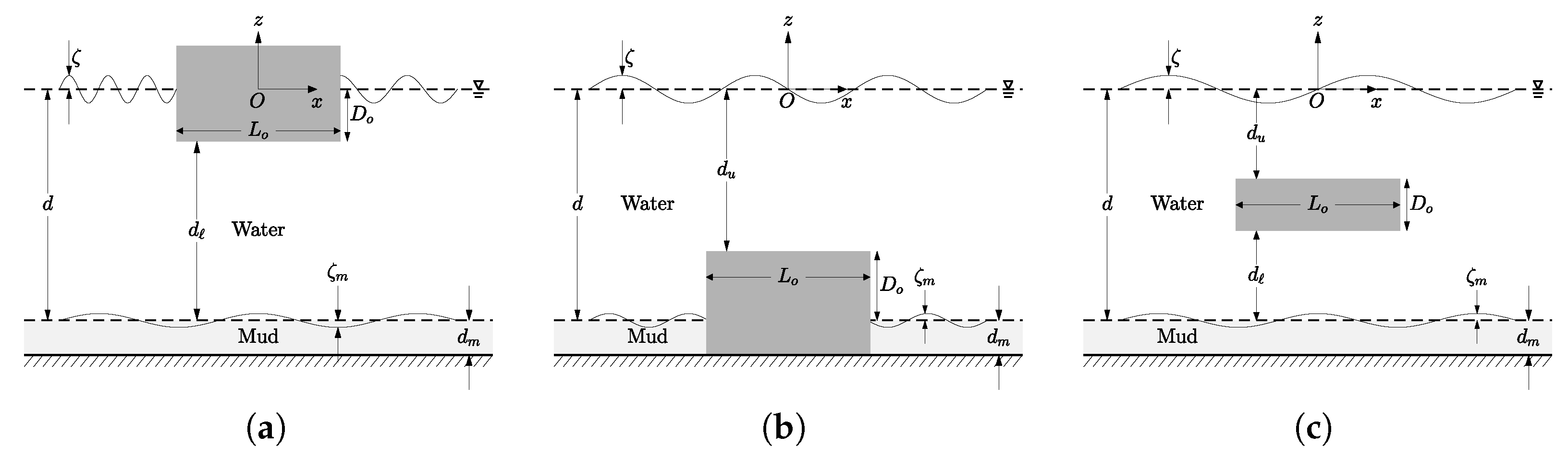
2. Model Development
2.1. Assumptions and Simplifications
2.2. Numerical Model
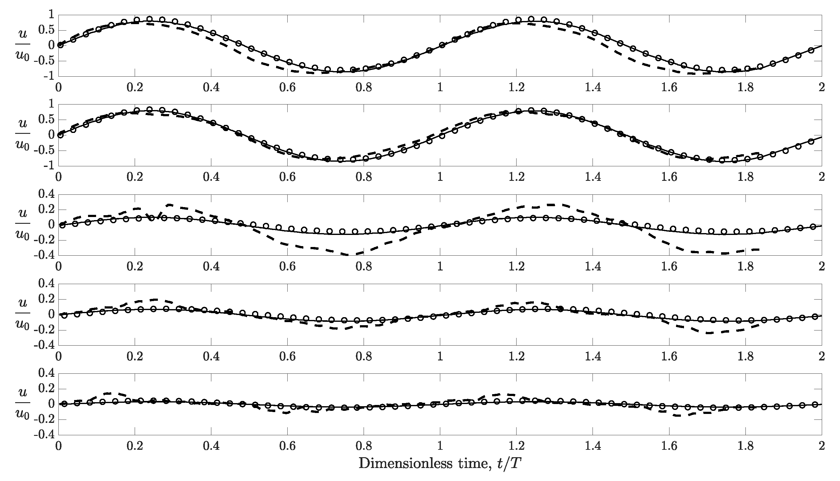
2.3. Model Validation
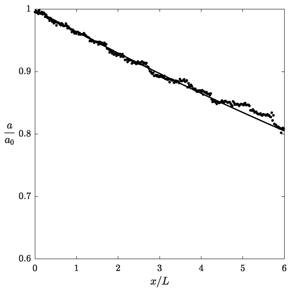
2.3.1. Surface Obstacle above a Solid Bed
2.3.2. Bottom Obstacle on a Solid Bed
2.3.3. Submerged Obstacle above a Solid Bottom
2.3.4. Waves over a Layer of Viscous Fluid Mud
3. Results and Discussions
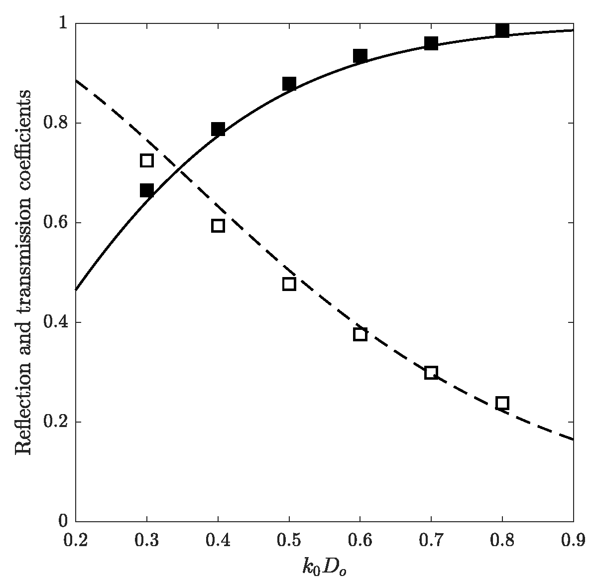
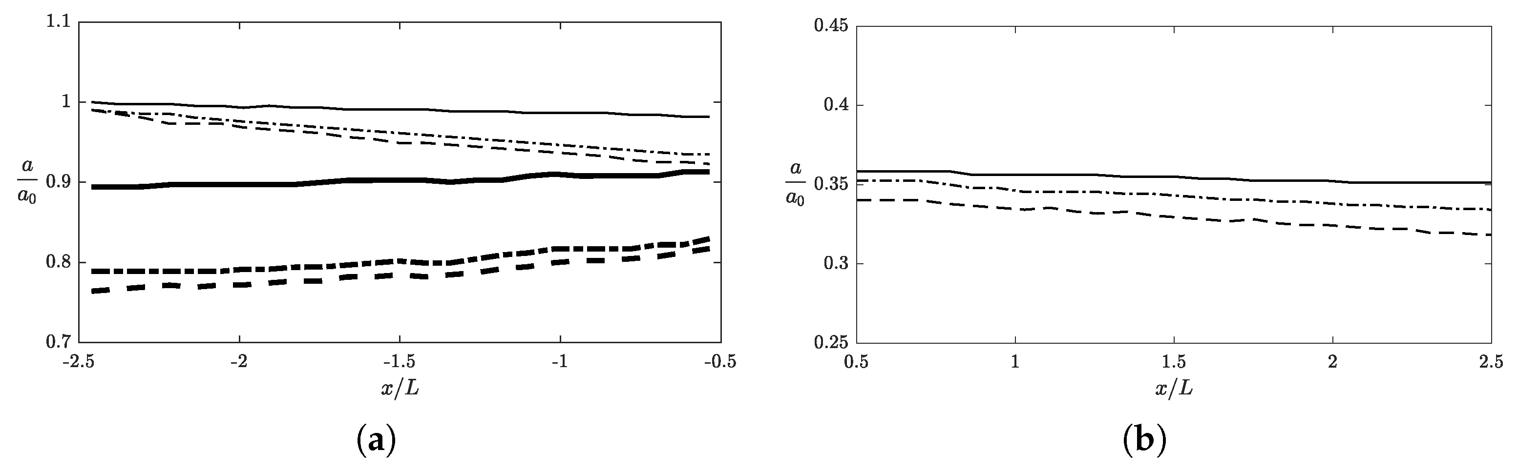
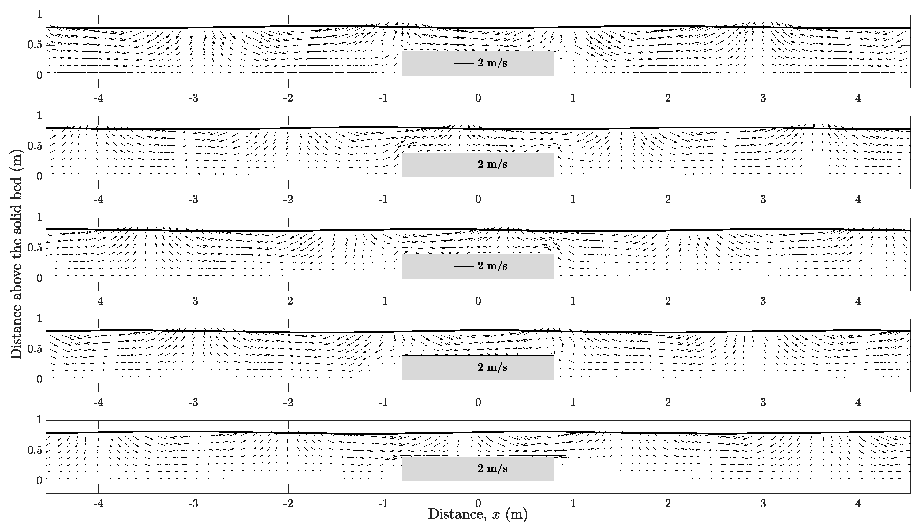
3.1. Surface Obstacle
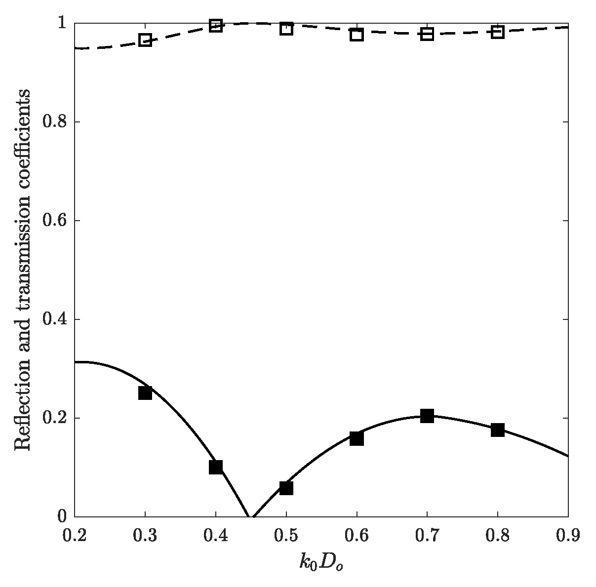
3.2. Bottom Obstacle
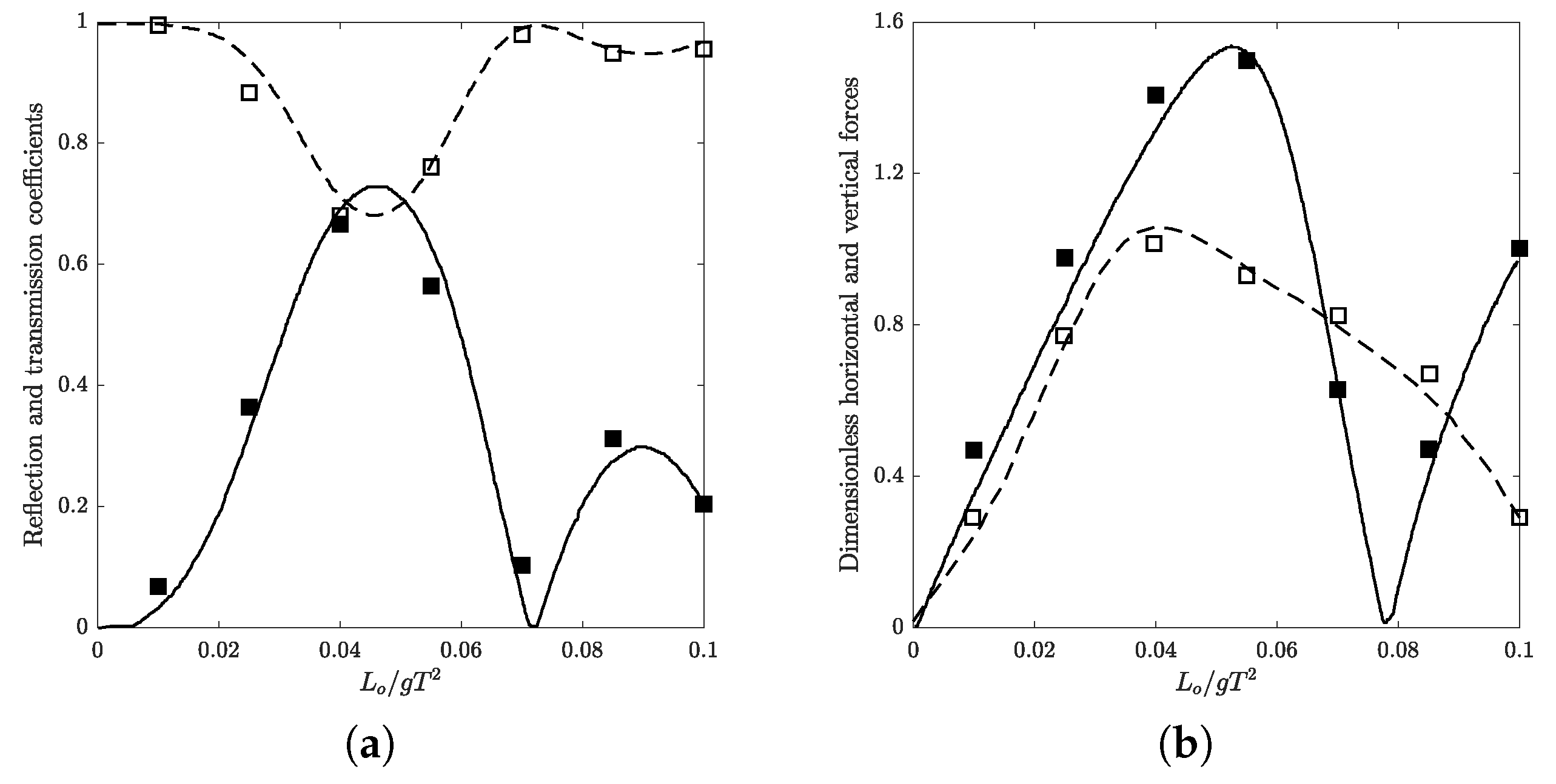
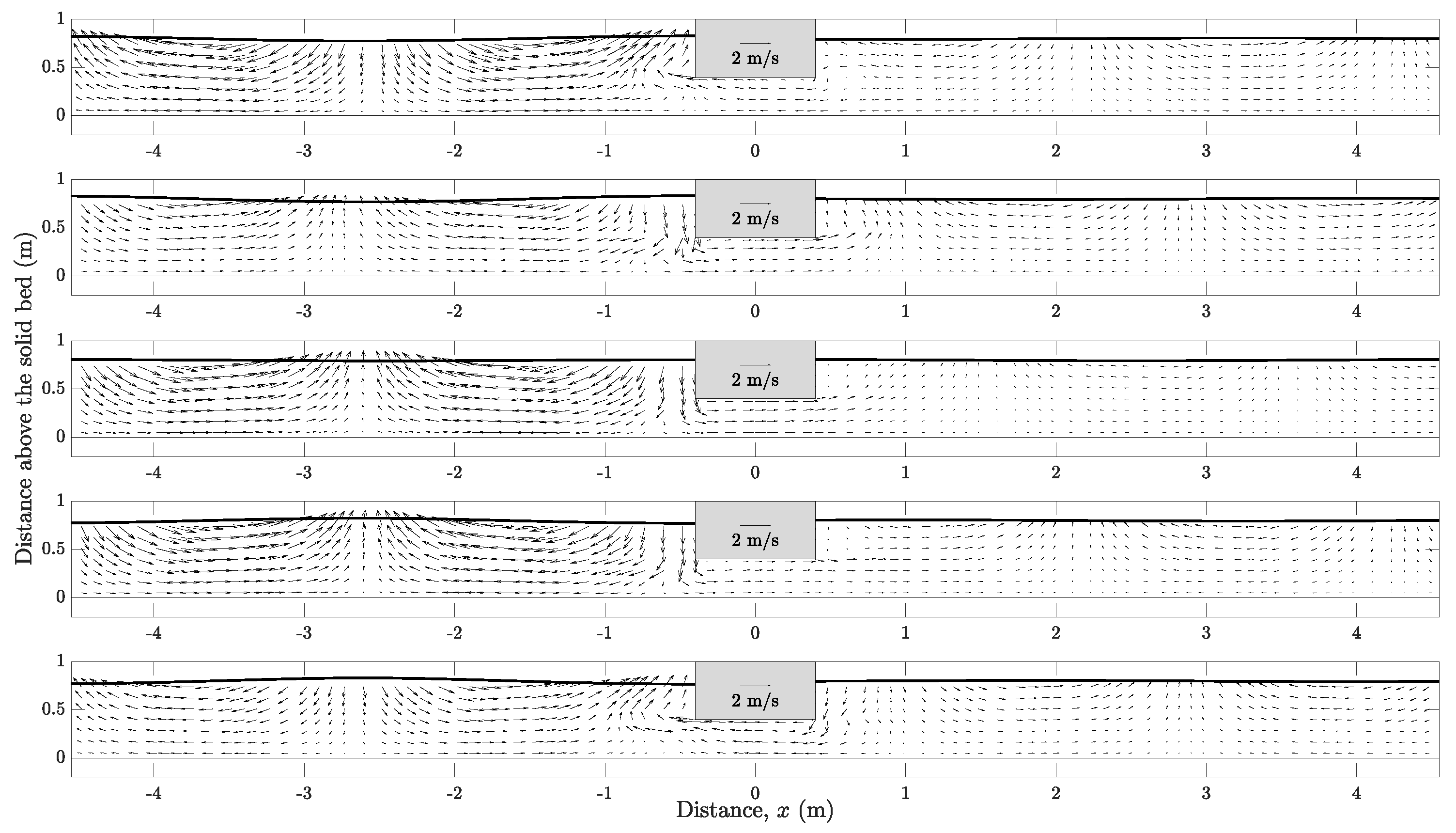
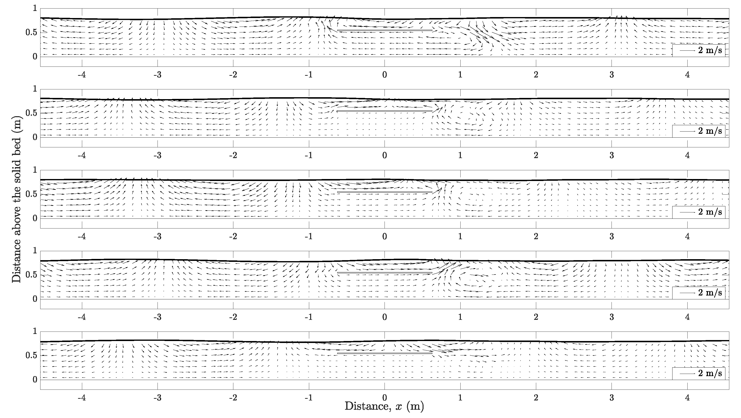
3.3. Submerged Obstacle
4. Concluding Remarks
- Surface obstacle: Section 3.1
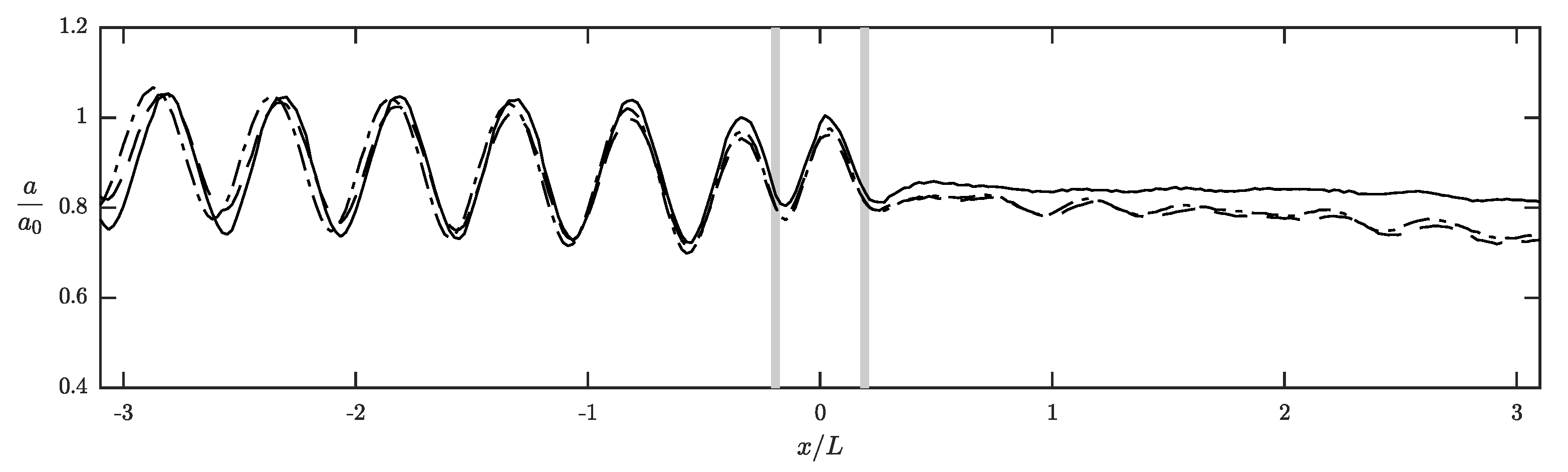
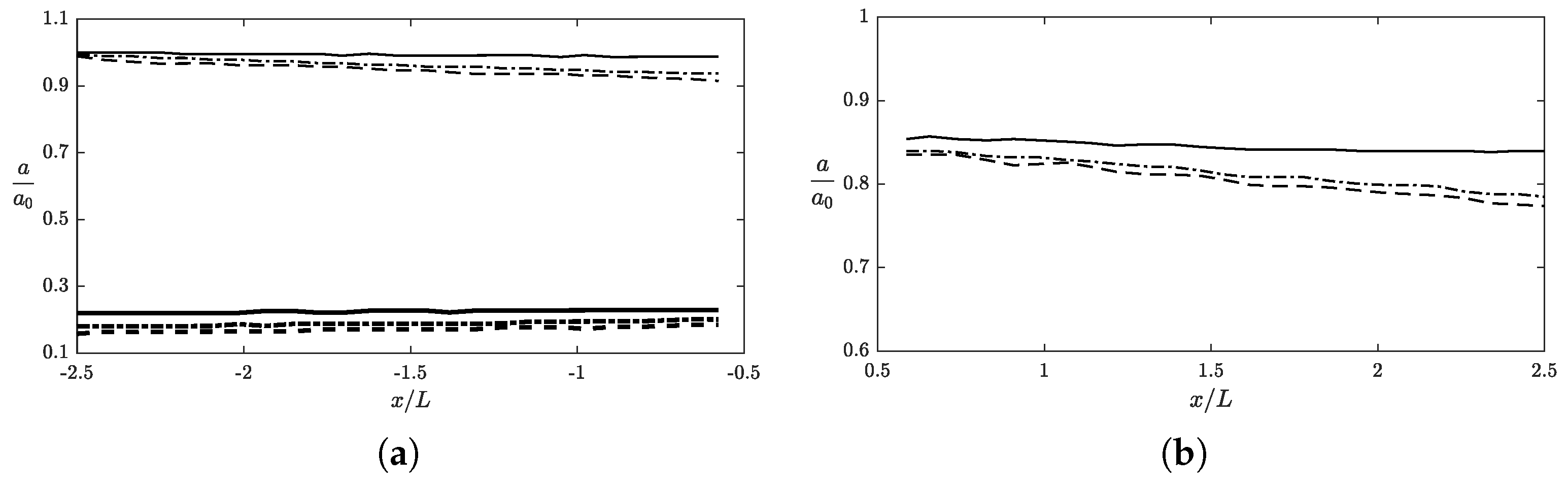
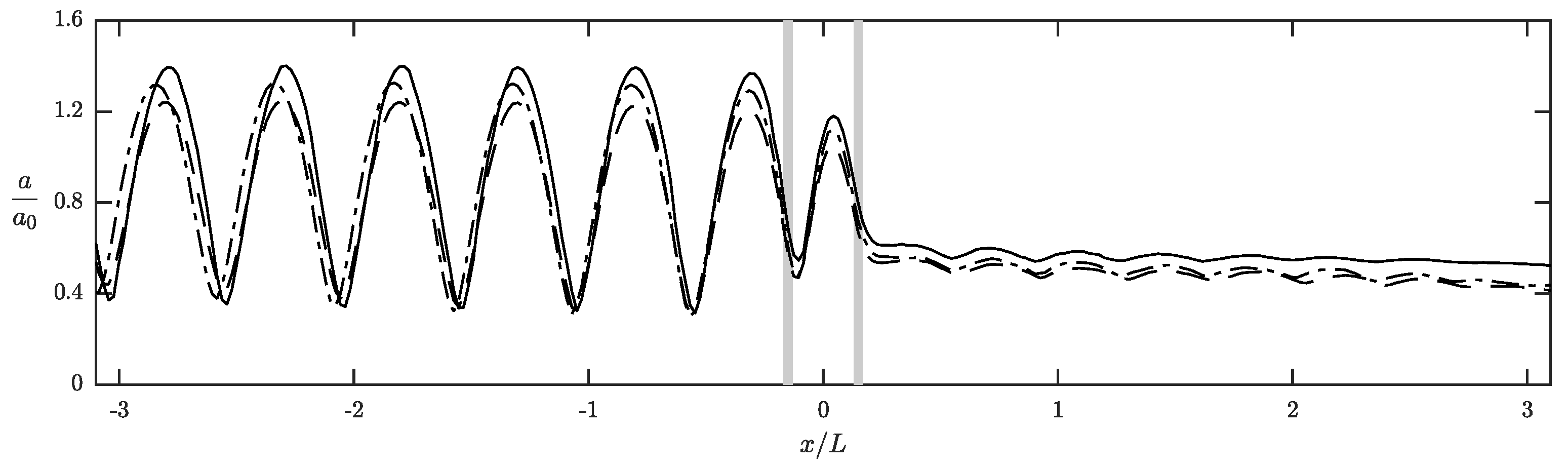
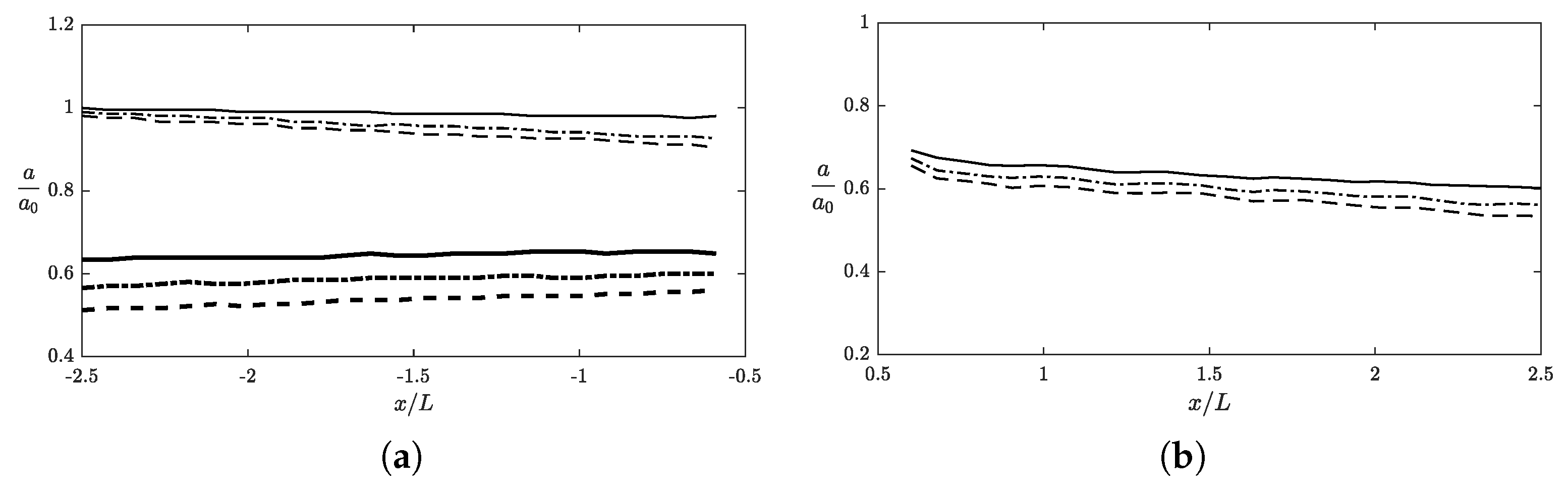
- Incident and transmitted wave components show an amplitude attenuation rate similar to the case of waves over a muddy bed without any obstacles. Reflected waves have a much stronger damping rate.
- For incident, reflected, and transmitted wave components, the largest damping rates all occur at .
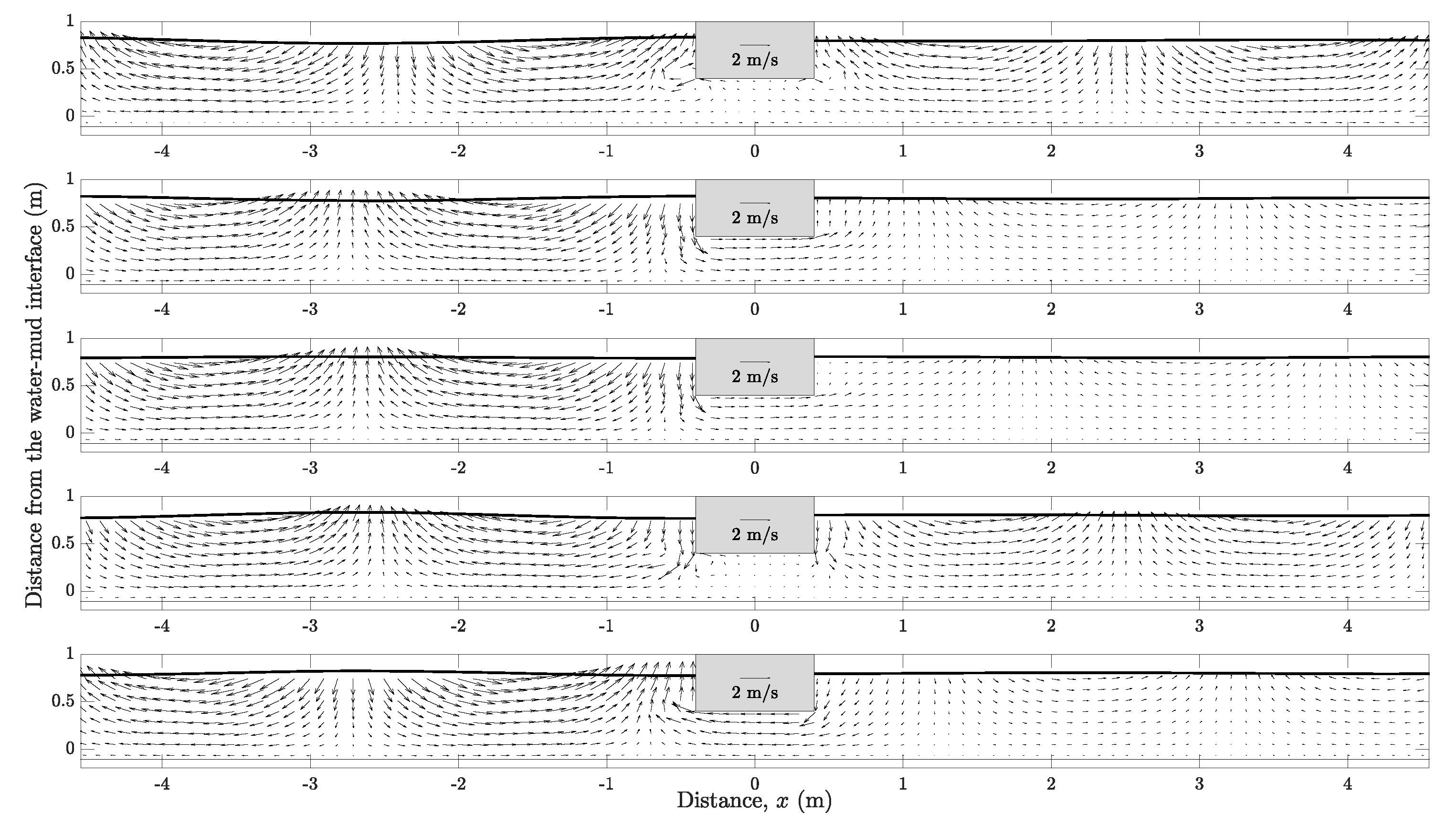
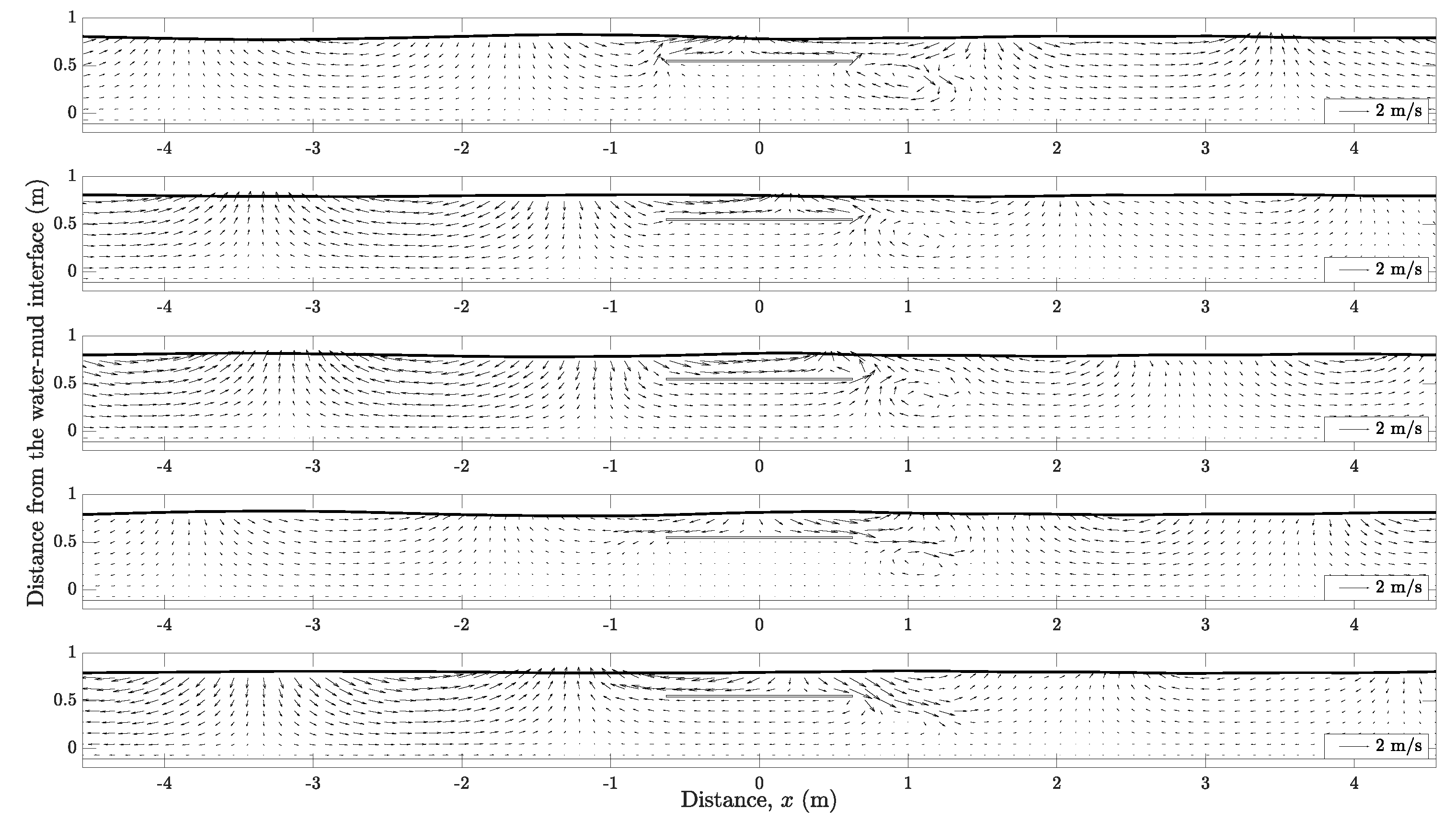
- The pattern of the velocity distribution is mainly controlled by the obstacle with modulation in magnitude and wavelength contributed by the muddy bed.
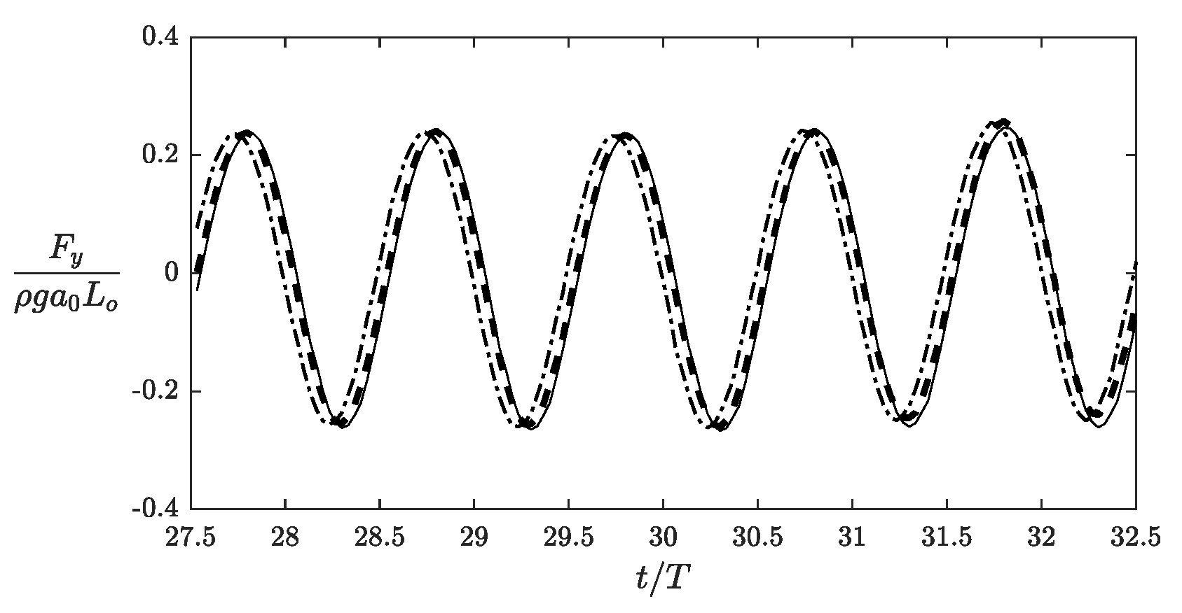
- In terms of the dimensionless vertical wave force exerted on the obstacle surface, a larger phase difference was observed for the case of a thicker mud layer.
- Bottom obstacle: Section 3.2
- The effect of bottom obstacle on mud-induced amplitude attenuation is only considerable for the reflected wave components.
- The largest wave damping of each wave component was observed when the mud layer thickness was .
- The impact of viscous fluid bed on the flow pattern in the vicinity of the obstacle was not obvious. However, a phase shift and increase in wavelength are both more evident.
- A thicker mud layer causes a larger phase lag in the dimensionless vertical wave force on the obstacle surface.
- Submerged obstacle: Section 3.3
- Due to the vortex generated in the lee of the obstacle of the obstacle, a significantly larger decrease in wave amplitude is shown for transmitted wave component. This is very different from the behaviors observed in the cases of surface or bottom obstacles.
- The largest amplitude attenuation rate occurs at for every wave component.
- With the consideration of a viscous fluid mud bed, the size of the vortex core is considerably smaller and the phase difference on the formation of the vortex can also be observed.
- The case with shows a larger decrease in the dimensionless vertical wave force on the obstacle surface. However, the phase shift is more substantial for a thicker layer with .
Author Contributions
Funding
Conflicts of Interest
References
- Sorensen, R.M. Basic Coastal Engineering; Springer: New York, NY, USA, 2006; pp. 209–214. [Google Scholar]
- Bea, R.G.; Iversen, R.; Xu, T. Wave-in-deck forces on offshore platforms. J. Offshore Mech. Arct. Eng. 2001, 123, 10–21. [Google Scholar] [CrossRef]
- Chella, M.A.; Tørum, A.; Myrhaug, D. An overview of wave impact forces on offshore wind turbine substructures. Energy Procedia 2012, 20, 217–226. [Google Scholar] [CrossRef]
- Kunisu, H. Evaluation of wave force acting on submerged floating tunnels. Procedia Eng. 2010, 4, 99–105. [Google Scholar] [CrossRef]
- Liu, Y.; Zheng, S.; Liang, H.; Cong, P. Wave interaction and energy absorption from arrays of complex-shaped point absorbers. Phys. Fluids. 2022, 34, 097107. [Google Scholar] [CrossRef]
- Guo, X.; Wang, B.; Mei, C.C.; Liu, H. Scattering of periodic surface waves by pile-group supported platform. Ocean Eng. 2017, 146, 46–58. [Google Scholar] [CrossRef]
- Mei, C.C.; Black, J.L. Scattering of surface waves by rectangular obstacles in waters of finite depth. J. Fluid Mech. 1969, 38, 499–511. [Google Scholar] [CrossRef]
- Siew, P.F.; Hurley, D.G. Long surface waves incident on a submerged horizontal plate. J. Fluid Mech. 1977, 83, 141–151. [Google Scholar] [CrossRef]
- Ijima, T.; Ozaki, S.; Eguchi, Y.; Kobayashi, A. Breakwater and quay well by horizontal plates. In Proceedings of the 12th Conference on Coastal Engineering, Washington, DC, USA, 13–18 September 1970; pp. 1537–1556. [Google Scholar]
- Liu, P.L.-F.; Iskandarani, M. Scattering of short-wave groups by submerged horizontal plate. J. Waterw. Port Coast. Ocean Eng. 1991, 117, 235–246. [Google Scholar] [CrossRef]
- Cheong, H.-F.; Shankar, N.J.; Nallayarasu, S. Analysis of submerged platform breakwater by eigenfunction expansion method. Oecan Eng. 1996, 23, 649–666. [Google Scholar] [CrossRef]
- Bautista, E.; Bahena-Jimenez, S.; Quesada-Torres, A.; Méndez, F.; Arcos, E. Interaction between long water waves and two fixed submerged breakwaters of wavy surfaces. Wave Motion 2022, 112, 102926. [Google Scholar] [CrossRef]
- Williams, K.J. An experimental study of wave-obstacle interaction in a two-dimensional domain. J. Hydraul. Res. 1988, 26, 463–482. [Google Scholar] [CrossRef]
- Murali, K.; Mani, J.S. Performance of Cage Floating Breakwater. J. Waterw. Port Coast. Ocean Eng. 1997, 123, 172–179. [Google Scholar] [CrossRef]
- Kagemoto, H.; Fujino, M.; Murai, M. Theoretical and experimental predictions of the hydroelastic response of a very large floating structure in waves. Appl. Ocean Res. 1998, 26, 135–144. [Google Scholar] [CrossRef]
- Martinelli, L.; Ruol, P.; Zanuttigh, B. Wave basin experiments on floating breakwaters with different layouts. Appl. Ocean Res. 2008, 30, 199–207. [Google Scholar] [CrossRef]
- Jalos, P. The passage of waves over a bar. Houille Blanche 1960, 15, 247–267. [Google Scholar]
- Dick, T.M.; Brebner, A. Solid and permeable submerged breakwaters. In Proceedings of the 11th Conference on Coastal Engineering, London, UK, 16–20 September 1968; pp. 1141–1158. [Google Scholar]
- Rey, V.; Belzons, M.; Guazzelli, E. Propagation of surface gravity waves over a rectangular submerged bar. J. Fluid Mech. 1992, 235, 453–479. [Google Scholar] [CrossRef]
- Ting, F.C.K.; Kim, Y.-K. Vortex generation in water waves propagating over a submerged obstacle. Coast. Eng. 1994, 24, 23–49. [Google Scholar] [CrossRef]
- Chang, K.-A.; Hsu, T.-J.; Liu, P.L.-F. Vortex generation and evolution in water waves propagating over a submerged rectangular obstacle: Part I. Solitary waves. Coast. Eng. 2001, 44, 13–36. [Google Scholar] [CrossRef]
- Chang, K.-A.; Hsu, T.-J.; Liu, P.L.-F. Vortex generation and evolution in water waves propagating over a submerged rectangular obstacle: Part II: Cnoidal waves. Coast. Eng. 2005, 52, 257–283. [Google Scholar] [CrossRef]
- Rey, V.; Touboul, J. Forces and moment on a horizontal plate due to regular and irregular waves in the presence of current. Appl. Ocean Res. 2011, 33, 88–99. [Google Scholar] [CrossRef]
- Durgin, W.W.; Shiau, J.C. Wave induced pressures on submerged plates. J. Waterways Harbors Coast. Eng. 1975, 101, 59–71. [Google Scholar] [CrossRef]
- Patarapanich, M.; Cheong, H.-F. Reflection and transmission characteristics of regular and random waves from a submerged horizontal plate. Coast. Eng. 1989, 13, 161–182. [Google Scholar] [CrossRef]
- Koraim, A.S. Hydrodynamic efficiency of suspended horizontal rows of half pipes used as a new type breakwater. Ocean Eng. 2013, 64, 1–22. [Google Scholar] [CrossRef]
- Lo, H.-Y.; Liu, P.L.-F. Solitary waves incident on a submerged horizontal plate. J. Waterw. Port Coast. Ocean Eng. 2014, 140, 04014009. [Google Scholar] [CrossRef]
- Hayatdavoodi, M.; Ertekin, R.C. Wave forces on a submerged horizontal plate–Part II: Solitary and cnoidal waves. J. Fluids Struct. 2015, 54, 580–596. [Google Scholar] [CrossRef]
- Durgin, W.W.; Shiau, J.C. Wave induced pressures on a submerged horizontal plate. In Proceedings of the 5th Annual Offshore Technology Conference, Houston, TA, USA, 28 April 28–1 May 1973; pp. 1141–1158. [Google Scholar]
- Touboul, J.; Rey, V. Bottom pressure distribution due to wave scattering near a submerged obstacle. J. Fluids Mech. 2012, 702, 444–459. [Google Scholar] [CrossRef]
- Gao, H.; Song, Y.; Fang, Q.; Li, S. Wave forces on box-girder-type bridge deck located behind trench or breakwater. Ocean Eng. 2021, 237, 109618. [Google Scholar] [CrossRef]
- Liu, P.L.-F.; Abbaspour, M. An integral equation method for the diffraction of oblique waves by an infinite cylinder. Int. J. Numer. Methods Eng. 1982, 18, 1497–1504. [Google Scholar] [CrossRef]
- Patarapanich, M. Forces and moment on a horizontal plate due to wave scattering. Coast. Eng. 1984, 8, 279–301. [Google Scholar] [CrossRef]
- Grue, J. Nonlinear water waves at a submerged obstacle or bottom topography. J. Fluid Mech. 1992, 244, 455–476. [Google Scholar] [CrossRef]
- Wang, K.-H.; Wu, T.Y.; Yates, G.T. Three-dimensional scattering of solitary waves by vertical cylinder. J. Waterw. Port Coast. Ocean Eng. 1992, 118, 551–566. [Google Scholar] [CrossRef]
- Lynett, P.; Liu, P.L.-F. A two-layer approach to water wave modeling. Proc. R. Soc. Lond. A Math. Phys. Sci. 2004, 460, 2637–2669. [Google Scholar] [CrossRef]
- Huang, C.-J.; Dong, C.-M. On the interaction of a solitary wave and a submerged dike. Coast. Eng. 2001, 43, 265–286. [Google Scholar] [CrossRef]
- Lin, P. A numerical study of solitary wave interaction with rectangular obstacles. Coast. Eng. 2004, 51, 35–51. [Google Scholar] [CrossRef]
- Higuera, P.; Lara, J.L.; Losada, I.J. Three-dimensional interaction of waves and porous coastal structures using OpenFOAM®. Part I: Formulation and validation. Coast. Eng. 2014, 83, 243–258. [Google Scholar] [CrossRef]
- Higuera, P.; Lara, J.L.; Losada, I.J. Three-dimensional interaction of waves and porous coastal structures using OpenFOAM®. Part II: Application. Coast. Eng. 2014, 83, 259–270. [Google Scholar] [CrossRef]
- Dean, R.G.; Dalrymple, R.A. Water Wave Mechanics for Engineers and Scientists; World Scientific: Singapore, 1991; pp. 261–262. [Google Scholar]
- Wang, Y.; Healy, T. Members of SCORWorking Group 106. In Muddy Coasts of the World: Processes, Deposits and Function; Healy, T., Wang, Y., Healy, J.-A., Eds.; Elsevier: Amsterdam, The Netherlands, 2002; Chapter 2; pp. 9–18. [Google Scholar]
- Jeng, D.-S. Porous Models for Wave-Seabed Interactions; Springer: Berlin/Heidelberg, Germany, 2013; pp. 1–4. [Google Scholar]
- Mohapatra, S. Effects of elastic bed on hydrodynamic forces for a submerged sphere in an ocean of finite depth. Z. Angew. Math. Phys. 2017, 68, 91. [Google Scholar] [CrossRef]
- Das, L.; Mohapatra, S. Effects of flexible bottom on radiation of water waves by a sphere submerged beneath an ice-cover. Meccanica 2019, 54, 985–999. [Google Scholar] [CrossRef]
- Barman, K.K.; Bora, S.N. Interaction of oblique water waves with a single chamber caisson type breakwater for a two-layer fluid flow over an elastic bottom. Ocean Eng. 2021, 238, 109766. [Google Scholar] [CrossRef]
- Sarkar, B.; Paul, S.; De, S. Effects of flexible bed on oblique wave interaction with multiple surface-piercing porous barriers. Z. Angew. Math. Phys. 2021, 72, 83. [Google Scholar] [CrossRef]
- Bierawski, L.G.; Maeno, S. VOF-FEM numerical model of submerged breakwater on permeable bottom. J. Appl. Mech. 2004, 7, 945–952. [Google Scholar] [CrossRef]
- Maiti, P.; Mandal, B.N. Water wave scattering by an elastic plate floating in an ocean with a porous bed. Appl. Ocean Res. 2014, 47, 73–84. [Google Scholar] [CrossRef]
- Koley, S.; Sahoo, T. Wave interaction with a submerged semicircular porous breakwater placed on a porous seabed. Eng. Anal. Bound. Elem. 2017, 80, 18–37. [Google Scholar] [CrossRef]
- Behera, H.; Ng, C.-O.; Sahoo, T. Oblique wave scattering by a floating elastic plate over a porous bed in single and two-layer fluid systems. Ocean Eng. 2018, 159, 280–294. [Google Scholar] [CrossRef]
- Barman, K.K.; Bora, S.N. Scattering and trapping of water waves by a composite breakwater placed on an elevated bottom in a two-layer fluid flowing over a porous sea-bed. Appl. Ocean Res. 2021, 113, 102544. [Google Scholar] [CrossRef]
- Chanda, A.; Bora, S.N. Scattering of flexural gravity waves by a pair of submerged vertical porous barriers located above a porous sea-bed. J. Offshore Mech. Arct. Eng. 2022, 144, 011201. [Google Scholar] [CrossRef]
- Mynett, A.E.; Mei, C.C. Wave-induced stresses in a saturated poro-elastic sea bed beneath a rectangular caisson. Géotechnique 1982, 32, 235–247. [Google Scholar] [CrossRef]
- Tsai, Y.T.; McDougal, W.G.; Sollitt, C.K. Response of finite depth seabed to waves and caisson motion. J. Waterw. Port Coast. Ocean Eng. 1990, 116, 1–20. [Google Scholar] [CrossRef]
- Mase, H.; Sakai, T.; Sakamoto, M. Wave-induced porewater pressures and effective stresses around breakwater. Ocean Eng. 1994, 21, 361–379. [Google Scholar] [CrossRef]
- Mizutani, N.; Mostafa, A.M.; Iwata, K. Nonlinear regular wave, submerged breakwater and seabed dynamic interaction. Coast. Eng. 1999, 33, 177–202. [Google Scholar] [CrossRef]
- Mostafa, A.M.; Mizutani, N.; Iwata, K. Nonlinear wave, composite breakwater, and seabed dynamic interaction. J. Waterw. Port Coast. Ocean Eng. 1999, 125, 88–97. [Google Scholar] [CrossRef]
- Kumagai, T.; Foda, M.A. Analytical model for response of seabed beneath composite breakwater to wave. J. Waterw. Port Coast. Ocean Eng. 2002, 128, 62–71. [Google Scholar] [CrossRef]
- Jeng, D.-S.; Schacht, C.; Lemckert, C. Experimental study on ocean waves propagating over a submerged breakwater in front of a vertical seawall. Ocean Eng. 2005, 32, 2231–2240. [Google Scholar] [CrossRef]
- Tsai, C.-P.; Chen, H.-B.; Lee, F.-C. Wave transformation over submerged permeable breakwater on porous bottom. Ocean Eng. 2006, 33, 1623–1643. [Google Scholar] [CrossRef]
- Tsai, C.-P.; Chen, H.-B.; Jeng, D.-S. Wave attenuation over a rigid porous medium on a sandy seabed. J. Eng. Mech. 2009, 135, 1295–1304. [Google Scholar] [CrossRef]
- Jeng, D.-S.; Ye, J.-H.; Zhang, J.-S.; Liu, P.L.-F. An integrated model for the wave-induced seabed response around marine structures: Model verifications and applications. Coast. Eng. 2013, 72, 1–19. [Google Scholar] [CrossRef]
- Li, Y.; Ong, M.C.; Tang, T. A numerical toolbox for wave-induced seabed response analysis around marine structures in the OpenFOAM® framework. Ocean. Eng. 2010, 195, 106678. [Google Scholar] [CrossRef]
- Jeng, D.-S.; Wang, X.; Tsai, C.-C. Meshless model for wave-induced oscillatory seabed response around a submerged breakwater due to regular and irregular wave loading. J. Mar. Sci. Eng. 2021, 9, 15. [Google Scholar] [CrossRef]
- Gade, H.G. Effects of a non-rigid, impermeable bottom on plane surface waves in shallow water. J. Mar. Res. 1958, 16, 61–82. [Google Scholar]
- Soltanpour, M.; Haghshenas, S.A. Fluidization and representative wave transformation on muddy beds. Cont. Shelf Res. 2009, 29, 666–675. [Google Scholar] [CrossRef]
- Dalrymple, R.A.; Liu, P.L.-F. Waves over soft muds: A two layer model. J. Phys. Oceanogr. 1978, 8, 1121–1131. [Google Scholar] [CrossRef]
- MacPherson, H. The attenuation of water waves over a non-rigid bed. J. Fluid Mech. 1980, 97, 721–742. [Google Scholar] [CrossRef]
- Ng, C.-O. Water waves over a muddy bed: A two-layer Stokes’ boundary layer model. Coast. Eng. 2000, 40, 221–242. [Google Scholar] [CrossRef]
- Mei, C.C.; Liu, K.-F. A Bingham-plastic model for a muddy seabed under long waves. J. Geophys. Res. 1987, 92, 14581–14594. [Google Scholar] [CrossRef]
- Liu, K.-F.; Mei, C.C. Effects of wave-Induced friction on a muddy seabed modelled as a Bingham-plastic fluid. J. Coast. Res. 1989, 5, 777–789. [Google Scholar]
- Higuera, P. Olaflow: CFD for Waves [Computer Software]. 2017. Available online: https://zenodo.org/record/1297013#.Y1JNUUxBxPY (accessed on 8 August 2022).
- Weller, H.G.; Tabor, G.; Jasak, H.; Fureby, C. A tensorial approach to computational continuum mechanics using object-oriented techniques. Comput. Phys. 1998, 12, 620–631. [Google Scholar] [CrossRef]
- Higuera, P. Enhancing active wave absorption in RANS models. Appl. Ocean Res. 2000, 94, 102000. [Google Scholar] [CrossRef]
- Soltanpour, M.; Shamsnia, S.H.; Shibayama, T.; Nakamura, R. A study on mud particle velocities and mass transport in wave-current-mud interaction. Appl. Ocean Res. 2018, 78, 267–280. [Google Scholar] [CrossRef]
- Goda, Y.; Suzuki, Y. Estimation of incident and reflected waves in random wave experiments. In Proceedings of the 15th Coastal Engineering Conference, Honolulu, HI, USA, 11–17 July1976; pp. 828–845. [Google Scholar]
- Mansard, E.P.D.; Funke, E.R. The measurement of incident and reflected spectra using a least squares method. In Proceedings of the 17th Coastal Engineering Conference, Sydney, Australia, 23–28 March 1980; pp. 154–172. [Google Scholar]
- Zelt, J.A.; Skjelbreia, J. Estimating incident and reflected wave fields using an arbitrary number of wave gauges. In Proceedings of the 23rd Coastal Engineering Conference, Venice, Italy, 4–9 October 1992; pp. 777–789. [Google Scholar]
- Brossard, J.; Hemon, A.; Rivoalen, E. Improved analysis of regular gravity waves and coefficient of reflexion using one or two moving probes. Coast. Eng. 2000, 39, 193–212. [Google Scholar] [CrossRef]
- Maa, J.P.-Y.; Mehta, A.J. Mud erosion by waves: A laboratory study. Cont. Shelf Res. 1987, 7, 1269–1284. [Google Scholar] [CrossRef]


Publisher’s Note: MDPI stays neutral with regard to jurisdictional claims in published maps and institutional affiliations. |
© 2022 by the authors. Licensee MDPI, Basel, Switzerland. This article is an open access article distributed under the terms and conditions of the Creative Commons Attribution (CC BY) license (https://creativecommons.org/licenses/by/4.0/).
Share and Cite
Zheng, K.-Y.; Chang, C.-W.; Chan, I.-C. Numerical Investigation into the Effects of a Viscous Fluid Seabed on Wave Scattering with a Fixed Rectangular Obstacle. Mathematics 2022, 10, 3911. https://doi.org/10.3390/math10203911
Zheng K-Y, Chang C-W, Chan I-C. Numerical Investigation into the Effects of a Viscous Fluid Seabed on Wave Scattering with a Fixed Rectangular Obstacle. Mathematics. 2022; 10(20):3911. https://doi.org/10.3390/math10203911
Chicago/Turabian StyleZheng, Kuan-Yu, Chen-Wei Chang, and I-Chi Chan. 2022. "Numerical Investigation into the Effects of a Viscous Fluid Seabed on Wave Scattering with a Fixed Rectangular Obstacle" Mathematics 10, no. 20: 3911. https://doi.org/10.3390/math10203911
APA StyleZheng, K.-Y., Chang, C.-W., & Chan, I.-C. (2022). Numerical Investigation into the Effects of a Viscous Fluid Seabed on Wave Scattering with a Fixed Rectangular Obstacle. Mathematics, 10(20), 3911. https://doi.org/10.3390/math10203911