Article

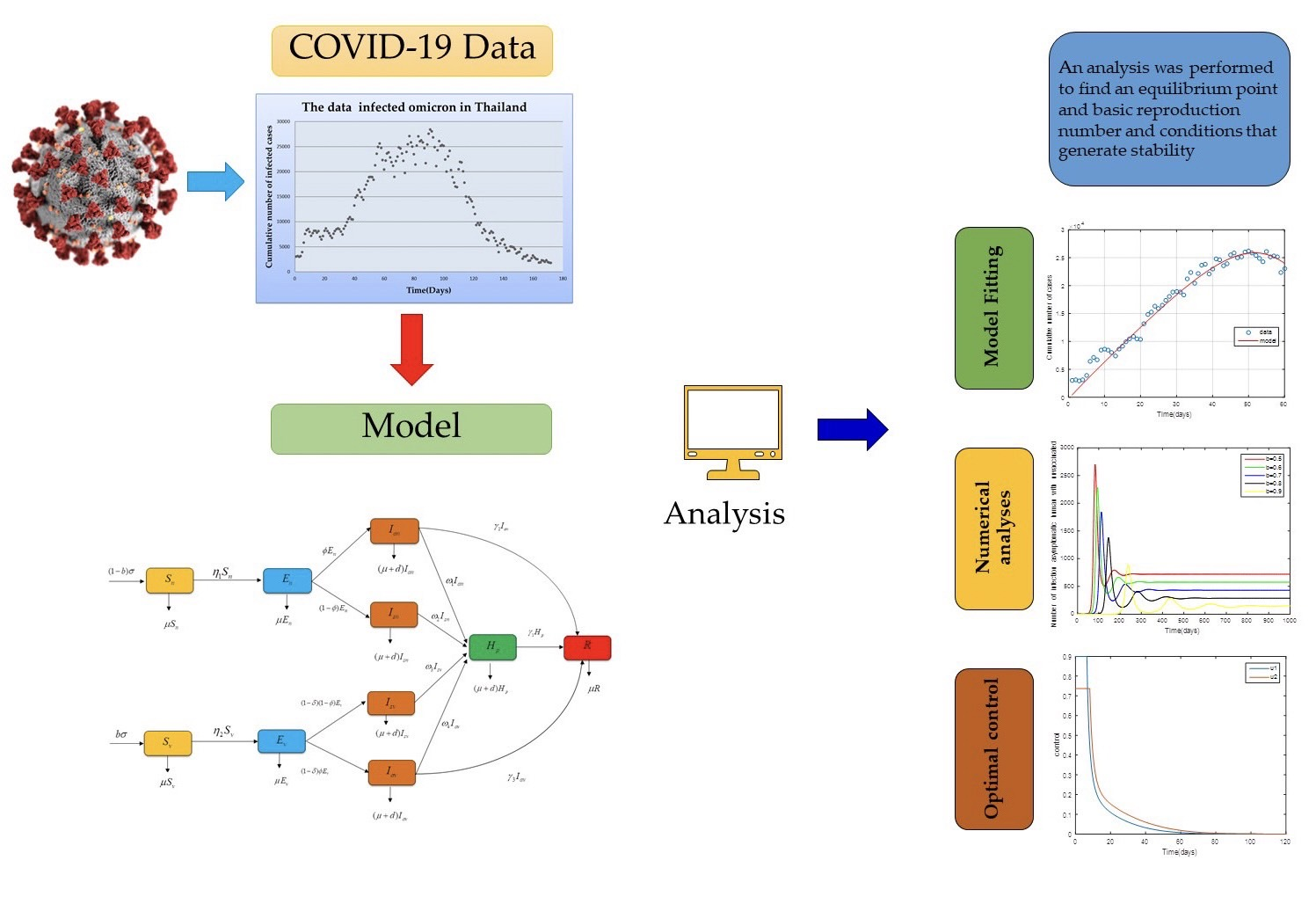
Vaccination’s Role in Combating the Omicron Variant Outbreak in Thailand: An Optimal Control Approach

1
Department of Mathematics, School of Science, King Mongkut’s Institute of Technology Ladkrabang, Bangkok 10520, Thailand
2
Department of Physics, Faculty of Science, Mahidol University, Bangkok 10400, Thailand
3
Department of Instrumentation and Control Engineering, School of Engineering, King Mongkut’s Institute of Technology Ladkrabang, Bangkok 10520, Thailand
*
Author to whom correspondence should be addressed.
Mathematics 2022, 10(20), 3899; https://doi.org/10.3390/math10203899
Submission received: 28 September 2022 / Revised: 13 October 2022 / Accepted: 16 October 2022 / Published: 20 October 2022

Abstract

:
COVID-19 is the name of the new infectious disease which has reached the pandemic stage and is named after the coronavirus (COVs) which causes it. COV is a single-stranded RNA virus which in humans leads to respiratory tract symptoms which can lead to death in those with low immunities, particularly older people. In this study, a standard dynamic model for COVID-19 was proposed by comparing a simple model and the optimal control model to reduce the number of infected people and become a guideline to control the outbreak. Control strategies are the vaccination rate and vaccine-induced immunity. An analysis was performed to find an equilibrium point, the basic reproduction number ( R 0 ) , and conditions that generate stability by using Lyapunov functions to prove the stability of the solution at the equilibrium point. Pontryagin’s maximum principle was used to find the optimal control condition. Moreover, sensitivity analysis of the parameters was performed to learn about the parameters that might affect the outbreak in order to be able to control the outbreak. According to the analysis, it is seen that the efficacy of vaccines ( b ) and the infection rate ( β a n , β s n , β a v , β s v ) will affect the increased (decreased) incidence of the outbreak. Numerical analyses were performed on the Omicron variant outbreak data collected from the Thailand Ministry of Health, whose analyses then indicated that the optimal control strategy could lead to planning management and policy setting to control the COVID-19 outbreak.

Graphical Abstract

1. Introduction

A huge outbreak of COVID-19 infections has reached every corner of the world. It is now considered to be the largest health threat to the world since there are now millions of confirmed cases of infection. Due to the pathogens of the COVID-19 virus, a single-stranded RNA virus [1] belonging to the family of Coronaviridae, it causes respiratory sickness. The coronaviruses can be classified into at least four genera: Alphacoronavirus, Betacoronavirus, Gammacoronavirus and Deltacoronavirus. The coronaviruses that cause diseases in humans but do not cause severe respiratory symptoms or asymptomatic syndrome are members of the Alphacoronavirus genus. The coronaviruses that cause severe diseases in humans such as severe acute respiratory syndrome (SARS) and Middle East respiratory syndrome (MERS), SARS-CoV and MERS-CoV, belong to the Betacoronavirus genus. These last two viruses originated in animals but have crossed the species (animal-to-human) barrier. The new coronaviruses in 2019 are a family of viruses which cause illnesses ranging from the common cold to more severe diseases [2,3] and appeared only recently in humans. They first appeared in bats. In humans, these viruses cause respiratory illnesses.
COVID-19 is transmitted from person to person [4,5] through the air by droplets of liquid that come from the noses and mouths of infected people when they cough, sneeze, and talk, or by touching surfaces that are contaminated with the virus [6]. The length of time between infection and the appearance of the first symptoms (incubation period) is between 1 and 14 days (5–6 days on average). More than 97% of patients begin to show symptoms of illness within 14 days. General symptoms include fever, fatigue, headache, runny nose, sore throat, coughing, rapid breathing, and difficulty breathing. In severe cases, patients may begin to show complications such as pneumonia, lung inflammation, renal failure, or death [2,4,5,7,8]. Currently, there is no clear information showing how long COVID-19 can survive on surfaces. It was found that viruses would not survive after being exposed to disinfectants [8].
The spread of COVID-19 was first reported in the city of Wuhan in China when it originated that a continuously increasing number of patients having pneumonia of unknown etiology began in December 2019. It was officially reported on 3 January 2020 that the pneumonia outbreak in Wuhan was caused by a new coronavirus (novel coronavirus 2019, 2019-nCoV) [5,9,10,11,12,13] through person-to-person contact. On 22 January 2020, the Thailand Department of Disease Control, Ministry of Public Health elevated the emergency operations to be level 3 (avoiding traveling). The Ministry of Public Health implemented measures for temperature monitoring and screening at immigration checkpoints to monitor and detect travelers at risk of COVID-19 infection. As of 29 June 2022, Thailand has reported a cumulative total of 4,520,220 confirmed cases with 30,634 deaths [14]. Unlike many countries in the world, Thailand has a well-developed public health system with free medical health centers in every part of the country. The health centers are staffed by medical doctors and nurses who are governmental employees working to serve the people. Nothing is preventing Thailand from controlling the COVID-19 pandemic except for the lack of knowledge on the spread of the disease, the control steps tailored to the country, and the vaccines needed for preventing the spread of the virus. This study aims to provide the knowledge needed to efficiently control the spread of the disease.
Mathematical modeling is a tool for analyzing strategies needed to control the spread of COVID-19. From past to present, numerous researchers have proposed different models of the spread of COVID-19 needed to study the dynamic of the spread. In the first half of the 20th century, the SEIR model was used to understand the behavior of infectious diseases, with many researchers incorporating its use in developing the relevant mathematical models to predict transmission dynamics with a view to control [15]. These have included well known epidemics such as MERS [16], influenza [17,18,19], and dengue fever [20,21]. Gardner, Rey, et al. [22] introduced a basic model to study the spread of MERS-CoV in the Arabian Peninsula, Europe, North America, Southeast Asia, the Middle East, and the United States of America. The spread of MERS-CoV is not exactly the same as that of severe acute respiratory syndrome SARS-CoV. Both of these coronaviruses are transmitted by person-to-person contact. Differences in the epidemiology are used to create the mathematical model for each coronavirus. The differences in the MERS-CoV transmission were the locations of the contact and who the human contacts were. Ndaïroua et al. [11] created a mathematical model to study the spread of COVID-19 in Wuhan, China. How humans get infected was studied, and from this, the basic reproduction number was calculated, while sensitivity of the parameters affecting the spread was considered. Enahoro et al. [10] developed a mathematical model to study the dynamic of the spread and control of COVID-19 in Nigeria. The model analyzed and determined the parameters using COVID-19 information publicized by the Nigeria Center of Disease Control (NCDC) to assess the effects across the country and within communities. Numerical simulation in the mathematical model showed that COVID-19 could be efficiently controlled in Nigeria by using a moderate level of social distancing across the country. Sen [23] created a mathematical model for the spread of COVID-19 in the form of the SEIRD model (susceptible–infected–recovered–dead model) by analyzing the spread in five countries, i.e., China, Italy, France, United States of America, and India. Curve fitting analysis was conducted to compare the spread between real information and the created model. Kumar et al. [24] developed a simple mathematical model to predict and examine the spread of COVID-19 in India. A mathematical method was proposed to predict new cases of COVID-19 or cumulative confirmed cases in real situations. Various simulation models were presented to predict the spread of COVID-19 in India and other countries. Hezam et al. [25] proposed a dynamic mathematical model to control the spread of COVID-19 and cholera in Yemen. All four control functions were used, namely, social distancing, lockdown, number of tests, and number of chlorine tablets. Riyapan et al. [26] created a mathematical model and conducted an analysis to understand the dynamic of COVID-19 spread in Bangkok. People were divided into seven groups, i.e., susceptible group, exposed group, infected group, asymptomatic group, symptomatic group (quarantined), recovered group, and dead group. According to the model analysis and numerical results, it was shown that wearing a mask regularly could reduce the spread of COVID-19.
From what was mentioned earlier, it can be seen that this research is different from the research studies mentioned above. The objective of this research is to analyze the dynamic of COVID-19 by creating a mathematical model, and consideration is made when people get vaccinated for COVID-19. Specifically, the infective individuals’ trajectories with several values of vaccination efficacies are compared against one another to see the effects that the efficacies have on these trajectories. Furthermore, a numerical analysis is also conducted on the infective data collected from the Thai Ministry of Health for the Omicron variant outbreak, whereby the rates of transmission of symptomatic and asymptomatic infections are estimated. Optimal control analyses are then performed to compare its effectiveness against the uncontrolled counterparts. It is seen that the controlled trajectories outperform the uncontrolled counterparts.

2. Materials and Methods

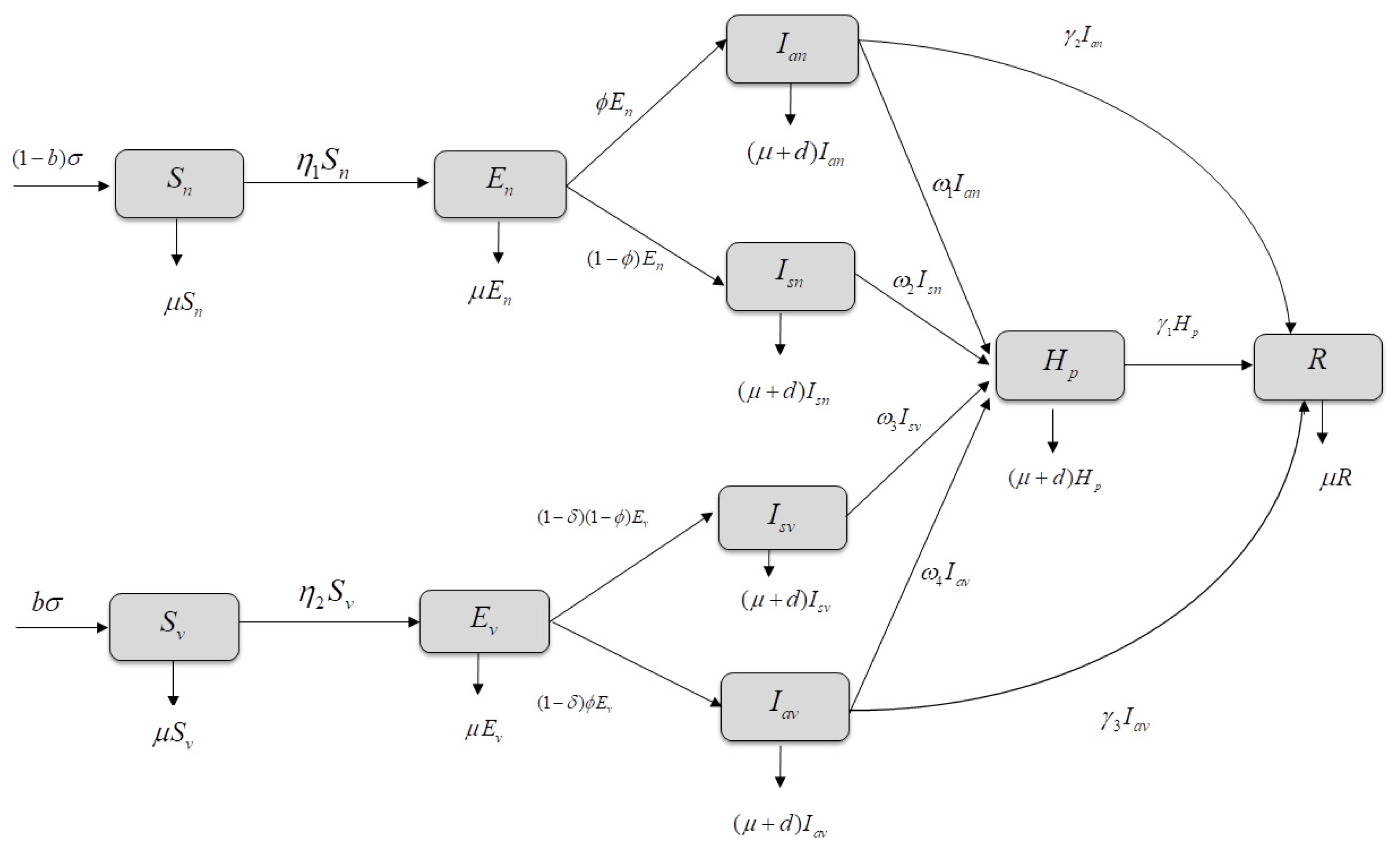
2.1. Mathematical Model

Yang and Wang [7] proposed a COVID-19 mathematical model in the form of the SEIHRV model (susceptible–exposed–infected–hospitalized–recovered model) to study the spread of COVID-19 by comparing different infection rates based on the Hamilton County (USA) case reports. The study found that environmental factors played an important role in the spread of COVID-19. Rajputet al. [27] proposed a nonlinear mathematical model as a strategy for controlling the spread of COVID-19 by using vaccination as a means to reduce the infection. Both studies are consistent with and are similar to the research here. The World Health Organization (WHO) has reported that people vaccinated against COVID-19 with one of the approved COVID-19 vaccines develop illnesses of different severity, i.e., the symptoms of patients whose infectious status are due to the exposure to mRNA fragments in the vaccine could be mild or strong enough to prevent hospitalization, depending on the immune status of the patient and which vaccine was used. It should be noted that the vaccines are only approved for different age groups. In order to be able to take into account the possibility of the responses of individuals to the exposure to mRNA of COVID-19 in its natural state or the mRNA in the vaccine, a modification of the population groups in the model is made. In this research, the population is first divided into two groups, the vaccinated population and the unvaccinated population, to study differences in the responses of both groups. In addition, each population is further divided into subgroups as follows: a group labelled unvaccinated and the susceptible population, a group of unvaccinated and the exposed population, a group of unvaccinated and the asymptomatic population, a group of unvaccinated and the symptomatic population, a group of vaccinated and the susceptible population, a group of vaccinated and the exposed population, a group of vaccinated and the asymptomatic population, a group of vaccinated and the symptomatic population, a group of the hospitalized population, and a group of the recovered population. Note that the isolated infected population group is not explicitly included in the model but is rather included in the symptomatic infectious group. This is because there was already a widespread use of the antigen testing kit amongst the Thai population, even in the rural regions, by the time of the Omicron outbreak; the symptomatic infectious population, upon testing positive for COVID-19 with the kit, automatically isolated themselves and received appropriate treatments via post mails. The developed model is then dynamically analyzed to investigate the appropriate control measures.
The transmission dynamics are encapsulated in the following diagram.
Susceptible groups for the unvaccinated population infected with COVID-19 have the rates of β a n   and   β s n . The infection rate of the unvaccinated population η 1 is determined as:
η 1 = β a n I a n + β s n I s n
Similarly, the infection rate of the vaccinated population η 2 is determined as:
η 2 = β a v I a v + β s v I s v
From the diagram in Figure 1, the infection dynamics can be described as follows:
The initial number in the unvaccinated human population susceptible to COVID-19 is ( 1 b ) σ when 0 < b < 1 . The unvaccinated and infected human population will transmit the virus to the susceptible human population with the probabilities of β a n   and   β s n , respectively. When the human population is exposed to COVID-19, the incubation period is at the rate of ϕ . If the body’s immune response is absent, they become infected. Infection in humans can be symptomatic, showing symptoms, or asymptomatic, both being infectious (able to transmit the infection). After getting infected, infected persons shall be hospitalized with the rate of ω 1   and   ω 2 , respectively. When infected with COVID-19, some people die of the disease, with a death rate of d . However, infected people who are asymptomatic may not be hospitalized. After undergoing COVID-19 treatment, infected people will recover. The human population shall die of natural causes at a rate of μ .
The number in the vaccinated human population susceptible to COVID-19 is b σ . The vaccinated and infected human population shall transmit the virus to the susceptible human population with the probability of β a v   and   β s v , respectively. When the human population is exposed to COVID-19, the incubation period is at the rate of ( 1 δ ) . If the body’s immune response is absent, they become infected. Infection in humans is divided into 2 characteristics, namely, symptomatic infection and asymptomatic infection. After getting infected, infected persons shall be hospitalized with the rate of   ω 3   and   ω 4 , respectively. When infected with COVID-19, some people die of the disease, with a death rate of d . Most of the infected people who are asymptomatic may not be hospitalized. After undergoing COVID-19 treatment, infected people will recover. The human population shall die of natural causes at a rate of μ .
A model of COVID-19 and vaccinations can be created by describing the relationship of the mathematical model as follows:
d S n d t = ( 1 b ) σ η 1 S n μ S n
d E n d t = η 1 S n ϕ E n ( 1 ϕ ) E n μ E n
d I a n d t = ϕ E n ( ω 1 + γ 2 + μ + d ) I a n
d I s n d t = ( 1 ϕ ) E n ( ω 2 + μ + d ) I s n
d S v d t = b σ η 2 S v μ S v
d E v d t = η 2 S v ( 1 δ ) ϕ E v ( 1 δ ) ( 1 ϕ ) E v μ E v
d I a v d t = ( 1 δ ) ϕ E v ( ω 4 + γ 3 + μ + d ) I a v
d I a v d t = ( 1 δ ) ( 1 ϕ ) E v ( ω 3 + μ + d ) I s v
d H p d t = ω 1 I a n + ω 2 I s v + ω 3 I s v + ω 4 I a v ( γ 1 + μ + d ) H p
d R d t = γ 1 H p + γ 2 I a n + γ 3 I a v μ R
when
N h = S n + E n + I a n + I s n + S v + E v + I a v + I s v + H p + R
where the parameters of Equations (3)–(12) are defined in Table 1.
Lemma 1.
(From [28,29]). Let ( S n ( t ) , E n ( t ) , I a n ( t ) , I s n ( t ) , S v ( t ) , E v ( t ) , I a v ( t ) , I s v ( t ) , H p ( t ) , R ( t ) ) be the solution of the system (3)–(12) with positive initial conditions S n ( 0 ) , E n ( 0 ) , I a n ( 0 ) , I s n ( 0 ) ,   S v ( 0 ) , E v ( 0 ) , I a v ( 0 ) , I s v ( 0 ) , H p ( 0 ) , R ( 0 ) . Denoting also the invariant set
Ω = { ( S n , E n , I a n , I s n , S v , E v , I a v , I s v , H p , R R 10 + : N h σ μ } , and Ω is a positively invariant set for (3)(12).
Proof. 
Where N h = S n + E n + I a n + I s n + S v + E v + I a v + I s v + H p + R , the formula will be:
d N h d t = d S n d t + d E n d t + d I a n d t + d I s n d t + d S v d t + d E v d t + d I a v d t + d I s v d t + d H p d t + d R d t d N h d t = d S n d t σ μ N h d ( I a n + I s n + I a v + I s v + H p )      σ μ N h
It can be seen that d N h d t σ μ N h 0 . Therefore, when N h ( t ) N ( 0 ) e μ t + σ μ [ 1 e μ t ] , the derivative   d N h d t satisfies d N h d t σ μ . Hence, as t , e μ t 0 , it then follows that all trajectories within the invariant set   Ω will form a positively invariant set in R 10 + for the systems (3)–(12) since all epidemiological constants are nonnegative. □

2.2. Stability Analysis

2.2.1. Equilibrium Point

The dynamical systems analysis for the models of (3)–(12) can be performed, firstly, by evaluating the equilibrium of the system. This is conducted by setting Equations (3)–(12) to zero. The two such equilibrium points for this system are as follows:
The disease-free equilibrium point is:
G 0 * = ( S n * , E n * , I a n * , I s n * , S v * , E v * , I a v * , I s v * , H p * , R * ) = ( ( 1 b ) σ μ , 0 , 0 , 0 , b σ μ , 0 , 0 , 0 , 0 , 0 )
when R 0 < 1 , and the endemic equilibrium point is:
G 1 * = ( S n * , E n * , I a n * , I s n * , S v * , E v * , I a v * , I s v * , H p * , R * )
when
S n * = ( 1 b ) σ ( μ + η 1 * ) , E n * = ( 1 b ) σ η 1 * ( 1 + μ ) ( μ + η 1 * ) , I a n * = ( 1 b ) ϕ σ η 1 * k 1 , I s n * = ( 1 b ) ( 1 ϕ ) σ η 1 * k 2 , S v * = b σ ( μ + η 2 * ) , E v * = b σ η 2 * ( 1 + μ δ ) ( μ + η 2 * ) , I a v * = b ( 1 δ ) ϕ σ η 2 * ( 1 + μ δ ) k 3 , I s v * = b ( 1 δ ) ( 1 ϕ ) σ η 2 * ( 1 + μ δ ) k 4 ,
H p * = k 5 ( ( 1 b ) ϕ ω 1 η 1 * k 1 + ( 1 b ) ( 1 ϕ ) ω 2 η 1 * k 2 + b ( 1 δ ) ϕ ω 4 η 2 * ( 1 + μ δ ) k 3 + b ( 1 δ ) ( 1 ϕ ) ω 3 η 2 * ( 1 + μ δ ) k 4 )
R * = k 6 ( ( 1 b ) ϕ γ 2 η 1 * k 1 + b ( 1 δ ) ϕ γ 3 η 2 * ( 1 + μ δ ) k 3 + k 7 ( ( 1 b ) ϕ ω 1 η 1 * k 1 + ( 1 b ) ( 1 ϕ ) ω 2 η 1 * k 2 + b ( 1 δ ) ϕ ω 4 η 2 * ( 1 + μ δ ) k 3 + b ( 1 δ ) ( 1 ϕ ) ω 3 η 2 * ( 1 + μ δ ) k 4 ) )
where k 1 = ( 1 + μ ) ( d + γ 2 + μ + ω 1 ) ( μ + η 1 * ) ,   k 2 = ( 1 + μ ) ( d + μ + ω 2 ) ( μ + η 1 * ) ,   k 3 = ( d + γ 3 + μ + ω 4 ) ( μ + η 2 * ) ,   k 4 = ( d + μ + ω 3 ) ( μ + η 2 * ) , and k 5 = σ γ 1 + μ + d ,   k 6 = σ μ ,   k 5 = γ 1 γ 1 + μ + d , when R 0 > 1 .
The forces of infection, η 1 *   and   η 2 * , appearing in the components of the endemic equilibrium point can be determined by using the following expressions:
η 1 * = β a n I a n * + β s n I s n *
and
η 2 * = β a v I a v * + β s v I s v *

2.2.2. The Basic Reproduction Number

The calculation of the basic reproduction number ( R 0 ) plays a huge and important role since it is used to measure the transmission potential of a disease. It is the average number of secondary infections which can be caused by a patient in a completely susceptible population throughout this infectious period. In this research, the basic reproduction number was calculated using the next-generation matrix method [30,31] for COVID-19 mathematical model. The states E n , I a n , I s n , E v , I a v and I s v were chosen to construct the gain and loss vectors, where the gain vector represents the possible pathways of creating new infections, and the loss vector represents the possible pathways of transferring from one group to another.
| G a i n s   t o   E n G a i n s   t o   I a n G a i n s   t o   I s n G a i n s   t o   E v G a i n s   t o   I a v G a i n s   t o   I s v | | η 1 S n 0 0 η 2 S v 0 0 | ,   | L o s s e s   f r o m   E n L o s s e s   f r o m   I a n L o s s e s   f r o m   I s n L o s s e s   f r o m   E v L o s s e s   f r o m   I a v L o s s e s   f r o m   I s v | | ϕ E n + ( 1 ϕ ) E n + μ E n ϕ E n + ( ω 1 + γ 2 + μ + d ) I a n ( 1 ϕ ) E n + ( ω 2 + μ + d ) I s n ( 1 δ ) ϕ E v + ( 1 δ ) ( 1 ϕ ) E v + μ E v ( 1 δ ) ϕ E v + ( ω 4 + γ 3 + μ + d ) I a v ( 1 δ ) ( 1 ϕ ) E v + ( ω 3 + μ + d ) I s v |
The required F and V matrices are the Jacobian matrices of the gain and loss vectors, respectively. Then we have
F = [ 0 β a n S n β s n S n 0 0 0 0 0 0 0 0 0 0 0 0 0 0 0 0 0 0 0 β a v S v β s v S v 0 0 0 0 0 0 0 0 0 0 0 0 ]
V = [ ϕ + ( 1 ϕ ) + μ 0 0 0 0 0 ϕ ω 1 + μ + d 0 0 0 0 ( 1 ϕ ) 0 ω 2 + μ + d 0 0 0 0 0 0 ( 1 δ ) ϕ + ( 1 δ ) ( 1 ϕ ) + μ 0 0 0 0 0 ( 1 δ ) ϕ ω 4 + γ 3 + μ + d 0 0 0 0 ( 1 δ ) ( 1 ϕ ) 0 ω 3 + μ + d ]
Note that we evaluate the gain and loss matrices at the disease-free equilibrium point:
G 0 * = ( S n * , E n * , I a n * , I s n * , S v * , E v * , I a v * , I s v * , H p * , R * ) = ( ( 1 b ) σ μ , 0 , 0 , 0 , b σ μ , 0 , 0 , 0 , 0 , 0 )
The required basic reproduction number is computed as R 0 = F V 1 , where R 0   is the maximum positive eigenvalue of the matrix F V 1 . Therefore, the formula is:
R 0 = m a x { R n , R v }
when
R n = ( b 1 ) σ ( d ( β s n ( ϕ 1 ) β a n ϕ ) + β s n ( ϕ 1 ) ( γ 2 + μ + ω 1 ) β a n ϕ ( μ + ω 2 ) μ ( 1 + μ ) ( d + γ 2 + μ + ω 1 ) ( d + μ + ω 2 ) R v = b σ ( δ 1 ) ( d ( β s v ( ϕ 1 ) β a v ϕ ) β a v ϕ ( μ + ω 3 ) β s v ( ϕ 1 ) ( γ 3 + μ + ω 4 ) μ ( 1 δ + μ ) ( d + μ + ω 3 ) ( d + γ 3 + μ + ω 4 )

2.2.3. Global Stability Analysis

In this part, the global stability analysis of each equilibrium point of the model in the system of Equations (3)–(12) around the two steady states G 0 * and G 1 *   is performed as demonstrated in the following.
Theorem 1.
The disease-free equilibrium point G 0 * of the model in the system (3)(12) is globally asymptotically stable in Ω if R 0 < 1 .
We assume that
{ β a n = β s n = μ + d S n * β a v = β s v = μ + d S v *
Proof. 
Consider the continuously differentiable linear Lyapunov function defined by
L = ( S n S n * l n S n ) + E n + I a n + I s n + ( S v S v * l n S v ) + E v + I a v + I s v + H p + R
To explain the use of l n S n and l n S v have
d L d t = S n ( 1 S n * S n ) + E n + I a n + I s n + S v ( 1 S v * S v ) + E v + I a v + I s v + H p + R
d L d t = ( ( 1 b ) σ η 1 S n μ S n ) ( 1 S n * S n ) + ( η 1 S n ϕ E n ( 1 ϕ ) E n μ E n ) + ( ϕ E n ( ω 1 + γ 2 + μ + d ) I a n ) + ( ( 1 ϕ ) E n ( ω 2 + μ + d ) I s n ) + ( b σ η 2 S v μ S v ) ( 1 S v * S v ) + ( η 2 S v ( 1 δ ) ϕ E v ( 1 δ ) ( 1 ϕ ) E v μ E v ) + ( ( 1 δ ) ϕ E v ( ω 4 + γ 3 + μ + d ) I a v ) + ( ( 1 δ ) ( 1 ϕ ) E v ( ω 3 + μ + d ) I s v ) + ( ω 1 I a n + ω 2 I s v + ω 3 I s v + ω 4 I a v ( γ 1 + μ + d ) H p ) + ( γ 1 H p + γ 2 I a n + γ 3 I a v μ R )    = ( 1 b ) σ ( 1 S n * S n ) + β a n I a n S n * + β s n I s n S n * μ S n + μ S n * μ E n ( μ + d ) I a n ( μ + d ) I s n + b σ ( 1 S v * S v ) + β a v I a v S v * + β s v I s v S v * μ S v + μ S v * μ E v ( μ + d ) I a v ( μ + d ) I s v ( μ + d ) H p μ R    = ( 1 b ) σ ( 1 S n * S n ) + μ S n * ( 1 S n S n * ) + ( β a n S n * ( μ + d ) ) I a n + ( β s n S n * ( μ + d ) ) I s n μ E n + b σ ( 1 S v * S v ) + μ S v * ( 1 S v S v * ) + ( β a v S v * ( μ + d ) ) I a v + ( β s v S v * ( μ + d ) ) I s v μ E v ( μ + d ) H p μ R
Substitute Equation (19) to obtain
d L d t = ( 1 b ) σ ( 1 S n * S n ) + μ S n * ( 1 S n S n * ) μ E n + b σ ( 1 S v * S v ) + μ S v * ( 1 S v S v * ) μ E v ( μ + d ) H p μ R
Substitute S n * = ( 1 b ) σ μ and S v * = b σ μ from the disease-free equilibrium point to obtain
d L d t = ( 1 b ) σ ( 1 S n * S n ) + μ ( 1 b ) σ μ   ( 1 S n S n * ) + b σ ( 1 S v * S v ) + μ b σ μ ( 1 S v S v * ) μ E n ( μ + d ) H p μ R
d L d t = ( 1 b ) σ ( 1 S n * S n ) + ( 1 b ) σ ( 1 S n S n * ) + b σ ( 1 S v * S v ) + b σ ( 1 S v S v * ) μ E n ( μ + d ) H p μ R = ( 1 b ) σ ( 2 S n * S n S n S n * ) + b σ ( 2 S v * S v S v S v * ) μ E n ( μ + d ) H p μ R = ( 1 b ) σ ( ( S n * S n ) 2 S n * S n ) b σ ( ( S v * S v ) 2 S v * S v ) μ E n ( μ + d ) H p μ R
d L d t = [ ( 1 b ) σ ( ( S n * S n ) 2 S n * S n ) + b σ ( ( S v * S v ) 2 S v * S v ) + μ E n + ( μ + d ) H p + μ R ] 0
It can be clearly seen that all conditions shown in Equation (20) are negative. Applying the LaSalle’s invariance principle [4,32,33,34], d L d t = 0 if S n * = S n   and   S v * = S v , and 1 b is a positive number since it is known that 0 < b < 1 . Note further that, d L d t = 0   if E n = 0   E v = 0 ,   H p = 0   and   R = 0 . On the other hand, the result of Theorem 1 implies that since the states E n , E v ,   H p , and R are all positive, the resulting d L d t obtained in Equation (20) will be absolute negative. Consequently, LaSalle’s invariant principle then implies that the disease-free steady state G 0 * is globally asymptotically stable on Ω . □
Theorem 2. 
The endemic equilibrium point G 1 * of the model in the system (3)(12) is globally asymptotically stable in Ω if R 0 > 1 .  We assume that
{ η 1 *   = η 2 * μ     = ( μ + η 1 * ) β s n = ω 2 + μ + d S n *     β s v = ω 3 + μ + d S v *         β s n = ω 2 + μ + d S n *       β a v = ω 4 + γ 3 + μ + d S v *
Proof. 
We consider the following Lyapunov function:
K = ( S n S n * l n S n ) + E n + I a n + I s n + ( S v S v * l n S v ) + E v + I a v + I s v d K d t = S n ( 1 S n * S n ) + E n + I a n + I s n + S v ( 1 S v * S v ) + E v + I a v + I s v
d K d t = ( ( 1 b ) σ η 1 S n μ S n ) ( 1 S n * S n ) + ( η 1 S n ϕ E n ( 1 ϕ ) E n μ E n ) + ( ϕ E n ( ω 1 + γ 2 + μ + d ) I a n ) + ( ( 1 ϕ ) E n ( ω 2 + μ + d ) I s n ) + ( b σ η 2 S v μ S v ) ( 1 S v * S v ) + ( η 2 S v ( 1 δ ) ϕ E v ( 1 δ ) ( 1 ϕ ) E v μ E v ) + ( ( 1 δ ) ϕ E v ( ω 4 + γ 3 + μ + d ) I a v ) + ( ( 1 δ ) ( 1 ϕ ) E v ( ω 3 + μ + d ) I s v ) d K d t = ( 1 b ) σ ( 1 S n * S n ) μ S n ( 1 S n * S n ) + ( β a n I a n + β s n I s n ) S n * μ E n ( ω 1 + γ 2 + μ + d ) I a n ( ω 2 + μ + d ) I s n + b σ ( 1 S v * S v ) μ S v ( 1 S v * S v )          + ( β a v I a v + β s v I s v ) S v * μ E v ( ω 4 + γ 3 + μ + d ) I a v ( ω 3 + μ + d ) I s v     = ( 1 b ) σ ( 1 S n * S n ) + μ S n * ( 1 S n S n * ) + I a n ( ( β a n S n * ( ω 1 + γ 2 + μ + d ) ) + I s n ( β s n S n * ( ω 2 + μ + d ) ) μ E n + b σ ( 1 S v * S v ) + μ S v * ( 1 S v S v * )          + I a v ( β a v S v * ( ω 4 + γ 3 + μ + d ) ) + I s v ( β s v S v * ( ω 3 + μ + d ) ) μ E v
Substitute S n * = ( 1 b ) σ ( μ + η 1 * ) and S v * = b σ ( μ + η 2 * ) from the endemic equilibrium point to obtain
d K d t = ( 1 b ) σ ( 1 S n * S n ) + μ ( 1 b ) σ ( μ + η 1 * ) ( 1 S n S n * ) + I a n ( ( β a n S n * ( ω 1 + γ 2 + μ + d ) ) + I s n ( β s n S n * ( ω 2 + μ + d ) ) μ E n + b σ ( 1 S v * S v ) + μ b σ ( μ + η 2 * ) ( 1 S v S v * ) + I a v ( β a v S v * ( ω 4 + γ 3 + μ + d ) ) + I s v ( β s v S v * ( ω 3 + μ + d ) ) μ E v
Substitute Equation (21) to obtain
d K d t = ( 1 b ) σ ( 1 S n * S n ) + ( 1 b ) σ ( 1 S n S n * ) + b σ ( 1 S v * S v ) + b σ ( 1 S v S v * ) μ E n μ E v = ( 1 b ) σ ( 2 S n * S n S n S n * ) + b σ ( 2 S v * S v S v S v * ) μ E n μ E v = ( 1 b ) σ ( ( S n * S n ) 2 S n * S n ) b σ ( ( S v * S v ) 2 S v * S v ) μ E n μ E v d K d t = [ ( 1 b ) σ ( ( S n * S n ) 2 S n * S n ) + b σ ( ( S v * S v ) 2 S v * S v ) + μ E n + μ E v ] 0
From the condition of Equation (22), d K d t is absolute negative. Then, the endemic equilibrium point G 1 * is globally asymptotically stable in Ω . □

3. Numerical Analysis Result

3.1. Model Fitting

In this part, numerical simulation modelling of the system of Equations (3)–(12) was performed to compare information on the spread in Thailand. Data were collected from COVID-19-infected people from the Department of Disease Control, Ministry of Public Health, Thailand [14] from 1 January 2022, since the Omicron variant was confirmed, until 1 March 2022 to estimate the parameters β a n ,   β s n ,   β a v ,   and   β s v using ode45 and the lsqcurvefit algorithm [12,35] in MATLA,B as shown in Figure 2. Figure 2a depicts the match between the modelled response for the unvaccinated, susceptible individuals against the COVID-19 data. Similarly, Figure 2b then compares the real data against the modelled response for the susceptible, vaccinated individuals. It can be noticed that the simulation model and real information are consistent with one another.

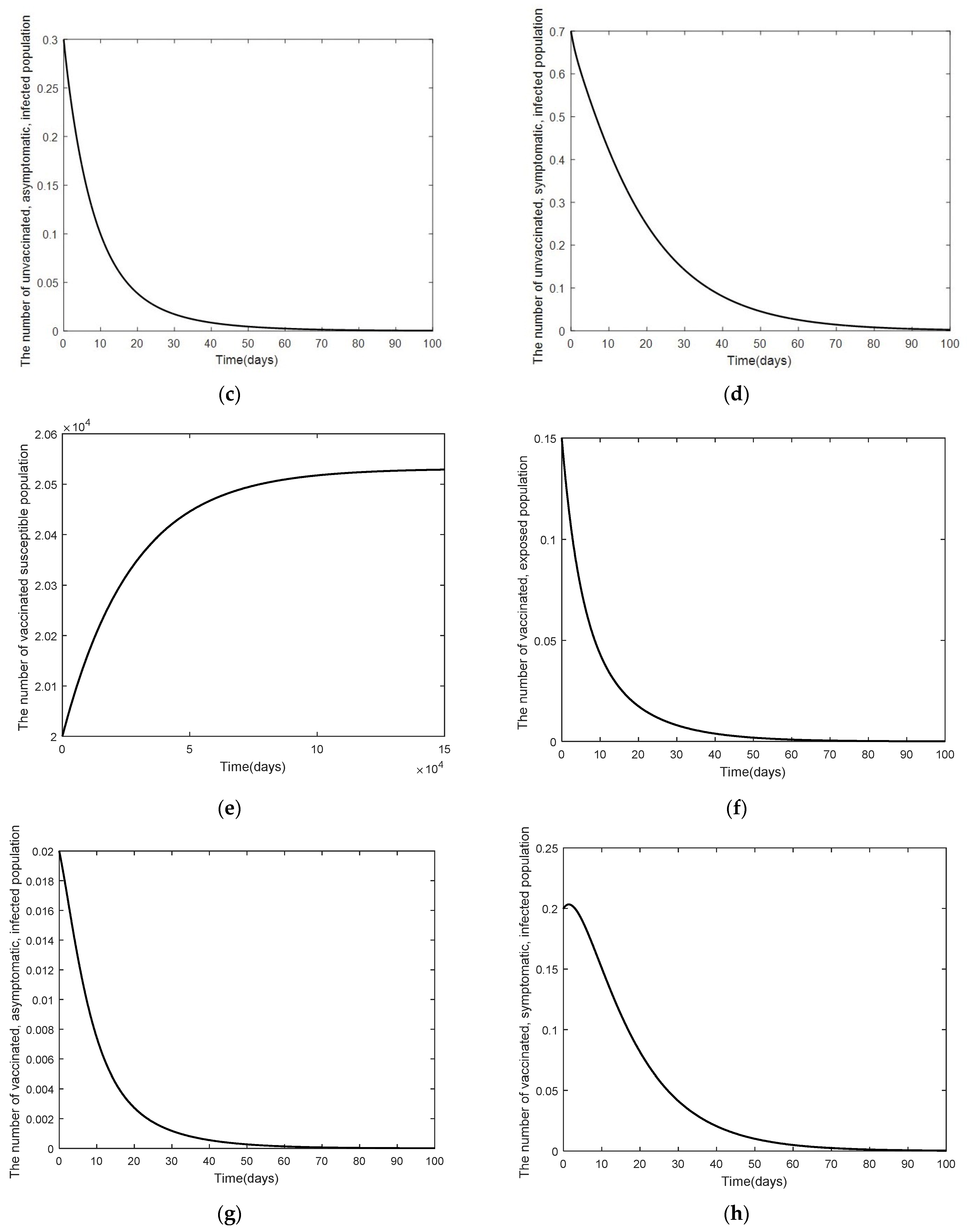
3.2. Numerical Analysis Result

Numerical information on the spread of COVID-19 and getting vaccinations was analyzed using the parameters obtained from the literature review as seen in Table 2 and the data fitted for some parameters, namely, infection rate, β a n ,   β s n ,   β a v ,   and   β s v . The Runge–Kutta method of order 4 in the MATLAB program was used to confirm the equilibrium point result and stability as seen in Figure 3 and Figure 4.
Figure 3 and Figure 4 show the convergence of the number in the unvaccinated, exposed population; the number in the unvaccinated, asymptomatic, infected population; the number in the unvaccinated, symptomatic, infected population; the number in the vaccinated, exposed population; the number in the vaccinated, asymptomatic, infected population; the number in the vaccinated, symptomatic, infected population; the number in the hospitalized population; and the number in the recovered population. It can be noticed that in Figure 3, the graph reached its maximum height and gradually declined to 0, meaning that E n ,   I a n ,   I s n ,   S v ,   E v ,   I a v ,   I s v ,   H p , and   R decreased as time progressed. The number in the unvaccinated, susceptible population and the number in the vaccinated, susceptible population would converge to the equilibrium points of 6849 and 20,547, respectively. This result shows that the states S n   and   S v increase as time increases due to the disease-free steady state when R 0 < 1 . Figure 4 shows the epidemic under the endemic equilibrium point when R 0 > 1 . Note that in this case, the trajectories experience some overshooting at around day 100 before settling down at the equilibrium points.
The World Health Organization defines the efficacy of vaccines as an overall measure of the ability of the vaccine to reduce the chance of getting infected, the death rate, the severity of the illness, the prolonged hospitalization rate, and the ability of the vaccine to creating herd immunity. The efficacy of vaccination depends on numerous factors, such as individual basic health status, individual age when getting the vaccination, or previous exposure to the disease. All factors have effects on the efficacy of vaccines. The effects of the parameters affecting the spread of COVID-19 are shown in Figure 5, Figure 6, Figure 7, Figure 8 and Figure 9. Figure 5 shows the comparison of the efficacy of vaccination by comparing the trajectories for the cases of b = [0.5, 0.6, 0.7, 0.8, 0.9] while keeping the other parameters as given in Table 2. Looking at plots in Figure 5a–d, we see that the graphs overlap. When these graphs are magnified, we see that the number of unvaccinated states, S n ,   E n ,   I a n ,   and   I s n , decrease when the efficacy of the vaccines is increased. Another factor affecting the spread of COVID-19 is the infection rate as seen in Figure 6, Figure 7, Figure 8 and Figure 9. To investigate these cases, we look at the following cases:
  • Case 1: Changes in β a n . Here, the system is simulated with β a n = [0.00001, 0.000034, 0.000054, 0.000074, 0.000094] while keeping the other parameters as given by Table 2.
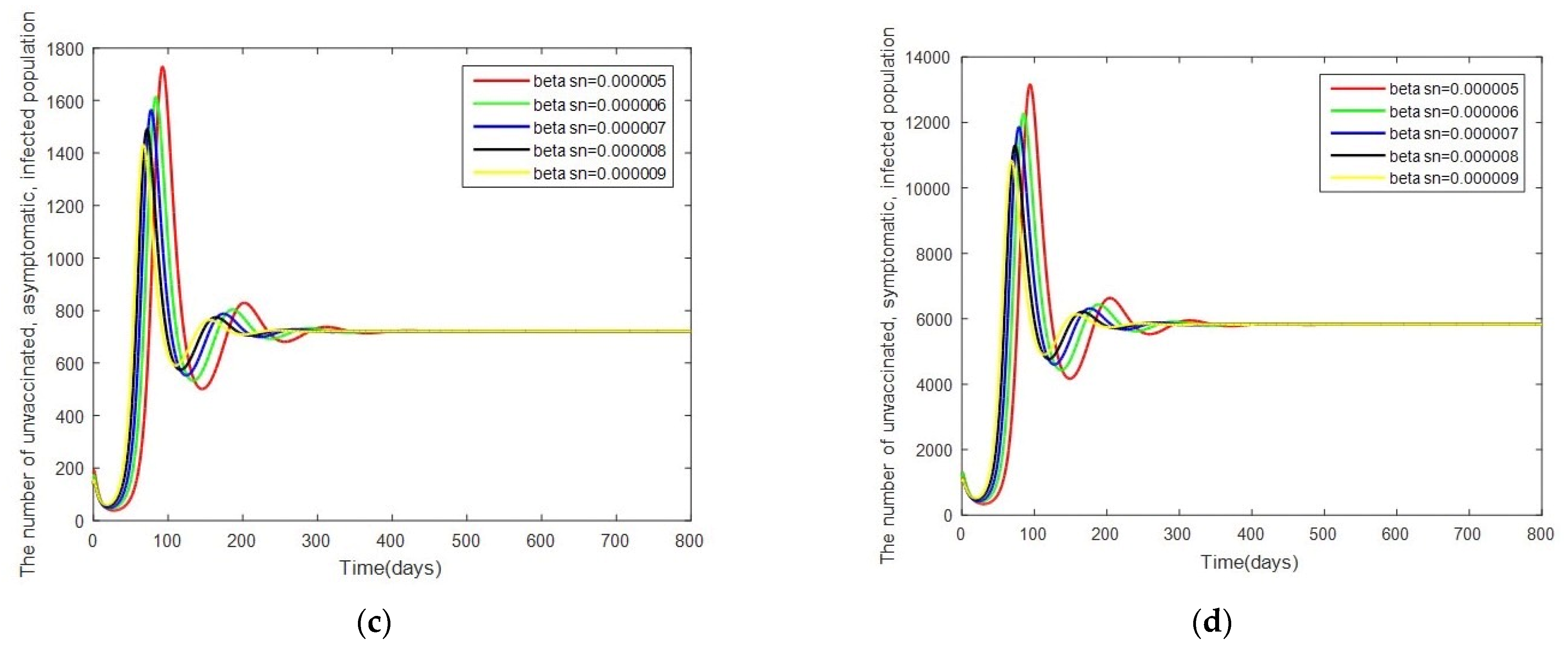
  • Case 2: Changes in β s n . In this case, the system is resimulated with β s n = [0.000005, 0.000006, 0.000007, 0.000008, 0.000009] while keeping the other parameters as given by Table 2.
  • Case 3: Changes in β a v . In this case, the system is resimulated with β a v = [0.000008, 0.00002, 0.00004, 0.00006, 0.00009] while keeping the other parameters as given by Table 2.
  • Case 4: Changes in β s v . In this case, the system is resimulated with β s v = [0.000003, 0.000004, 0.000005, 0.000006, 0.00001] while keeping the other parameters as given by Table 2.
For the susceptible people (both vaccinated and unvaccinated), it is seen from Figure 5, Figure 6, Figure 7, Figure 8 and Figure 9 that a low infection rate causes a slow convergence to an equilibrium point, meaning that disease control will be slower. As for the group of the exposed population, both unvaccinated and vaccinated, exhibiting both symptomatic and asymptomatic symptoms, an infection rate increment causes a quicker convergence to the equilibrium point, contributing to a more rapid onset of disease control. It can be seen that the comparison of the efficacy of vaccination and the infection rate is a better means to control the spread of the disease. To minimize the spread of the disease immediately, everyone needs to strictly follow preventive measures, wear a mask, wash hands thoroughly, and keep social distancing.

3.3. Sensitivity Analysis of Parameters

A sensitivity analysis of the basic reproduction number reveals the parameter values that can affect the numerical simulation model results. In addition, it will indicate the importance of each parameter that affects the basic reproduction number, whose number indicates the spread of the disease. Therefore, a sensitivity analysis of the COVID-19 simulation model from (3)–(12) can provide in-depth information about changes in the spread and can help public health agencies to determine strategies for preventing the spread of COVID-19.
Definition 1.
(Chitnis, Hyman, and Cushing [39]). The normalized forward-sensitivity index of a variable,   R 0 , that depends differentiably on a parameter,   κ , is defined as:
Υ κ R 0 =   R 0 κ × κ R 0
Information in Table 2 is used to show the parameter values for the numerical simulation model. The calculation results of the sensitivity of the basic reproduction number of each parameter are shown in Table 3.
Numerical results from the sensitivity analysis of the basic reproduction number are given in Table 3. If the sensitivity index of the basic reproduction number is positive, it means that an increase (or decrease) in each parameter leads to an increase (or decrease) in the basic reproduction number. Conversely, if the sensitivity index of the basic reproduction number is negative, it means that an increase (or decrease) in each parameter leads to a decrease (or increase) in the basic reproduction number. Consequently, according to the sensitivity analysis of the models (3)–(12), parameters affecting the sensitivity to become positive are b ,   σ ,   β a n ,   β s n ,   β a v ,   β s v ,   and   δ , while parameters affecting the sensitivity to become negative are ϕ ,   ω 1 ,   ω 2 ,   ω 3 ,   ω 4 ,   γ 2 ,   γ 3 ,   μ ,   and   d .
To sum up, the research results indicate that the most effective control strategy is controlling the rate of vaccinated people ( b ) and the initial number of people ( σ ) since the sensitivity index of the parameters is equal to 1. It means that an increase (or decrease) in the rate of vaccinated people, the population birth rate, and the number in the population by 10% enables the basic reproduction number to increase by 10%. The sensitivity analysis mentioned above causes a reduction in the spread of COVID-19 among people in an efficient manner.

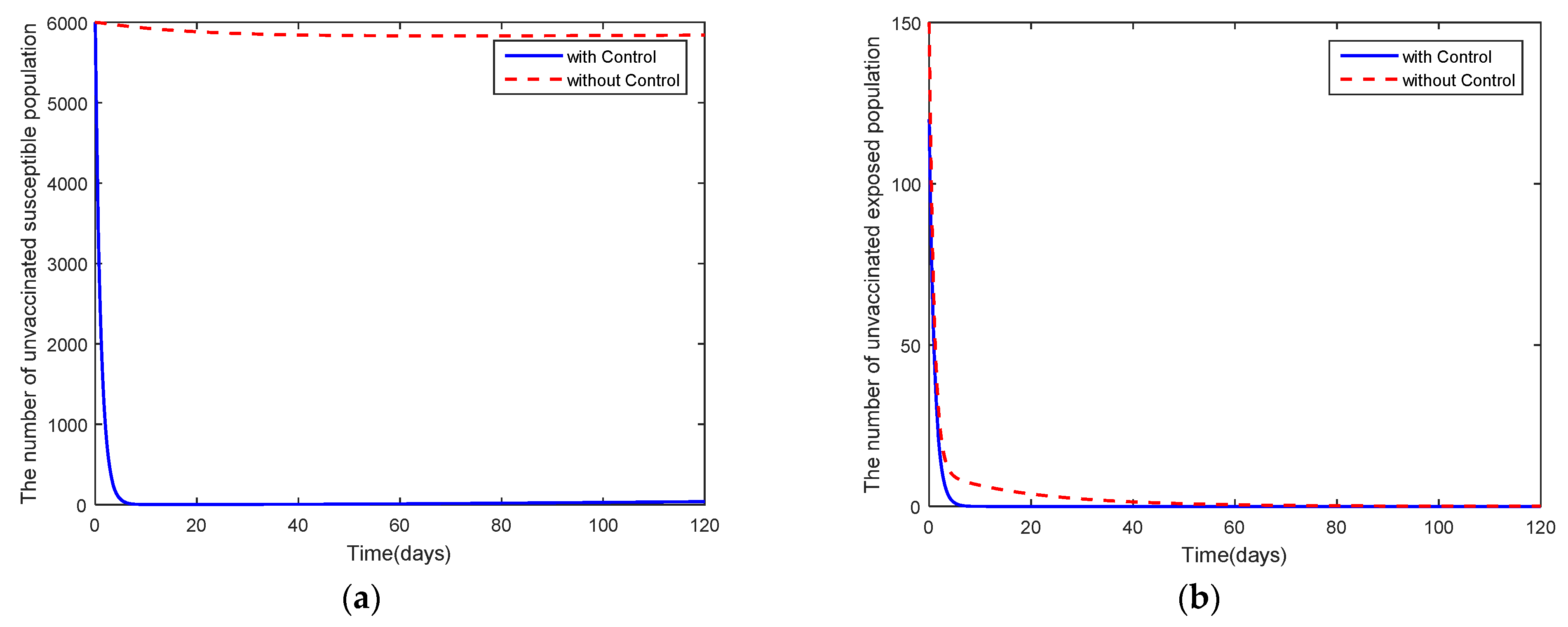
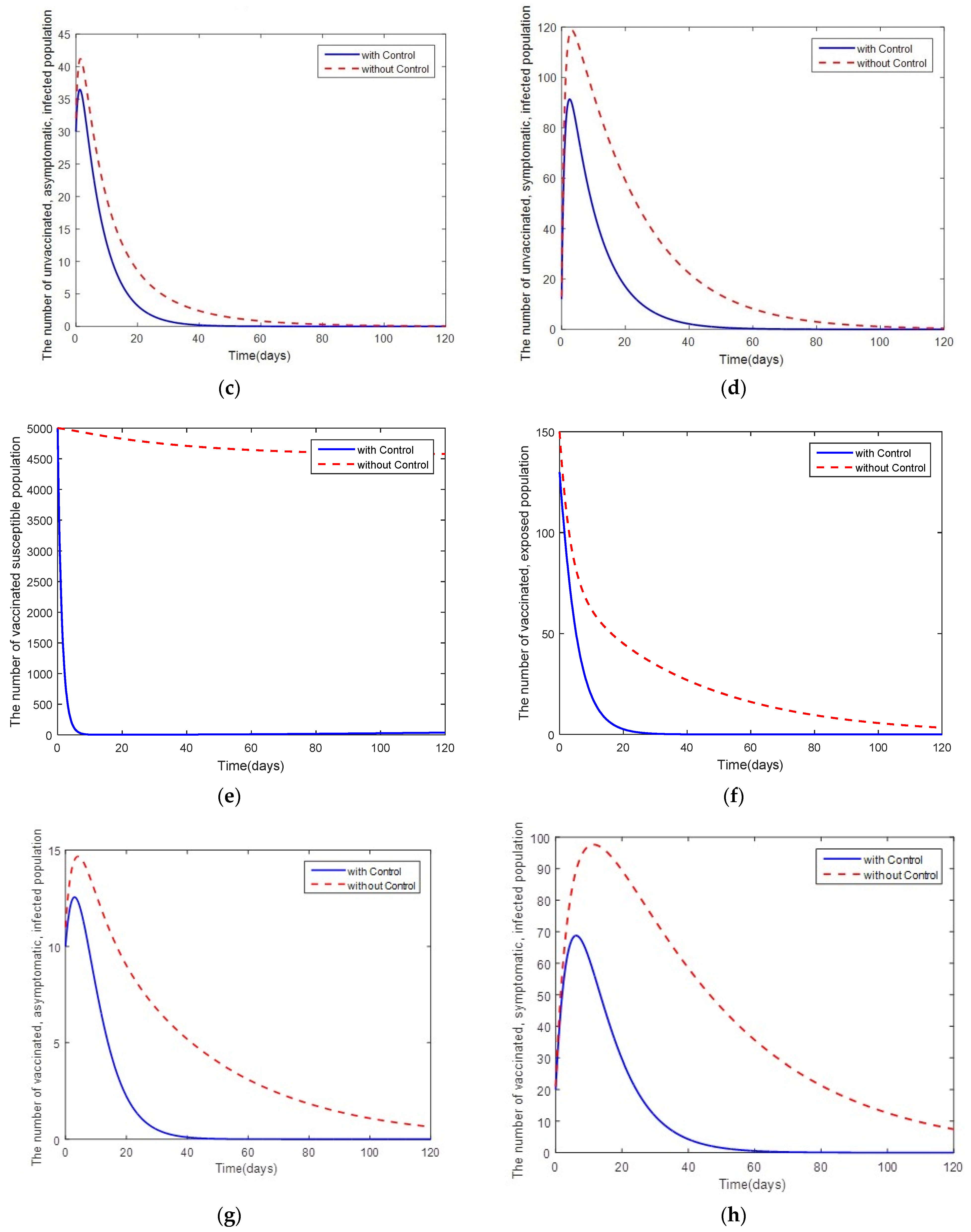
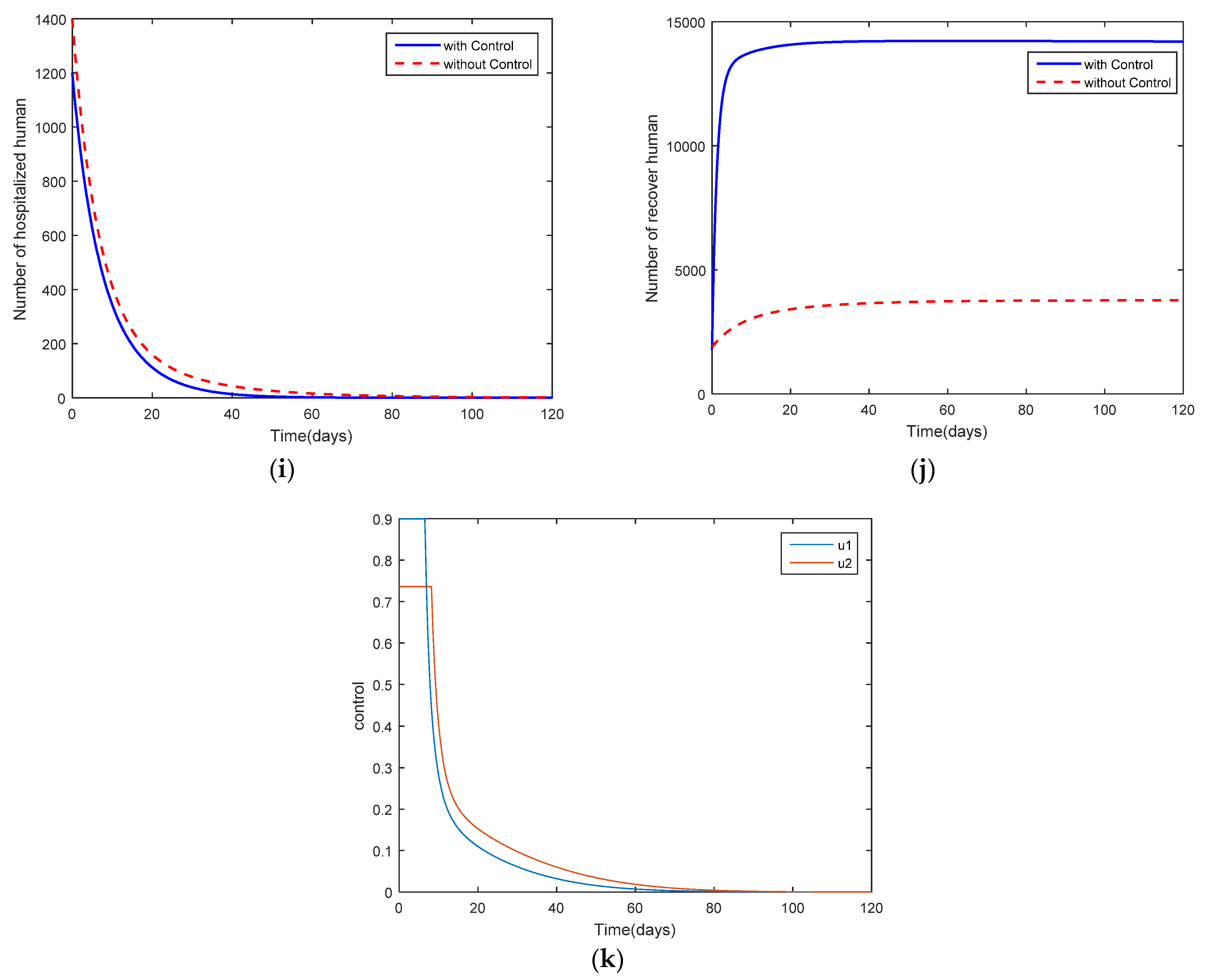
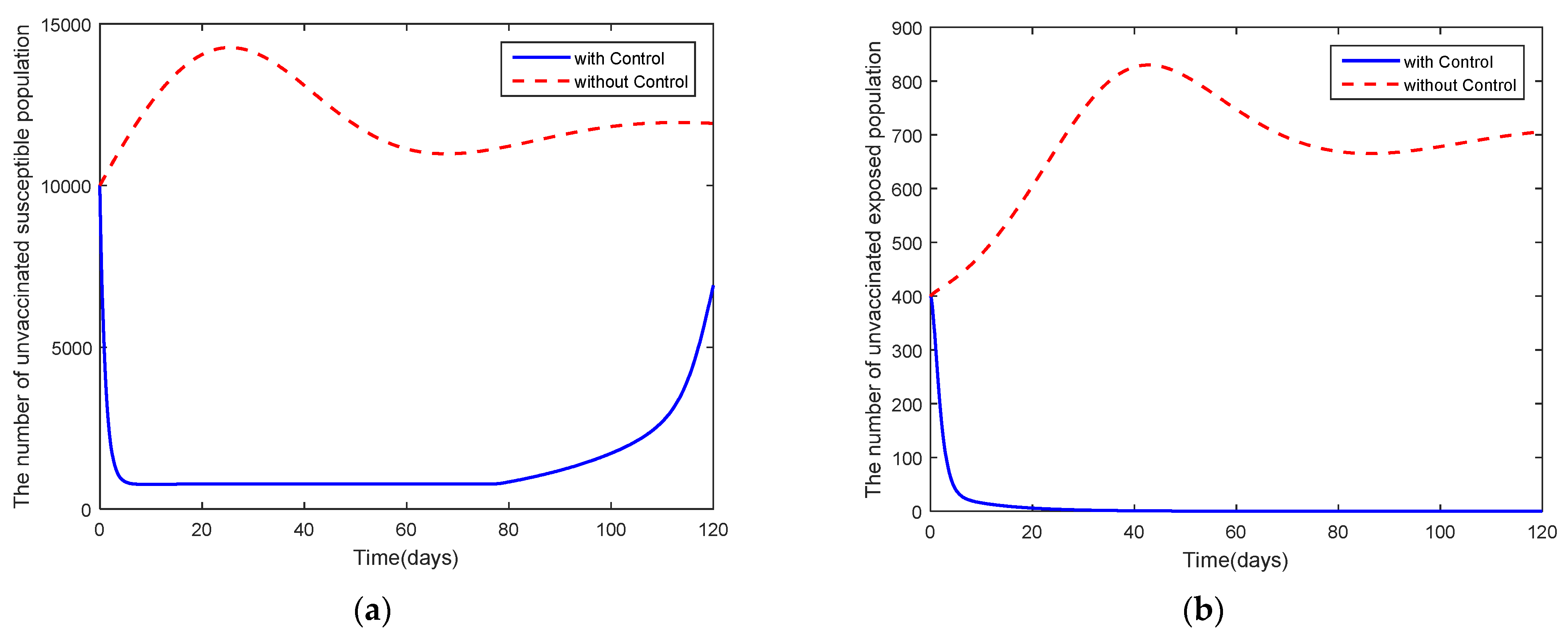
4. Optimal Control Problem

Having analyzed the mathematical model predicting the spread of the COVID-19 in Thailand, an optimal control strategy is now sought in order to help reduce the number of infected people and control and prevent the spread of the disease. In this article, a strategy for controlling COVID-19 in Thailand was proposed by considering the control functions, u 1 and u 2 , where u 1 is the rate of vaccination and u 2 is the susceptible group that is changed to the recovered group (due to immunity from the vaccination). According to the optimal control problem, the mathematical model for controlling COVID-19 can be created as follows:
d S n d t = ( 1 b ) σ η 1 S n μ S n u 1 ( t ) S n
d E n d t = η 1 S n ϕ E n ( 1 ϕ ) E n μ E n
d I a n d t = ϕ E n ( ω 1 + γ 2 + μ + d ) I a n
d I s n d t = ( 1 ϕ ) E n ( ω 2 + μ + d ) I s n
d S v d t = b σ η 2 S v μ S v u 2 ( t ) S v
d E v d t = η 2 S v ( 1 δ ) ϕ E v ( 1 δ ) ( 1 ϕ ) E v μ E v
d I a v d t = ( 1 δ ) ϕ E v ( ω 4 + γ 3 + μ + d ) I a v
d I a v d t = ( 1 δ ) ( 1 ϕ ) E v ( ω 3 + μ + d ) I s v
d H p d t = ω 1 I a n + ω 2 I s v + ω 3 I s v + ω 4 I a v ( γ 1 + μ + d ) H p
d R d t = γ 1 H p + γ 2 I a n + γ 3 I a v μ R + u 1 ( t ) S n + u 2 ( t ) S v
We now seek the optimal control strategy for the system of Equations (24)–(33) using Pontryagin’s maximum principle [40,41] to reduce the number of infected people, in other words, the optimal values u 1 and u 2 . In light of this, the optimal control problem is determined in terms of the following objective functions:
J ( u 1 ( t ) , u 2 ( t ) ) = 0 T ( A 1 I a n ( t ) + A 2 I s n ( t ) + A 3 I a v ( t ) + A 4 I s v ( t ) + 1 2 A 5 u 1 2 ( t ) + 1 2 A 6 u 2 2 ( t ) )
The objective function of the system of Equation (34) depends on hypotheses considering the number of I a n ( t ) ,   I s n ( t ) ,   I a v ( t ) , and I s v ( t ) . Please kindly note that A 1 ,   A 2 ,   A 3 ,   A 4 ,   A 5 , and A 6 are the weight constants. The most suitable problem solving guideline of this model is determined by using Lagrangian and Hamiltonian approaches to solve the optimal control problem as follows:
L ( I a n , I s n , I a v , I s v , u 1 , u 2 ) = A 1 I a n ( t ) + A 2 I s n ( t ) + A 3 I a v ( t ) + A 4 I s v ( t ) + 1 2 A 5 u 1 2 ( t ) + 1 2 A 6 u 2 2 ( t )
Theorem 3. 
With a suitable control  u * = ( u 1 * , u 2 * ) and a problem-solving guideline consistent with S n ,   E n ,   I a n ,   I s n ,   S v ,   E v ,   I a v ,   I s v ,   H p , and  R  for the initial problem (24)–(33)that the minimizes J ( u 1 , u 2 ) , there exists an adjoint variable   λ i ,   i = 1 , 2 , 3 , , 10 under the control that satisfies the following:
d λ i d t = H ψ
When ψ = ( S n , E n , I a n , I s n , S v , E v , I a v , I s v , H p , R ), together with the transversality conditions given as  λ i ( T ) = 0  for all  i = 1 , 2 , 3 , , 10 , and
u 1 * = { 0 i f     λ 1 S n λ 10 S n A 5 0 λ 1 S n λ 10 S n A 5     i f     λ 1 S n λ 10 S n A 5 < u 1 m a x u 1 m a x i f     λ 1 S n λ 10 S n A 5 u 1 m a x
u 2 * = { 0 i f     λ 5 S v λ 10 S v A 6 0 λ 5 S v λ 10 S v A 6 i f     λ 5 S v λ 10 S v A 6 < u 2 m a x u 2 m a x i f     λ 5 S v λ 10 S v A 6 u 2 m a x
Proof. 
The Hamiltonian function can be defined as
H = L ( I a n , I s n , I a v , I s v , u 1 , u 2 ) + λ 1 d S n d t + λ 2 d E n d t + λ 3 d I a n d t + λ 4 d I s n d t + λ 5 d S v d t + λ 6 d E v d t + λ 7 d I a v d t + λ 8 d I s v d t + λ 9 d H p d t + λ 10 d R d t
when
L ( I a n , I s n , I a v , I s v , u 1 , u 2 ) = A 1 I a n ( t ) + A 2 I s n ( t ) + A 3 I a v ( t ) + A 4 I s v ( t ) + 1 2 A 5 u 1 2 ( t ) + 1 2 A 6 u 2 2 ( t )
is the Lagrangian of the control problem, then we have
H = A 1 I a n ( t ) + A 2 I s n ( t ) + A 3 I a v ( t ) + A 4 I s v ( t ) + 1 2 A 5 u 1 2 ( t ) + 1 2 A 6 u 2 2 ( t ) + λ 1 [ ( 1 b ) σ η 1 S n μ S n u 1 ( t ) S n ] + λ 2 [ η 1 S n ϕ E n ( 1 ϕ ) E n μ E n ] + λ 3 [ ϕ E n ( ω 1 + γ 2 + μ + d ) I a n ] + λ 4 [ ( 1 ϕ ) E n ( ω 2 + μ + d ) I s n ] + λ 5 [ b σ η 2 S v μ S v u 2 ( t ) S v ] + λ 6 [ η 2 S v ( 1 δ ) ϕ E v ( 1 δ ) ( 1 ϕ ) E v μ E v ] + λ 7 [ ( 1 δ ) ϕ E v ( ω 4 + γ 3 + μ + d ) I a v ] + λ 8 [ ( 1 δ ) ( 1 ϕ ) E v ( ω 3 + μ + d ) I s v ] + λ 9 [ ω 1 I a n + ω 2 I s v + ω 3 I s v + ω 4 I a v ( γ 1 + μ + d ) H p ] + λ 10 [ γ 1 H p + γ 2 I a n + γ 3 I a v μ R + u 1 ( t ) S n + u 2 ( t ) S v ]
To obtain the optimal control, adjoint function becomes
d λ 1 d t = H S n = λ 1 ( t ) ( β a n I a n + β s n I s n + μ + u 1 * ( t ) ) λ 2 ( t ) ( β a n I a n + β s n I s n ) λ 10 ( t ) u 1 * ( t ) d λ 2 d t = H E n = λ 2 ( t ) ( 1 + μ ) λ 3 ( t ) ϕ λ 4 ( t ) ( 1 ϕ ) d λ 3 d t = H I a n = β a n S n ( λ 1 ( t ) λ 2 ( t ) ) + λ 3 ( t ) ( d + γ 2 + μ + ω 1 ) λ 9 ( t ) ω 1 λ 10 ( t ) γ 2 A 1 d λ 4 d t = H I s n = β s n S n ( λ 1 ( t ) λ 2 ( t ) ) + λ 4 ( t ) ( d + μ + ω 2 ) λ 9 ( t ) ω 2 A 2 d λ 5 d t = H S v = λ 5 ( t ) ( β a v I a v + β s v I s v + μ + u 2 * ( t ) ) λ 6 ( t ) ( β a v I a v + β s v I s v ) λ 10 ( t ) u 2 * ( t ) d λ 6 d t = H E v = λ 6 ( t ) ( μ + ( 1 δ ) ( 1 ϕ ) + ( 1 δ ) ϕ ) λ 7 ( t ) ( 1 δ ) ϕ λ 8 ( t ) ( 1 δ ) ( 1 ϕ ) d λ 7 d t = H I a v = β a v S v ( λ 5 ( t ) λ 6 ( t ) ) + λ 7 ( t ) ( d + γ 3 + μ + ω 4 ) λ 9 ( t ) ω 4 λ 10 ( t ) γ 3 A 3 d λ 8 d t = H I s v = β s v S v ( λ 5 ( t ) λ 6 ( t ) ) + λ 8 ( t ) ( d + μ + ω 3 ) λ 9 ( t ) ω 3 A 4 d λ 9 d t = H H p = λ 9 ( t ) ( d + μ + γ 1 ) λ 10 ( t ) γ 1 d λ 9 d t = H R = λ 10 ( t ) μ
The characterization of the suitable controls, u 1 *   and   u 2 * , depends on H u j = 0 for all j = 1 , 2 at u j = u j * at   j = 1 , 2 .
Therefore,
H u 1 = A 5 u 1 λ 1 S n + λ 10 S n u 1 * = λ 1 S n λ 10 S n A 5 H u 2 = A 6 u 2 λ 5 S v + λ 10 S v u 2 * = λ 5 S v λ 10 S v A 6
Thus, the optimal control function for COVID-19 can be defined as follows:
u 1 * = { 0 i f     λ 1 S n λ 10 S n A 5 0 λ 1 S n λ 10 S n A 5     i f     λ 1 S n λ 10 S n A 5 < u 1 m a x u 1 m a x i f     λ 1 S n λ 10 S n A 5 u 1 m a x
u 2 * = { 0 i f     λ 5 S v λ 10 S v A 6 0 λ 5 S v λ 10 S v A 6 i f     λ 5 S v λ 10 S v A 6 < u 2 m a x u 2 m a x i f     λ 5 S v λ 10 S v A 6 u 2 m a x
Figure 10 and Figure 11 show the numerical analysis of the optimal control policy. The equations were solved using the fourth order Runge–Kutta forward–backward sweep method [33]. For all simulation models, time T was determined to be 120 days. Controlled weight values were A 1 = 1000 ,   A 2 = 900 ,   A 3 = 700 ,   A 4 = 500 ,     A 5 = 300 ,   and A 6 = 100 . It can be clearly seen that the cases with control converged to an equilibrium point more quickly than the cases without the optimal control. As a consequence, it can be concluded that a good preventive policy through vaccination to develop immunity to the body is a suitable method to reduce the prevalence of the spread of the disease.

5. Discussion and Conclusions

This study shows the details of a mathematical model to control COVID-19, a pandemic currently infecting the world. It is based on the mathematical description of what is happening around the world. The current study is based on parameters which are appropriate in Thailand, one of the countries experiencing the infection. The mathematical model is created by considering two groups of people: the unvaccinated people and the vaccinated people. Standard dynamic modeling is used to study, analyze, and find the equilibrium points and establish stability. From this study, two equilibrium points were obtained, namely the disease-free equilibrium point ( G 0 * ) and the endemic equilibrium point ( G 1 * ) , according to parameter conditions. The Lyapunov function was used to determine the stability of each equilibrium point. From the simulation model, the basic reproduction number ( R 0 ) was obtained by considering the basic reproduction number of the disease-free steady states and the endemic steady states. It can be seen that the disease-free steady states are stable when ( R 0 < 1 ) and the endemic steady states are stable when ( R 0 > 1 ) . According to t h e   sensitivity analysis of the parameters, the efficacy of vaccination ( b ) and the infection rates ( β a n ,     β s n ,   β a v ,   and   β s v ) are the most sensitive parameters that contribute to an increase in the spread of COVID-19. It is noticeable that the infection rate is highly important. Therefore, to design a usable optimal control strategy for containing the spread of the Omicron variant in Thailand, a curve fitting algorithm was performed on the real-world Omicron data to analyze and seek the most suitable value of the infection rate to ensure it is similar to the current situation. The results in Figure 2 confirmed that this is so.
To examine and confirm the analysis results for the effects of the spread, parameter values were chosen to be the values given in Table 2, incorporating the fitted parameters. According to Figure 5, considering of the efficacy of the vaccines, it was found that if the efficacy of the vaccines increases, spread control is achieved more quickly. Considering the infection rate showed that when the rate of spread increased, the basic reproduction number increased, since the basic reproduction number is the average number of secondary infections which can be caused by a patient in a completely susceptible population throughout his infectious period. If the infection rate is high, the epidemic shall spread at a slower rate when the infection rate is low. Therefore, if the basic reproduction number is high, the epidemic would spread at a fast rate and converge to an equilibrium point more quickly when the basic reproduction is low. From what was mentioned above, it can be seen that Figure 6, Figure 7, Figure 8 and Figure 9 follow the above-mentioned conditions. Nonetheless, there are a lot of factors affecting the spread. The spread can be minimized by planning and formulating policies. In this regard, the optimal control strategy is used by considering the rate of vaccination and immunity achieved from vaccination to reduce the spread of COVID-19. It can be concluded that the spread of COVID-19 can be controlled and minimized by vaccination and self-care practices following preventive measures, as seen in Figure 10 and Figure 11. Note that the main limitation of our model is that we did not use the multiple-patch model, where the Omicron outbreak in the rural regions is different from the one in the city because of the population density and socioeconomics. Nevertheless, the model used in this paper is simple enough to capture the main dynamics of the system and allows for the conjuration of suitable optimal control to combat the spread.
In conclusion, the use of the control strategy for disease prevention is a guideline to help prevent and control the spread of the disease. There are many strategies for disease control, such as social distancing, wearing masks, or following preventive measures introduced by the government. Future research should determine other strategies to help control and prevent COVID-19, accordingly.

Author Contributions

Conceptualization, J.L., P.P. and N.W.; methodology, J.L.; software, N.W.; validation, J.L., P.P., I.-M.T. and N.W.; writing—original draft preparation, J.L.; writing—review and editing, J.L., P.P., I.-M.T. and N.W.; supervision, P.P., I.-M.T. and N.W.; project administration, P.P.; funding acquisition, P.P. All authors have read and agreed to the published version of the manuscript.

Funding

This work is supported by the School of Science, King Mongkut’s Institute of Technology Ladkrabang, Grant Number (2564-02-05-008).

Data Availability Statement

Data are available from the corresponding author upon reasonable request.

Acknowledgments

Jiraporn Lamwong is the recipient of the Graduate Study Fellowship of the School of Science, King Mongkut’s Institute of Technology Ladkrabang, Thailand. This research was funded by the RA-TA graduate scholarship from the School of Science, King Mongkut’s Institute of Technology Ladkrabang, grant number RA/TA-2565-D-001.

Conflicts of Interest

The authors declare no conflict of interest.

References

  1. Chaharborj, S.S.; Hassanzadeh, J.; Phang, P.C. Controlling of pandemic COVID-19 using optimal control theory. Results Phys. 2021, 26, 104311. [Google Scholar] [CrossRef]
  2. Jankhonkhan, J.; Sawangtong, W. Model Predictive Control of COVID-19 pandemic Concerning Social Isolation and Vaccination Policies in Thailand. Axioms 2021, 10, 274. [Google Scholar] [CrossRef]
  3. Lina, Q.; Zhaob, S.; Gaod, D.; Loue, Y.; Yangf, S.; Musae, S.S.; Wangb, M.H.; Caig, Y.; Wangg, W.; Yangh, L.; et al. A conceptual model for the coronavirus disease 2019 (COVID-19) outbreak in Wuhan, China with individual reaction and governmental action. Int. J. Infect. Dis. 2020, 93, 211–216. [Google Scholar] [CrossRef]
  4. Feng, L.X.; Jing, S.L.; Hu, S.K.; Wang, D.F.; Huo, H.F. Modelling the effects of media coverage and quarantine on the COVID-19 infections in the UK. Math. Biosci. Eng. 2020, 17, 3618–3636. [Google Scholar] [CrossRef]
  5. Prathumwan, D.; Trachoo, K.; Chaiya, I. Mathematical Modeling for Prediction Dynamics of the Coronavirus Disease 2019 (COVID-19) Pandemic, Quarantine Control Measures. Symmetry 2020, 12, 1404. [Google Scholar] [CrossRef]
  6. Win, Z.T.; Eissa, M.A.; Tian, B. Stochastic Epidemic Model for COVID-19 Transmission under Intervention Strategies in China. Mathematics 2022, 10, 3119. [Google Scholar] [CrossRef]
  7. Yang, C.; Wang, J. Modeling the transmission of COVID-19 in the US-A case study. Infect. Dis. Model. 2021, 6, 195–211. [Google Scholar] [CrossRef]
  8. Zhanga, Z.; Jain, S. Mathematical model of Ebola and Covid-19 with fractional differential operators: Non-Markovian process and class for virus pathogen in the environment. Chaos Solit. Fract. 2020, 140, 110175. [Google Scholar] [CrossRef]
  9. Diagne, M.L.; Rwezaura, H.; Tchoumi, S.Y.; Tchuenche, J.M. A Mathematical Model of COVID-19 with Vaccination and Treatment. Comput. Math. Methods Med. 2021, 2021, 1250129. [Google Scholar] [CrossRef]
  10. Iboi, E.A.; Sharomi, O.; Ngonghala, C.N.; Gumel, A.B. Mathematical modeling and analysis of COVID-19 pandemic in Nigeria. Math. Biosci. Eng. 2020, 17, 7192–7220. [Google Scholar] [CrossRef]
  11. Ndaïrou, F.; Area, L.; Nietoc, J.J.; Torres, D.F.M. Mathematical modeling of COVID-19 transmission dynamics with a case study of Wuhan. Chaos Solit. Fract. 2020, 135, 109846. [Google Scholar] [CrossRef] [PubMed]
  12. Faruk, O.; Kar, S. A Data Driven Analysis and Forecast of COVID-19 Dynamics during the Third Wave Using SIRD Model in Bangladesh. COVID 2021, 1, 43. [Google Scholar] [CrossRef]
  13. Wang, L.; Dai, Y.; Wang, R.; Sun, Y.; Zhang, C.; Yang, Z.; Sun, Y. SEIARN: Intelligent Early Warning Model of Epidemic Spread Based on LSTM Trajectory Prediction. Mathematics 2022, 10, 3046. [Google Scholar] [CrossRef]
  14. World Health Organization. COVID-19—WHO Thailand Situation Reports. Available online: https://www.who.int/thailand/emergencies/novel-coronavirus-2019/situation-reports (accessed on 29 June 2022).
  15. Kermack, W.O.; McKndrick, A.G.; Walker, G.T. A contribution to the mathematical theory of epidemics. R. Soc. Lond. Ser. A Contain. Pap. Math. Phys. Charact. 1927, 115, 700–721. [Google Scholar]
  16. Lamwong, J.; Pongsumpun, P.; Tang, I.M.; Wongvanich, N. The Lyapunov Analyses of MERS-Cov Transmission in Thailand. Curr. Appl. Sci. Technol. 2019, 19, 112–123. [Google Scholar]
  17. Etbaigha, F.; Willms, A.R.; Poljak, Z. An SEIR model of influenza A virus infection and reinfection within a farrow-to-finish swine farm. PLoS ONE 2018, 13, e0202493. [Google Scholar] [CrossRef] [Green Version]
  18. Islam, R.; Biswas, M.H.A.; Jamali, A.R.M. Mathematical analysis of Epidemiological Model of Influenza A (H1N1) Virus Transmission Dynamics in Bangladesh Perspective. GANIT J. Bangladesh. Math. Soc. 2017, 37, 39–50. [Google Scholar] [CrossRef]
  19. Rezapour, S.; Mohammadi, H. A study on the AH1N1/09 influenza transmission model with the fractional Caputo–Fabrizio derivative. Adv. Diff. Equ. 2020, 2020, 488. [Google Scholar] [CrossRef]
  20. Chanprasopchai, P.; Pongsumpun, P.; Tang, I.M. Effect of Rainfall for the Dynamical Transmission Model of the Dengue Disease in Thailand. Comput. Math. Methods Med. 2017, 2017, 17. [Google Scholar] [CrossRef] [Green Version]
  21. Bhuju, G.; Phaijoo, G.R.; Gurung, D.B. Fuzzy Approach Analyzing SEIR-SEI Dengue Dynamics. Biomed. Res. Int. 2020, 2020, 11. [Google Scholar] [CrossRef]
  22. Gardner, L.M.; Rey, D.; Heywood, A.E.; Toms, R.; Wood, J.; Travis Waller, S.; Raina MacIntyre, C. A scenario-based evaluation of the Middle East respiratory syndrome coronavirus and the Hajj. Risk. Anal. 2014, 34, 1391–1400. [Google Scholar] [CrossRef] [PubMed] [Green Version]
  23. Sen, D.; Sen, D. Use of a Modified SIRD Model to Analyze COVID-19 Data. Ind. Eng. Chem. Res. 2021, 60, 4251–4260. [Google Scholar] [CrossRef]
  24. Kumar, H.; Arora, P.K.; Pant, M.; Kumar, A.; Shahroz, A.K. A simple mathematical model to predict and validate the spread of Covid-19 in India. Mater. Today Proc. 2021, 47, 3859–3864. [Google Scholar] [CrossRef] [PubMed]
  25. Hezam, I.M.; Foul, A.; Alrasheedi, A. A dynamic optimal control model for COVID-19 and cholera co-infection in Yemen. Adv. Differ. Equ. 2021, 2021, 108. [Google Scholar] [CrossRef]
  26. Riyapan, P.; Shuaib, S.E.; Intarasit, A. A Mathematical Model of COVID-19 Pandemic: A Case Study of Bangkok, Thailand COVID-19. Comput. Math. Methods Med. 2021, 2021, 6664483. [Google Scholar] [CrossRef]
  27. Rajput, A.; Sajid, M.; Tanvi; Shekhar, C.; Aggarwal, R. Optimal control strategies on COVID-19 infection to bolster the efcacy of vaccination in India. Sci. Rep. 2021, 11, 20124. [Google Scholar] [CrossRef]
  28. Dipo Aldila, D.; Shahzad, M.; Khoshnaw, A.H.A.; Ali, M.; Sultan, F.; Islamilova, A.; Anwar, Y.R.; Samiadji, B.M. Optimal control problem arising from COVID-19 transmission model with rapid-test. Results Phys. 2020, 37, 105501. [Google Scholar] [CrossRef]
  29. Tchoumi, S.Y.; Diagne, M.L.; Rwezaurac, H.; Tchuenche, J.M. Malaria and COVID-19 co-dynamics: A mathematical model and optimal control. Appl. Math. Model. 2021, 99, 294–327. [Google Scholar] [CrossRef]
  30. Driessche, P.V.; Watmough, J. Reproduction numbers and sub-threshold endemic equilibria for compartmental models of disease transmission. Math. Biosci. 2020, 180, 29–48. [Google Scholar] [CrossRef]
  31. Abioye, A.I.; Peter, O.J.; Ogunseye, H.A.; Oguntolu, F.A.; Oshinubi, K.; Ibrahim, A.A.; Khan, I. Mathematical model of COVID-19 in Nigeria with optimal control. Results Phys. 2020, 28, 104598. [Google Scholar] [CrossRef]
  32. La Salle, J.P. The Stability of Dynamical Systems; Society for Industrial and Applied Mathematics: Philadelphia, PA, USA, 1976. [Google Scholar]
  33. Adepoju, O.A.; Samson Olaniyi, S. Stability and optimal control of a disease model with vertical transmission and saturated incidence. Sci. Afri. 2021, 12, e00800. [Google Scholar] [CrossRef]
  34. Gatyeni, S.P.; Chirove, F.; Nyabadza, F. Modelling the Potential Impact of Stigma on the Transmission Dynamics of COVID-19 in South Africa. Mathematics 2022, 10, 3253. [Google Scholar] [CrossRef]
  35. Lahodny, G. Curve Fitting and Parameter Estimation; Springer: Berlin/Heidelberg, Germany, 2015; pp. 1–18. [Google Scholar]
  36. Arruda, E.F.; Das, S.S.; Dias, C.M.; Pastore, D.H. Modelling and optimal control of multi strain epidemics, with application to COVID-19. PLoS ONE 2021, 16, e0257512. [Google Scholar] [CrossRef] [PubMed]
  37. Lamwong, J.; Tang, I.; Pongsumpun, P. Mers model of Thai and South Korean population. Curr. Appl. Sci. Technol. 2018, 18, 45–57. [Google Scholar]
  38. Husniah, H.; Ruhanda, R.; Supriatna, A.K.; Biswas, M.H.A. SEIR Mathematical Model of Convalescent Plasma Transfusion to Reduce COVID-19 Disease Transmission. Mathematics 2021, 9, 2857. [Google Scholar] [CrossRef]
  39. Chitnis, N.; Hyman, J.M.; Cushing, J.M. Determining important parameters in the spread of malaria through the sensitivity analysis of a mathematical model. Bull. Math. Biol. 2008, 70, 1272–1296. [Google Scholar] [CrossRef]
  40. Lenhart, S.; Workman, J.T. Optimal Control Applied to Biological Models; Chapman & Hall/CRC: London, UK, 2007. [Google Scholar]
  41. Pontryagin, L.S.; Boltyanskii, V.G.; Gamkrelidze, R.V.; Mishchenko, E.F. The Mathematical Theory of Optimal Processes; Wiley: New York, NY, USA, 1962. [Google Scholar]
Figure 1. Diagram showing the relationship of the COVID-19 mathematical model and vaccination.
Mathematics 10 03899 g001
Figure 2. Data fitting of the model (3)–(12) to the actual data: (a) susceptible with vaccinated fitting; (b) susceptible with unvaccinated fitting.
Mathematics 10 03899 g002
Figure 3. Graphs of the system of Equations (3)–(12) at the disease-free equilibrium point of S n ,   E n ,   I a n ,   I s n ,   S v ,   E v ,   I a v ,   I s v ,   H p , and   R when R 0 < 1 : (a) the number in the unvaccinated, susceptible population; (b) the number in the unvaccinated, exposed population; (c) the number in the unvaccinated, asymptomatic, infected population; (d) the number in the unvaccinated, symptomatic, infected population; (e) the number in the vaccinated, susceptible population; (f) the number in the vaccinated, exposed population; (g) the number in the vaccinated, asymptomatic, infected population; (h) the number in the vaccinated, symptomatic, infected population; (i) the number in the hospitalized population; and (j) the number in the recovered population.
Mathematics 10 03899 g003aMathematics 10 03899 g003bMathematics 10 03899 g003c
Figure 4. Graphs of the system Equations (3)–(12) at the endemic equilibrium point of S n ,   E n ,   I a n ,   I s n ,   S v ,   E v ,   I a v ,   I s v ,   H p , and   R when R 0 > 1 : (a) the number in the unvaccinated, susceptible population; (b) the number in the unvaccinated, exposed population; (c) the number in the unvaccinated, asymptomatic, infected population; (d) the number in the unvaccinated, symptomatic, infected population; (e) the number in the vaccinated susceptible population; (f) the number in the vaccinated, exposed population; (g) the number in the vaccinated, asymptomatic, infected population; (h) the number in the vaccinated, symptomatic, infected population; (i) the number in the hospitalized population; and (j) the number in the recovered population.
Mathematics 10 03899 g004aMathematics 10 03899 g004b
Figure 5. Graphs of the system of Equations (3)–(12) showing the comparison results of efficacy of vaccination ( b ) when R 0 > 1 : (a) the number in the unvaccinated, susceptible population; (b) the number in the unvaccinated, exposed population; (c) the number in the unvaccinated, asymptomatic, infected population; and (d) the number in the unvaccinated, symptomatic, infected population.
Mathematics 10 03899 g005
Figure 6. Graphs of the system of Equations (3)–(12) showing the comparison results of the infection rate of the asymptomatic, unvaccinated, infected population ( β a n ) when R 0 > 1 : (a) the number in the unvaccinated, susceptible population; (b) the number in the unvaccinated, exposed population; (c) the number in the unvaccinated, asymptomatic, infected population; and (d) the number in the unvaccinated, symptomatic, infected population.
Mathematics 10 03899 g006
Figure 7. Graphs of the system of Equations (3)–(12) showing the comparison results of the infection rate of the symptomatic, unvaccinated, infected population ( β s n ) when R 0 > 1 : (a) the number in the unvaccinated, susceptible population; (b) the number in the unvaccinated, exposed population; (c) the number in the unvaccinated, asymptomatic, infected population; and (d) the number in the unvaccinated, symptomatic, infected population.
Mathematics 10 03899 g007aMathematics 10 03899 g007b
Figure 8. Graphs of the system of Equations (3)–(12) showing the comparison results of the infection rate of the asymptomatic, vaccinated, infected population ( β a v ) when R 0 > 1 : (a) the number in the vaccinated, susceptible population; (b) the number in the vaccinated, exposed population; (c) the number in the vaccinated, asymptomatic, infected population; and (d) the number in the vaccinated, symptomatic, infected population.
Mathematics 10 03899 g008
Figure 9. Graphs of the system of Equations (3)–(12) showing the comparison results of the infection rate of the symptomatic, vaccinated, infected population ( β s v ) when R 0 > 1 : (a) the number in the vaccinated, susceptible population; (b) the number in the vaccinated, exposed population; (c) the number in the vaccinated, asymptomatic, infected population; and (d) the number in the vaccinated, symptomatic, infected population.
Mathematics 10 03899 g009
Figure 10. Comparison between the cases with control and the cases without control for the disease-free: (a) the number in the unvaccinated, susceptible population; (b) the number in the unvaccinated, exposed population; (c) the number in the unvaccinated, asymptomatic, infected population; (d) the number in the unvaccinated, symptomatic, infected population; (e) the number in the vaccinated, susceptible population; (f) the number in the vaccinated, exposed population; (g) the number in the vaccinated, asymptomatic, infected population; (h) the number in the vaccinated, symptomatic, infected population; (i) the number in the hospitalized population; (j) the number in the recovered population; and (k) control efforts u 1 ( t ) and u 2 ( t ) .
Mathematics 10 03899 g010aMathematics 10 03899 g010bMathematics 10 03899 g010c
Figure 11. Comparison between the cases with control and the cases without control for the endemic: (a) the number in the unvaccinated, susceptible population; (b) the number in the unvaccinated, exposed population; (c) the number in the unvaccinated, asymptomatic, infected population; (d) the number in the unvaccinated, symptomatic, infected population; (e) the number in the vaccinated, susceptible population; (f) the number in the vaccinated, exposed population; (g) the number in the vaccinated, asymptomatic, infected population; (h) the number in the vaccinated, symptomatic, infected population; (i) the number in the hospitalized population; (j) the number in the recovered population; and (k) control efforts u 1 ( t ) and u 2 ( t ) .
Mathematics 10 03899 g011aMathematics 10 03899 g011bMathematics 10 03899 g011c
Table 1. Definitions of variables and parameters.
Variables and ParametersDescription
S n The number in the unvaccinated, susceptible population.
E n The number in the unvaccinated, exposed population.
I a n The number in the unvaccinated, asymptomatic, infected population.
I s n The number in the unvaccinated, symptomatic, infected population.
S v The number in the vaccinated, susceptible population.
E v The number in the vaccinated, exposed population.
I a v The number in the vaccinated, asymptomatic, infected population.
I s v The number in the vaccinated, symptomatic, infected population.
H p The number in the hospitalized population.
R The number in the recovered population.
b Efficacy of vaccination.
σ Initial number in the population.
β a n Infection rate of the unvaccinated, asymptomatic, infected population.
β s n Infection rate of the unvaccinated, symptomatic, infected population.
β a v Infection rate of the vaccinated, asymptomatic, infected population.
β s v Infection rate of the vaccinated, symptomatic, infected population.
ϕ Incubation period of the disease.
δ Efficacy of the vaccination against COVID-19.
ω 1 Hospitalization rate of the unvaccinated, asymptomatic, infected population.
ω 2 Hospitalization rate of the unvaccinated, symptomatic, infected population.
ω 3 Hospitalization rate of the vaccinated, asymptomatic, infected population.
ω 4 Hospitalization rate of the vaccinated, symptomatic, infected population.
γ 1 Recovery rate after hospitalization.
γ 2 Recovery rate of the unvaccinated, asymptomatic, infected population.
γ 3 Recovery rate of the vaccinated, asymptomatic, infected population.
μ Death rate from natural causes.
d Death rate from COVID-19.
N h Total number in the human population.
Table 2. The parameters used in the numerical simulation.
ParametersThe Disease-FreeThe EndemicReference
b 0.50.5Estimated
σ 11400Estimated
β a n 0.000010.00001Data fitted
β s n 0.0000090.000009Data fitted
β a v 0.0000080.000008Data fitted
β s v 0.000010.00001Data fitted
ϕ 1/71/7[7,36]
δ 0.80.8Assumed
ω 1 0.10.1[5,7]
ω 2 0.10.1[5,7]
ω 3 0.10.1[5,7]
ω 4 0.10.1[5,7]
γ 1 1/71/7[7]
γ 2 1/141/14[10]
γ 3 1/141/14[7]
μ 0.00003650.0000365[37,38]
d 0.002860.00286[31]
Table 3. Sensitivity values of the basic reproduction numbers.
ParametersSensitivity Indices
b +1.0000
σ +1.0000
β a n +0.1209
β s n +0.8791
β a v +0.0730
β s v +0.9270
δ +0.0007
ϕ −0.0026
ω 1 −0.0872
ω 2 −0.8544
ω 3 −0.9009
ω 4 −0.0419
γ 1 −0.0311
γ 2 −0.0299
γ 3 −1.0004
μ −0.0269
Publisher’s Note: MDPI stays neutral with regard to jurisdictional claims in published maps and institutional affiliations.

