Article

Cattle Number Estimation on Smart Pasture Based on Multi-Scale Information Fusion

1
College of Computer Science and Engineering, Chongqing University of Technology, Chongqing 400054, China
2
School of Computing, Teesside University, Middlesbrough TS1 3BX, UK
*
Author to whom correspondence should be addressed.
Mathematics 2022, 10(20), 3856; https://doi.org/10.3390/math10203856
Submission received: 7 August 2022 / Revised: 13 October 2022 / Accepted: 14 October 2022 / Published: 18 October 2022
(This article belongs to the Special Issue Advances in Computer Vision and Machine Learning)

Abstract

:
In order to solve the problem of intelligent management of cattle numbers in the pasture, a dataset of cattle density estimation was established, and a multi-scale residual cattle density estimation network was proposed to solve the problems of uneven distribution of cattle and large scale variations caused by perspective changes in the same image. Multi-scale features are extracted by multiple parallel dilated convolutions with different dilation rates. Meanwhile, aiming at the “grid effect” caused by the use of dilated convolution, the residual structure is combined with a small dilation rate convolution to eliminate the influence of the “grid effect”. Experiments were carried out on the cattle dataset and dense population dataset, respectively. The experimental results show that the proposed multi-scale residual cattle density estimation network achieves the lowest mean absolute error (MAE) and means square error (RMSE) on the cattle dataset compared with other density estimation methods. In ShanghaiTech, a dense population dataset, the density estimation results of the multi-scale residual network are also optimal or suboptimal in MAE and RMSE.

1. Introduction

In farm management, cattle numbers estimation is one of the most critical tasks in asset valuation and pasture management. Precise cattle counts improve the efficiency of farming during assessing assets. It also helps both companies and individuals to reduce unnecessary losses as it detects theft in time [1]. In practice, cattle counting in farms can be challenging because of different factors, such as cattle’s overlapping [2], scene transformation [3], and environmental illumination changing [4]. The traditional method, e.g., counting by human, is often very time consuming, labour intensive and error-prone [5].
Vision-based target counting has gained much attention in recent years. Many scenarios have utilised digital image processing methods for target counting, such as dense crowd counting [6,7,8,9,10,11], crop target counting [12,13], cell counting [14], small target counting [15]. However, visual-based counting technologies have been poorly studied in animal husbandry and are mostly hardware-based methods.
Deep learning has made good progress in recent years for the crowd density estimation problem [16]. Crowd density estimation aims to obtain a predicted density graph by learning a mapping between the local features of an image and its corresponding density graph. The density graph represents the distribution of the crowd and the number of people at each pixel point. The estimated crowd size is finally obtained by integral and summing the density graphs. In farm management, crowd density estimation based on convolutional neural networks has achieved good performance in chicken [17] and pineapple flower counting [18], but the application on cattle counting is still limited.
Here we first clarify the problem as three main tasks: (1) uneven distribution of cattle, (2) scale variations caused by perspective, (3) grid effect. Uneven distribution is one of the most significant problems in crowd density estimation. In our collected pasture dataset, cattle distribution varies in different scenes. Scale variations occur on both fish-eye cameras and ordinary cameras; it requires a well-trained model to describe images that are more flexible and robust. Grid effect is inevitable when our model superposes multiple dilated convolutions to analyse the dataset. A high dilation rate can lead to ignorance of critical features, which limits the model performance.
The cattle in image often have very different sizes, ranging from several pixels to tens of pixels. This requires the network to be able to capture a large rang of scales. This paper proposed a multi-scale residual cattle density estimate network called MSRNet, which is built upon the blocks consisting of densely connected dilated convolutional layers. Thus, it can output features having different receptive fields and capture cattle different scales. The MSR block obtains multi-scale receptive fields by using multi-column dilated convolution, and at the same time reduces the grid effect problem caused by continuous dilated convolution, as shown in Figure 1. So using multiple parallels dilated convolution to extract features is effective for the first two tasks. Using residual structure combined with small dilation rate convolution can help mitigate the grid effect. We summarise our contributions as follows:
  • Collect a novel herd image dataset in a variety of scenes and conditions.
  • Train a multi-scale residual cattle density estimate network (MSRNet) for cattle number estimation on both public dataset and collected dataset, and demonstrate the interpretability.
  • Identify three challenges on this dataset and utilize MSRNet to handle them. Conduct extensive experimentation to demonstrate the performance.
In addition, in contrast to traditional crowd density estimation, crowd datasets are usually labeled with heads of people, while cattle dataset is labeled with body of cattle. Since there is no public cattle dataset, we created a cattle density dataset and verify the effectiveness of our method on this dataset.
The remainder of the paper is structured as follows. Section 2 reviews existing methods to estimate cattle numbers and relative deep learning methods. In Section 3, we present details for the proposed methodology, including dataset collection and multi-scale residual cattle density estimation methods. After that, we demonstrate details about our dataset and the experimental results in Section 4 and discuss possible future works. Finally, we draw important conclusions in Section 5.

2. Related Work

The mainstream counting methods nowadays, both nationally and internationally, are hardware-based. The informatization achievement in the livestock breeding process is mainly based on electronic ear tags used as the core information carrier. However, there are still lots of promotion problems, such as high maintenance costs and complicated operations, in the livestock breeding industry. As a result, the large-scale application is limited at present [5]. Moreover, wearing ear tags can also bring some harm to the livestock itself, such as wound infection and calf panic [19]. There are three main types of vision-based counting methods: detection-based methods, regression-based methods and density-estimation-based methods.

2.1. Detection-Based Methods

Some researchers have used target detection methods to count livestock. Xu and her colleagues [20] used images captured by a drone to detect targets and segment livestock through Mask-RCNN to achieve live cattle counting in pasture and farm scenarios. Li et al. [21] used the YOLOv3 target detection algorithm combined with the Deep SORT target tracking algorithm to achieve automatic counting of sheep based on the bilinear counting method. All these methods mentioned above are only applicable to scenes where the targets are relatively sparse.

2.2. Regression-Based Methods

However, in the actual scenario of pastureland, there are usually different perspective variations in the images captured by the camera, resulting in large scale variations of the cattle. Most of the time, the cattle are clustered together and heavily obscured when the counting error of the target detection method is large. Researchers try to deploy regression-based methods to learn the relations among extracted features from cropped image patches, and then calculate the number of particular objects. Idrees et al. [6] proposed a model to extract features by employing Fourier analysis and SIFT (Scale invariant feature transform) [22] interest-point based counting.

2.3. Density Estimation-Based Methods

When executing the regression-based solution, one critical feature, called saliency, is overlooked which causes inaccurate results in local regions. Tian et al. [23] estimated the number of pigs in a pen by predicting the density of pigs in the image, and this method was more accurate for dense pig predictions compared to target detection but was inaccurate for numbers over 10. Density estimation can be divided into multi-column networks and single-column networks according to network structure. Multi-column networks refer to models containing multiple convolution columns, with different columns corresponding to different sizes of targets. Zhang et al first proposed the multi-column convolutional structure network MCNN [7], which consists of three columns of convolutions, each with a different size of the perceptual field to extract features at different scales. However, subsequent experiments found that the features extracted by this method were very redundant, and the structure limited the performance. Li et al. [8] proposed CSRNet to increase the perceptual field by stacking the dilated convolutions without reducing the image resolution, which improved the prediction accuracy. Wan et al. [24] used an adjustment network KDMG to dynamically adjust the supervised information for the problem of inaccurate label information generation and achieved good results in crowd density estimation. Although crowd density estimation networks are now better developed, very few studies have attempted deep learning-based density estimation algorithms in livestock industries such as cattle herding.

2.4. Common Public Datasets

Crowd counting and density estimation models based on deep learning highly rely on the dataset. There are four most commonly used datasets: UCSD [25], UCF_CC_50 [6], WorldExpo [26], ShanghaiTech_A and ShanghaiTech_B [7]. They contain 2000, 50, 3980, 482 and 716 image data, respectively. ShanghaiTech_A and ShanghaiTech_B are the largest datasets so far in terms of the annotated heads for crowd counting. However, all these datasets demonstrate human society scenarios, such as pedestrians on the sidewalk, public rallies, and sports events. Shao and his colleagues [27] collected a cattle counting dataset in 2018. It contains 670 images taken by an unmanned aerial vehicle (UAV), and the total target number is 218. But the data quantity and UAV scenario still limit the model application as most pastures still use fixed-position cameras instead of UAVs.
This paper proposed a multi-scale residual cattle density estimate network to estimate the number of cattle in a pasture. To address the problems of uneven distribution of cattle density and large scale variation of cattle in the same image, we proposed a multi-scale residual feature perception module that obtains a multi-scale perceptual field. It overcomes the grid problem caused by continuous dilated convolution by using multi-column dilated convolution. As there is no publicly available cattle herd dataset, we also collected and introduced a cattle herd density dataset in this paper, and we conducted extensive experimentation to demonstrate our model performance on this dataset. The cattle dataset is available at https://github.com/menjure/Cattle-dataset, accessed on 5 August 2022.

3. Methodology

The fundamental idea of our approach is to deploy an end-to-end multi-scale residual cattle density estimate network with denser scale diversity to cope with the large scale variations and density level differences in both congested and sparse scenes. In this section, we first introduce the generation of density maps, then we describe the architecture of MSRNet, next we explain the loss function, and finally we present the collected dataset.

3.1. Formalization

The goal of our MSRNet model is to generate a density map according to the given input pastures image. The task can be formalized as a mapping: F : X D , where X is the input image, D represents the output density map, respectively.
Different from the traditional regression methods that only return a crowd number, the density map provides more information. The image data are labelled with cattle number and position, and the density map will match the target distribution of the ground truth.
The performance of the networks depends heavily on the quality of the supervised data. A high-quality density graph can help improve the performance of the density estimation model in training. Generating a density graph consists of two steps: (1) cattle images annotation, (2) converting the cattle image labels to a cattle density graph. Specifically, let a cow at position x i be represented as δ ( x x i ) . In this way, an annotated image marked as N cows can be represented as a function below:
H x = i = 1 N δ ( x x i ) .
In a real image, each cow is of a certain size range and corresponds to a small image area. Setting the value of a pixel to 1 in the annotation file to represent this cow is unreasonable. The Gaussian kernel function is a distributed bell-shaped line, and the closer the coordinates are to the centre, the larger the value, and vice versa. So we use a Gaussian kernel function to replace the pixel value of this central point with a weighted average of the pixel values of the points around it. In this way, the weights of the pixel points within the blur radius add up to 1. This method does not affect the total number of cattle in the resulting density graph but also provides more realistic space location features of each cattle in the picture. For each image i, the annotated image function is convolved with a Gaussian kernel to obtain the density below:
D i g t = H i ( x ) · G σ ( x ) ,
where D i g t is the density supervisory information and σ is the Gaussian covariance.
The single-camera cattle density estimation is challenging because of the occlusion, uneven distribution, scale variations, and grid effect. Here we introduced the collected dataset below and described the multi-scale residual cattle density estimate network. Specifically, we first presented the overall framework of the network. Then, there is a detailed description of the multi-scale residual feature-aware module. In the end, we also discussed the loss function used in this paper.

3.2. Multi-Scale Residual Cattle Density Estimation Methods

3.2.1. MSRNet Structure

In order to efficiently deal with the uneven distribution of cattle density and large scale variation, a multi-scale residual network (MSRNet) is proposed. The proposed MSRNet structure is illustrated in Figure 2, which consists of a front-end feature extraction network and three back-end multi-scale feature sensing modules. In particular, the first ten convolutional layers and three pooling layers of the conventional VGG-16 [28] network are performed here, acting as the front-end feature extraction. The back-end consists of three multi-scale residual feature-aware modules. First, MSRNet apply their multi-scale perceptual fields to extract deeper semantic information, and then a density regression head is applied to obtain the final predicted density graph. The final number of predictions is obtained by integrating the predicted density graph.

3.2.2. Multi-Scale Residual Feature Sensing Module (MSR)

The MSR module is proposed to extract more and deeper semantic information. Each MSR module contains three dilated convolution layers and two conventional convolution layers, as shown in Figure 2. Compared with the conventional convolution operation, the dilated convolution, proposed by Yu et al. [29] for solving the image segmentation problem, introduces a “dilation rate” hyperparameter to increase the perceptual field without reducing the image resolution.
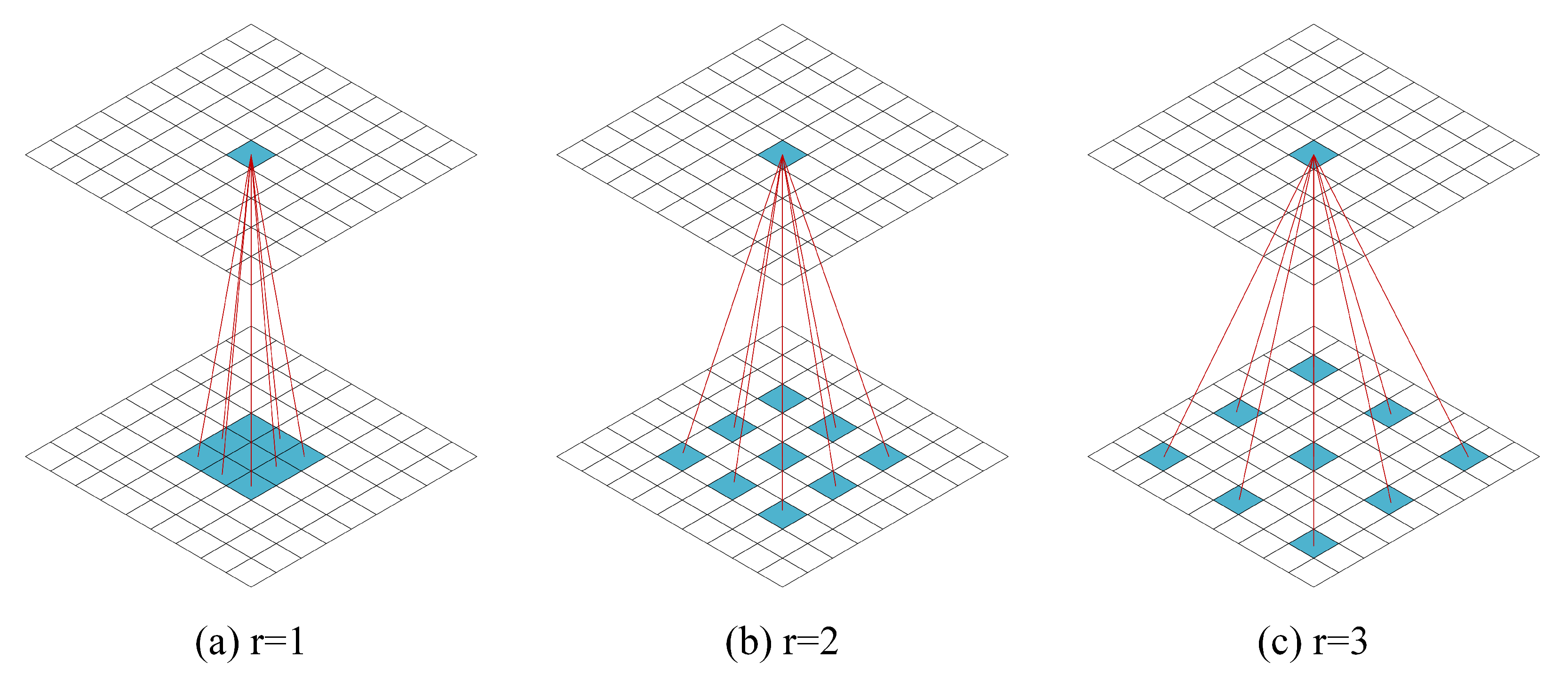
The examples of dilated convolution are shown in Figure 3. In particular, the dilated convolution expands the receptive field by inserting holes into the normal convolution, the convolution kernel is discontinuous and the features sampled are discrete and uncorrelated. The larger dilation rate will lead to more features being lost. For example, as shown in Figure 3a, the perceptual field is 3 × 3 when the dilation rate is 1, which is normal convolution, and every pixel in the perceptual field is used. When the dilation rate is 2, the receptive field is 5 × 5 , as shown in Figure 3b, and only 9 pixels are involved. When the dilation rate is 3, the field is 7 × 7 , as shown in Figure 3c. The number of pixels used is still 9. Although the dilated convolution reduces the pixels’ usage rate, it would lose more information. The identity shortcut connection between each residual block, is designed to mitigate the pixels’ loss effects.
The channel dimension is first reduced by a 3 × 3 × 512 convolution, which helps save the subsequent computational effort. The three side-by-side dilated convolutions are used to extract multi-scale features, with a dilation rate of 1, 2 and 3. The dilation rate of 1 indicates the normal convolution, which captures every detail of the image, while the convolutions with a dilation rate of 2 and 3 capture a larger field of sensation and obtain multi-scale features. By means of a constant mapping, the three extracted multi-scale features are then added to the input forming a residual structure. That allows the loss of pixel information caused by the holes to be supplemented to obtain the fused features. Each dilated convolution is followed by a ReLu activation layer. Finally, the fused features are further fused by a 3 × 3 × 512 convolution. Each module is connected to each other densely, and each layer of the module is tightly connected to the other layers behind it so that information from each layer can be passed to subsequent layers.

3.2.3. Loss Function

Euclidean loss was used to measure the estimation error between the estimated density and the supervised density. Let a set of training sample data be X i , in which i = 1 , 2 , , N . Then the density is D i p r e = M S R X i , θ . And the overall mean square error will be the Euclidean loss function as below:
L e = 1 N i = 1 N D i p r e D i g t 2 2 ,
where N is the batch size during the training. Using the Euclidean loss function to evaluate the prediction gap at the pixel level will ignore the global and local correlation between the estimated density and the true density graph. Therefore, we combined multi-scale density level consistency loss to measure Euclidean loss in both global and local contexts. The density graph is divided into sub-regions of different sizes by a pooling operation, each representing a different density level at a different location. And the network is optimised by constraint with the corresponding true value. The multi-scale density level consistency loss is defined as follows:
L c = 1 N i = 1 N j = 1 S 1 k j 2 P a v e ( D i p r e , k j ) P a v e ( D i g t , k j ) 1 ,
where S denotes the density levels of the divided density graph, P a v e denotes the average pooling level, and k j denotes the output size of the average pooling. In this work, the density graph is divided into four levels, and the average pooling output sizes are 1 × 1 , 2 × 2 , 4 × 4 and 8 × 8 . The 1 × 1 size output captures the global information while the remaining three capture the local information. The loss function is defined as follows:
L = L e + λ L c ,
where L e represents the Euclidean loss, L c is the multi-scale density level consistency loss, and λ is the weight hyperparameter that we use to balance the pixel-level and density-level losses. Algorithm 1 provides the pseudo-code of MSRNet.
Algorithm 1 Multi-scale residual cattle density estimate network (MSRNet) algorithm
Input: The input data: X t r a i n and X t e s t ;
Output: The well-trained MSRNet model F : X D ;
1:Define the model function M S R and initialize parameters θ ;
2:Define the loss function L = L e + λ L c ;
3:The data augmentation from X t r a i n to get X ^ t r a i n ;
4:for i = 1 , 2 , N do
5:for  X i X ^ t r a i n  do
6:  Calculate estimated density D i p r e = M S R ( X i , θ ) ;
7:  Calculate ground truth D i g t = H i ( X i ) · G σ ( X i ) ;
8:  Calculate the l o s s = L ( D i p r e , D i g t ) ;
9:  Update θ to minimize l o s s ;
10:end for
11:for  Y i X t e s t  do
12:  Calculate estimated density C i p r e = M S R ( Y i , θ ) ;
13:  Calculate ground truth C i g t = H i ( Y i ) · G σ ( Y i ) ;
14:end for
15: Calculate the M A E = 1 N i = 1 N | C i p r e C i g t | ;
16: Calculate the R M S E = 1 N i = 1 N | C i p r e C i g t | 2 ;
17:end for
18:Save the MSRNet model F;

3.3. Herd Image Data Collection

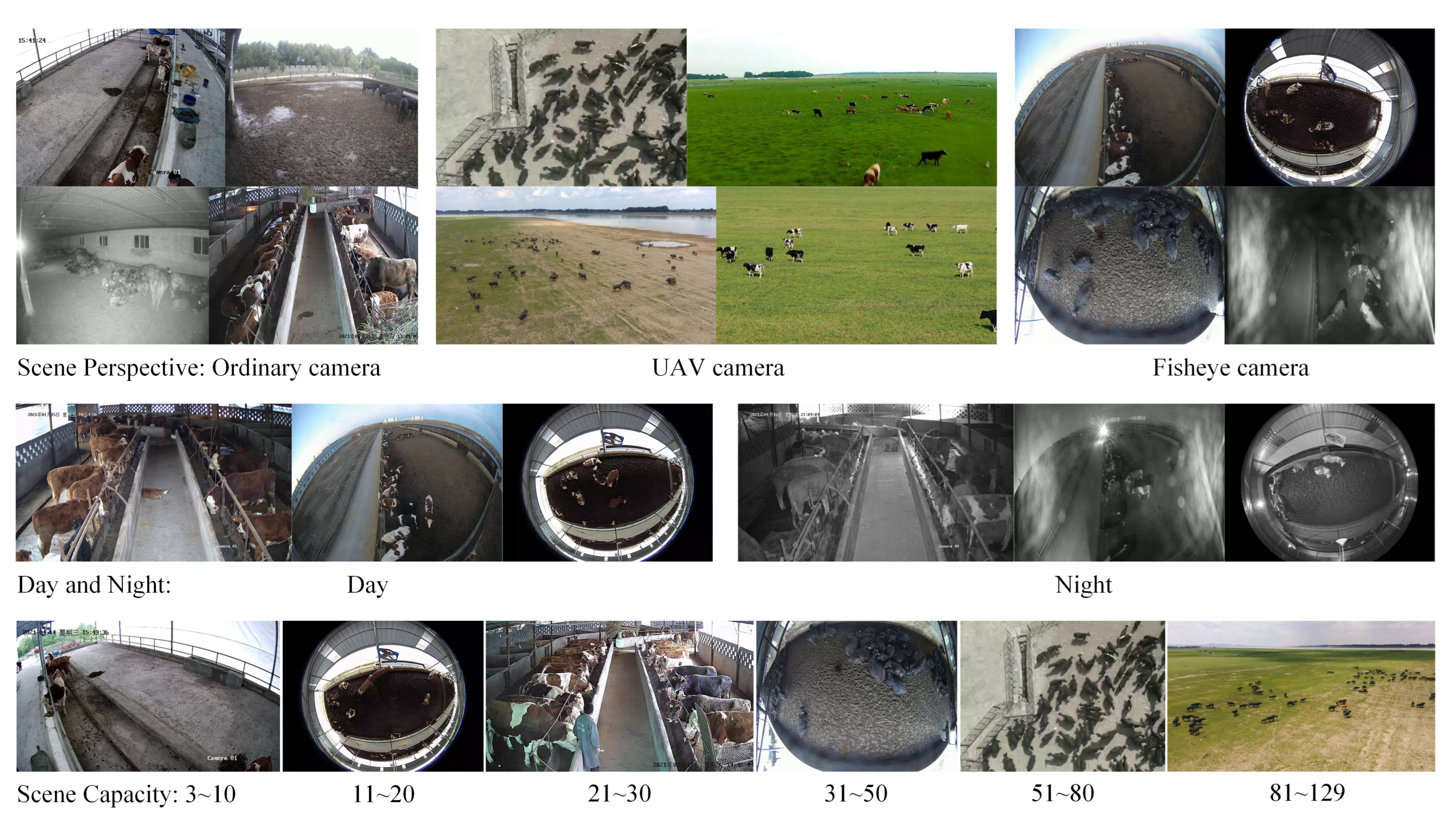
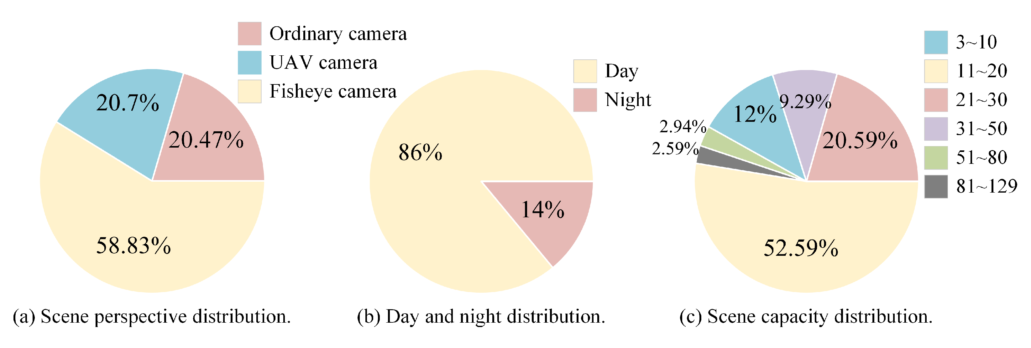
In order to evaluate our proposed MSRNet, a cattle dense dataset is also created. Our proposed dataset is large and contains a variety of scenes and lighting conditions that can represent the real situation of the pasture. Expressly, we set up smart cameras in several pastures of Yibin and Qinghai. It took five months to monitor the daily life of cattle in different periods, seasons, scenarios and weather conditions to get video data. The scenarios include indoor and outdoor cattle pens, and this research includes various types of surveillance cameras, such as fisheye cameras, ordinary cameras and UAV cameras. We intercept video data from different time periods. The intercepted surveillance videos were sampled in real-time and then selected. Data with diverse scenes and significant variations in cattle movement were picked from the dataset. All in all, 850 images were finally selected to build the density estimation dataset, which contains a total of 18,403 cattle. The number of cattle per image varies from 3 to 129 cattle. Some of these samples are shown in Figure 4. Among them, the data distribution of the above scenarios is shown in Figure 5. The fisheye cameras accounted for the largest proportion of 500 pictures, and the scene with the number of cattle in the range of 11~20 was the most, including 447 images.
Different from the crowd counting dataset labeling process, the crowd counting datasets use the head as the labeling center during the labeling process, because the position of the head in the picture is obvious and easy to distinguish. Meanwhile, the cattle herd dataset is caused by the complex perspective scene. The center of the label cannot be determined; usually it is the belly of the cow, and in the case of severe occlusion, it is the visible part of the cow, such as the head or the back of the cow. The cattle herd dataset is compared with other population datasets as shown in the Table 1.
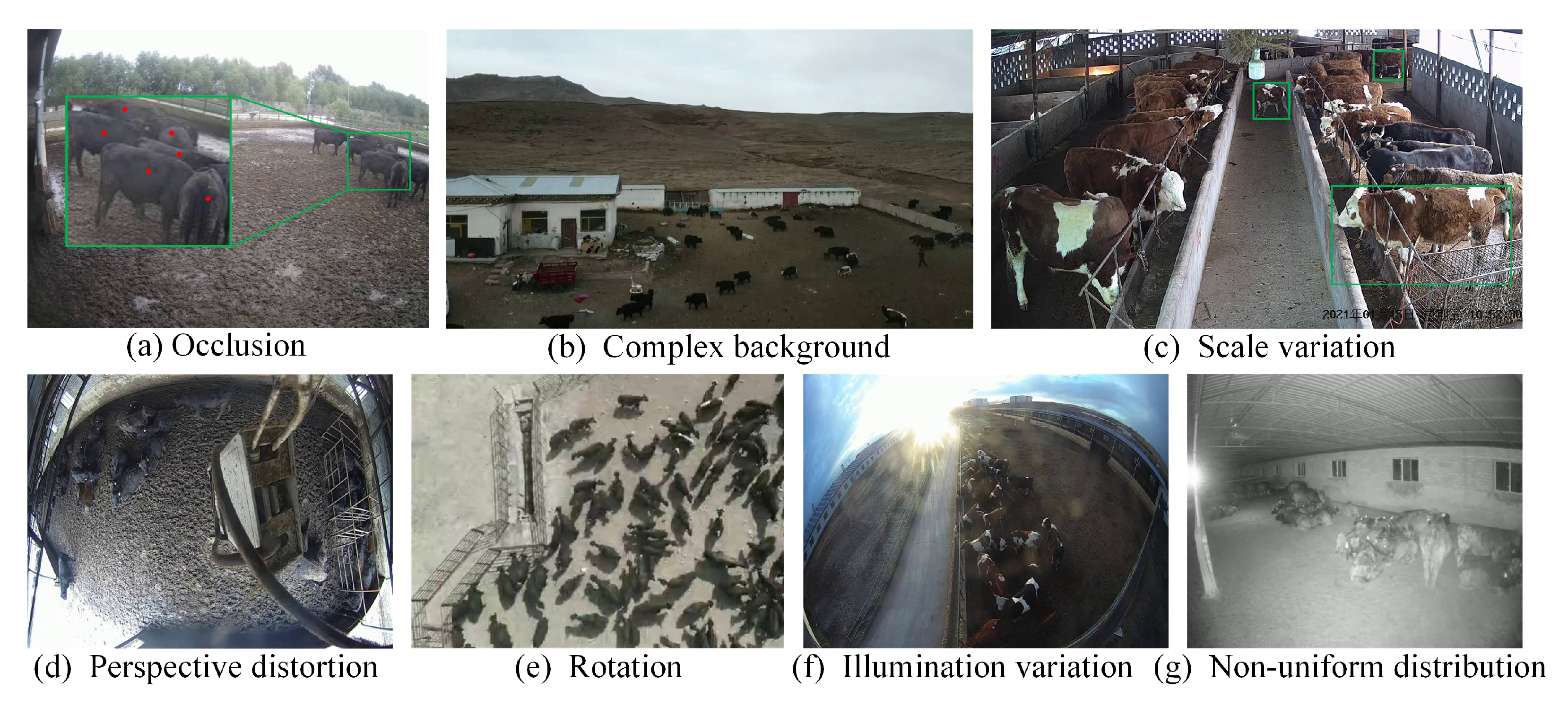
A robust network should have the capability of coping with various complex scenarios. The existence of challenges always brings many difficulties to the models, such as occlusion, complex background, scale variation, perspective distortion, rotation, illumination variation, and non-uniform distribution. Moreover, the scenes of the images are from indoor and outdoor settings, as well as in the wild. It is worth noting that these attributes are not mutually exclusive. In other words, there may exist several attributes in one image. Some samples are shown in Figure 6.

4. Experiments

4.1. Setup

We evaluate our method in two different datasets including ShanghaiTech dataset and our density estimation dataset. ShanghaiTech is a large-sized dense crowd density estimation dataset. It contains two parts: ShanghaiTech_A and ShanghaiTech_B. ShanghaiTech_A was collected randomly on the Internet with denser population distribution. ShanghaiTech_B is collected from a commercial street in Shanghai where the number of people per image is relatively sparse. The part A and B contains 482 and 716 images, respectively, and there are 330,165 people annotated in it. Our cattle density estimation dataset contains 850 images with 18,403 cattle in total. All data were divided into a training set and a testing set in a ratio of 6:4, with 493 images in the training set and 357 images in the testing set.

4.1.1. Model Training

Our fine-tuning model was based on the pre-trained VGG-16 model, with all new layers initialised by a Gaussian distribution with a mean of 0 and a standard deviation of 0.01. The learning rate was 5 × 10 6 , the weight decay rate was 5 × 10 4 and the weight hyperparameter λ was 1000. The optimisation algorithm is an adaptive moment estimation (Adam). We also adopted a set of data enhancement methods on the data during the training process. All of them are listed below:
  • Randomly cropping the image to four non-overlapping image blocks of 1/4 the size of the image, or randomly cropping one image block of 1/4 the size of the image.
  • Randomly flipping the image block, the possibility is 0.5.
  • Randomly using gamma correction on image data considering variations in illumination, the possibility is 0.3, and the parameters for gamma correction are [0.5, 1.5].

4.1.2. Evaluation Criteria

Instead of cropping the images during the testing phase, we fed the complete images into the network. They generated density graphs accordingly. Then the network is evaluated by the mean absolute error (MAE) and the root means square error (RMSE). Where the MAE can well reflect the actual situation of the error between the predicted and true values, and can be expressed by:
M A E = 1 N i = 1 N C i p r e C i g t .
The RMSE represents the expected value of the squared difference between the predicted value and the true value open square. It can evaluate the degree of change of the data. The smaller the value of the RMSE, the better the accuracy of the prediction model describing the experimental data. Its expression shows below:
R M S E = 1 N i = 1 N C i p r e C i g t 2 ,
where N represents the number of images in the test set, C i p r e represents the predicted number of cattle, and C i g t means the true number of cattle.
All the experiments were conducted on a computer with an Nvidia Geforce RTX 3090 graphics card and an AMD Ryzen 9 3900X CPU. This computer also contains two 32GB of memory working at 3600 mHz, and the operating system is CentOS7. Pytorch is adopted for implementation because it is an open-source software framework. We experimentally compared the error of the predicted cattle population with the real cattle population using target detection and density estimation methods. Because of the good model structure design and the joint loss function, the present network structure can be trained end-to-end.

4.2. Main Result

To demonstrate the effectiveness of the method in this paper, we compared the model performance on both our created cattle dataset and a benchmark dataset about population density estimation (ShanghaiTech).

4.2.1. Dataset Validity

We compared the results of all target detection methods, including density estimation methods MCNN [7], CSRNet [8] and DSNet [9]. All the experiments are based on the cattle population dataset. In particular, we set the same parameter for the density estimation model. The MAE and RMSE metrics were also utilized to evaluate the counting accuracy and the model’s robustness.
We demonstrate some of the prediction results of each model on the cattle dataset in Figure 7. The first column is the original image data. The second column shows the true value of the density graph. The third column is the density graph predicted by our MSRNet, and the following columns are the density graph predicted by MCNN, CSRNet, and DSNet, respectively. According to the prediction results, the prediction results of our MSRNet are relatively close to the true values in all scenarios above. In terms of the distribution of the predicted densities, MSRNet shows better performance to match the distribution of the real density graph. In contrast, the MCNN is more easily disturbed by the background and will identify some background information as cattle by mistake, especially in the scene of the fisheye indoor camera, which will misidentify the cattle pen wall as cattle. CSRNet cannot distinguish well between cattle and background for the night and the highly overlapping situation, which means the robustness of the model is limited. The individual differentiation of the predicted density graph proved that our MSRNet has a clearer boundary differentiation for sparse scenes, even in the less differentiated black cattle groups. In contrast, DSNet shows very unclear boundary information in black bull scenes. All in all, the MSRNet proposed in this paper provides the most accurate prediction results, and the predicted density distribution is closer to the ground truth. The adaptability to various scenes is better compared with other methods. The boundary can be more clearly distinguished for sparse scenes, and the background’s anti-interference ability is better.
The evaluation results of MAE and RMSE on the cattle dataset are listed in Table 2. Compared to other methods, MSRNet achieved the lowest value on both MAE and RMSE. It even shows a drop of about 12.2% in MAE and 14.2% in RMSE compared to DSNet, which shows the second-best performance. In the cattle targets overlap scenario, the targets detection method can cause many misdetections. MCNN learns features of different sizes through three different convolution channels. CSRNet utilizes dilated convolution at the back end of the network to keep the resolution of features constant but cannot adapt to large scale variations problems. DSNet uses densely connected dilated convolution to maintain continuous information transfer as well as multi-scale feature extraction. However, the overly dense connections tend to lead to overfitting. As only a very small percentage of training data contains 50~100 cattle, there is an accuracy plummet for DSNet on them. In contrast, MSRNet achieves the best performance in both MAE and RMSE by extracting multi-scale features and adapting to the scale variation of the cattle population while using residuals to resolve the grid effect brought about by the dilated convolution and compensate for the lost pixel feature information. This experiment demonstrates that the MSRNet can accurately count the cattle number in a cattle farm, with an overall average error of around 1.85.

4.2.2. Validity Test on ShanghaiTech Datasets

MSRNet not only predicts density better on cattle dataset but also achieves better results in human population density estimation. The experimental results on these datasets are shown in Table 3. MSRNet achieved the best performance according to MAE and RMSE values on ShanghaiTech_A. We guess that in contrast to traditional crowd density estimation, crowd datasets are usually labeled with the heads of people, while cattle datasets are labeled with the body of cattle, and ShanghaiTech_B is sparser than ShanghaiTech_A, in which the occlusion and scale changes of people are smaller, so it only achieved sub-optimal performance in the ShanghaiTech_B. This experiment proves that MSRNet is highly adaptive and robust and can have good prediction results for completely different scenarios and targets.

4.2.3. Ablation Experiments

We discuss the result of ablation experiments conducted to analyse the effect of different components in MSRNet as well as weight of the multi-scale density level consistency loss. Due to the presence of various complexities such as high density occlusion and complex background, we perform the ablation experiments on the proposed cattle dataset.
We conduct the first ten convolutional layers and three pooling layers of the conventional VGG-16 network as the backbone, and connect the last three convolutional layers to be the base network. Then we add components incrementally such as the MSR block and multi-scale density level consistency loss. Meanwhile, we try to use ResNet-50 [30] as the backbone to extract a feature to observe whether it receives a better performance. All the results of experiments are shown in Table 4. The VGG-16 with last three convolutional layers as the base network achieves an MAE of 5.34. By adding the proposed MSR and multi-scale density level consistency loss incrementally to enrich the base network, the MAE decreases to 1.85, which improved by a big margin and achieves the best performance compared with previous methods. When we try to replace the backbone network, such as the first 22 convolutional layers and the interlacing pooling layer of the ResNet-50 for the experiment, however, we do not receive the expected results and only achieve an MAE of 8.64. The possible reason for this is that ResNet is proposed to solve the depth problem of the convolutional neural network when dealing with large datasets, but the proposed cattle dataset is less than the common public datasets, so there is a serious effect of overfitting.
In addition, we set the different values of weight in Equation (5) to analyse the influence on the experiments and the results are shown in Table 5. Before we add the multi-scale density level consistency loss, the proposed network only achieves an MAE of 5.10. After we add the the consistency loss and set the value of weight to 10, the MAE decreases to 2.02. As we increase the weight value gradually, the result shows the best performance of MAE of 1.85 when the value of weight is 1000. However, as we continue to increase the value of weight to 10,000, the MAE goes up instead of down.

4.3. Discussion

This paper proposed a multi-scale residual cattle density estimate network to address the problems of the large scale variation of cattle. We chose VGG-16 as the backbone network to extract features and select MSR blocks for feature fusion. However, without scale annotations, it is sub-optimal and error-prone to manually assign the predictions for heads of different scales to specific feature levels. Song et al. [31] proposed a patch-wise feature level selection strategy to identify the most appropriate feature level. Such a novel strategy effectively exploits the multi-scale feature representations inside a multi-level network, offering a new way to address the large challenging scale variation problem. We wonder if it is possible to further fuse the multi-scale features of the backbone network to identify the most suitable feature level for each scale, perhaps to achieve better results. Introducing the geometrics method such as equivariant GNN and CNN also shows potential. Cohen et al. [32] proposed an equivariant GNN for image rotation and Lagrave et al. [33] demonstrated equivariant CNN in fish-eye image processing. We may try these approaches in future research.

5. Conclusions

This paper first collected a cattle density estimation dataset and summarised the task as uneven distribution, scale variation and grid effect. We proposed a multi-scale residual cattle density estimation network to address them. The MSRNet model uses dilated convolution with different dilation rates to obtain multi-scale features. The residual structure to solve the problem of grid effect is caused by using dilated convolution. Experiments show that the proposed method is more effective and accurate than traditional methods for estimating herd density, with better model robustness. There is still potential improvement in the estimation of the cattle, such as the generated supervised information. Since the objective of human crowd density estimation is different from that of cattle density estimation, using the traditional Gaussian kernel to generate the supervised information is not suitable for cattle, mainly because crowds are usually labelled with human heads. In contrast, the shape of individual cattle is very different from that of human heads. Subsequent improvements will be made in the direction of annotated information generation.

Author Contributions

Conceptualization, Y.T.; Data curation, M.Z.; Formal analysis, M.Z.; Funding acquisition, Y.T.; Investigation, M.Z.; Methodology, M.Z.; Project administration, M.Z.; Resources, Y.T.; Software, M.Z.; Supervision, Y.T.; Validation, H.Z. and S.Y.; Visualization, M.Z.; Writing—original draft, M.Z.; Writing—review and editing, J.L. All authors have read and agreed to the published version of the manuscript.

Funding

This research received no external funding.

Data Availability Statement

The cattle dataset is available at https://github.com/menjure/Cattle-dataset.

Conflicts of Interest

The authors declare no conflict of interest.

References

  1. Kamilaris, A.; Prenafeta-Boldú, F.X. Deep learning in agriculture: A survey. Comput. Electron. Agric. 2018, 147, 70–90. [Google Scholar] [CrossRef] [Green Version]
  2. Ryan, D.; Denman, S.; Fookes, C.; Sridharan, S. Scene invariant multi camera crowd counting. Pattern Recognit. Lett. 2014, 44, 98–112. [Google Scholar] [CrossRef] [Green Version]
  3. Sang, J.; Wu, W.; Luo, H.; Xiang, H.; Zhang, Q.; Hu, H.; Xia, X. Improved crowd counting method based on scale-adaptive convolutional neural network. IEEE Access 2019, 7, 24411–24419. [Google Scholar] [CrossRef]
  4. Fu, H.; Ma, H.; Xiao, H. Scene-adaptive accurate and fast vertical crowd counting via joint using depth and color information. Multimed. Tools Appl. 2014, 73, 273–289. [Google Scholar] [CrossRef]
  5. Zhang, G. Current status and trends in the development of smart animal husbandry. China Status Quo 2019, 12, 33–35. [Google Scholar]
  6. Idrees, H.; Saleemi, I.; Seibert, C.; Shah, M. Multi-source multi-scale counting in extremely dense crowd images. In Proceedings of the IEEE Conference on Computer Vision and Pattern Recognition, Portland, OR, USA, 23–28 June 2013; pp. 2547–2554. [Google Scholar]
  7. Zhang, Y.; Zhou, D.; Chen, S.; Gao, S.; Ma, Y. Single-image crowd counting via multi-column convolutional neural network. In Proceedings of the IEEE Conference on Computer Vision and Pattern Recognition, Las Vegas, NV, USA, 26 June–1 July 2016; pp. 589–597. [Google Scholar]
  8. Li, Y.; Zhang, X.; Chen, D. Csrnet: Dilated convolutional neural networks for understanding the highly congested scenes. In Proceedings of the IEEE Conference on Computer Vision and Pattern Recognition, Salt Lake City, UT, USA, 18–23 June 2018; pp. 1091–1100. [Google Scholar]
  9. Dai, F.; Liu, H.; Ma, Y.; Zhang, X.; Zhao, Q. Dense scale network for crowd counting. In Proceedings of the 2021 International Conference on Multimedia Retrieval, Taipei, Taiwan, 21–24 August 2021; pp. 64–72. [Google Scholar]
  10. Shen, Z.; Xu, Y.; Ni, B.; Wang, M.; Hu, J.; Yang, X. Crowd counting via adversarial cross-scale consistency pursuit. In Proceedings of the IEEE Conference on Computer Vision and Pattern Recognition, Salt Lake City, UT, USA, 18–23 June 2018; pp. 5245–5254. [Google Scholar]
  11. Cao, X.; Wang, Z.; Zhao, Y.; Su, F. Scale aggregation network for accurate and efficient crowd counting. In Proceedings of the European Conference on Computer Vision (ECCV), Munich, Germany, 8–14 September 2018; pp. 734–750. [Google Scholar]
  12. Huang, Z.; Li, Y. Contextual multiscale fusion-based algorithm for cotton boll counting. Appl. Res. Comput. 2021, 6, 1913–1916. [Google Scholar]
  13. Lu, H.; Cao, Z.; Xiao, Y.; Zhuang, B.; Shen, C. TasselNet: Counting maize tassels in the wild via local counts regression network. Plant Methods 2017, 13, 1–17. [Google Scholar] [CrossRef] [PubMed] [Green Version]
  14. Liu, X. Deep Learning-Based Method for Automatic Cell Counting in Fluorescence Microscopy Imaging. Ph.D. Thesis, University of Electronic Science and Technology, Chengdu, China, 2020. [Google Scholar]
  15. Ma, Z.; Yu, L.; Chan, A.B. Small instance detection by integer programming on object density maps. In Proceedings of the IEEE Conference on Computer Vision and Pattern Recognition, Boston, MA, USA, 7–12 June 2015; pp. 3689–3697. [Google Scholar]
  16. Sindagi, V.A.; Patel, V.M. A survey of recent advances in cnn-based single image crowd counting and density estimation. Pattern Recognit. Lett. 2018, 107, 3–16. [Google Scholar] [CrossRef] [Green Version]
  17. Cheng, D.; Rong, T.; Cao, G. Density map estimation for crowded chicken. In Proceedings of the International Conference on Image and Graphics, Beijing, China, 23–25 August 2019; Springer: Berlin/Heidelberg, Germany, 2019; pp. 432–441. [Google Scholar]
  18. Hobbs, J.; Paull, R.; Markowicz, B.; Rose, G. Flowering density estimation from aerial imagery for automated pineapple flower counting. In Proceedings of the AI for Social Good Workshop, Virtual, 20–21 July 2020. [Google Scholar]
  19. Johnston, A.; Edwards, D. Welfare implications of identification of cattle by ear tags. Vet. Rec. 1996, 138, 612–614. [Google Scholar] [CrossRef] [PubMed]
  20. Xu, B.; Wang, W.; Falzon, G.; Kwan, P.; Schneider, D. Automated cattle counting using Mask R-CNN in quadcopter vision system. Comput. Electron. Agric. 2020, 171, 105300. [Google Scholar] [CrossRef]
  21. Li, Q.; Shang, J.; Li, B. Automatic counting method for grassland sheep based on head image features. China Meas. Test 2020, 46, 5. [Google Scholar]
  22. Lowe, D.G. Object recognition from local scale-invariant features. In Proceedings of the Seventh IEEE International Conference on Computer Vision, Corfu, Greece, 20–25 September 1999; Volume 2, pp. 1150–1157. [Google Scholar]
  23. Tian, M.; Guo, H.; Chen, H.; Wang, Q.; Long, C.; Ma, Y. Automated pig counting using deep learning. Comput. Electron. Agric. 2019, 163, 104840. [Google Scholar] [CrossRef]
  24. Wan, J.; Wang, Q.; Chan, A.B. Kernel-based density map generation for dense object counting. IEEE Trans. Pattern Anal. Mach. Intell. 2020, 44, 1357–1370. [Google Scholar] [CrossRef] [PubMed]
  25. Chan, A.; Vasconcelos, N. Ucsd pedestrian dataset. IEEE Trans. Pattern Anal. Mach. Intell. (TPAMI) 2008, 30, 909–926. [Google Scholar] [CrossRef] [PubMed] [Green Version]
  26. Zhang, C.; Li, H.; Wang, X.; Yang, X. Cross-scene crowd counting via deep convolutional neural networks. In Proceedings of the IEEE Conference on Computer Vision and Pattern Recognition, Boston, MA, USA, 7–12 June 2015; pp. 833–841. [Google Scholar]
  27. Shao, W.; Kawakami, R.; Yoshihashi, R.; You, S.; Kawase, H.; Naemura, T. Cattle detection and counting in UAV images based on convolutional neural networks. Int. J. Remote. Sens. 2020, 41, 31–52. [Google Scholar] [CrossRef]
  28. Simonyan, K.; Zisserman, A. Very deep convolutional networks for large-scale image recognition. arXiv 2014, arXiv:1409.1556. [Google Scholar]
  29. Yu, F.; Koltun, V. Multi-scale context aggregation by dilated convolutions. arXiv 2015, arXiv:1511.07122. [Google Scholar]
  30. He, K.; Zhang, X.; Ren, S.; Sun, J. Deep Residual Learning for Image Recognition. In Proceedings of the IEEE Conference on Computer Vision and Pattern Recognition (CVPR), Las Vegas, NV, USA, 27–30 June 2016. [Google Scholar]
  31. Song, Q.; Wang, C.; Wang, Y.; Tai, Y.; Wang, C.; Li, J.; Wu, J.; Ma, J. To choose or to fuse? Scale selection for crowd counting. In Proceedings of the AAAI Conference on Artificial Intelligence, Virtual, 2–9 February 2021; Volume 35, pp. 2576–2583. [Google Scholar]
  32. Cohen, T.; Welling, M. Group equivariant convolutional networks. In Proceedings of the International Conference on Machine Learning, PMLR, New York, NY, USA, 20–22 June 2016; pp. 2990–2999. [Google Scholar]
  33. Lagrave, P.Y.; Barbaresco, F. Hyperbolic Equivariant Convolutional Neural Networks for Fish-Eye Image Processing. Available online: https://hal.archives-ouvertes.fr/hal-03553274 (accessed on 25 February 2022).
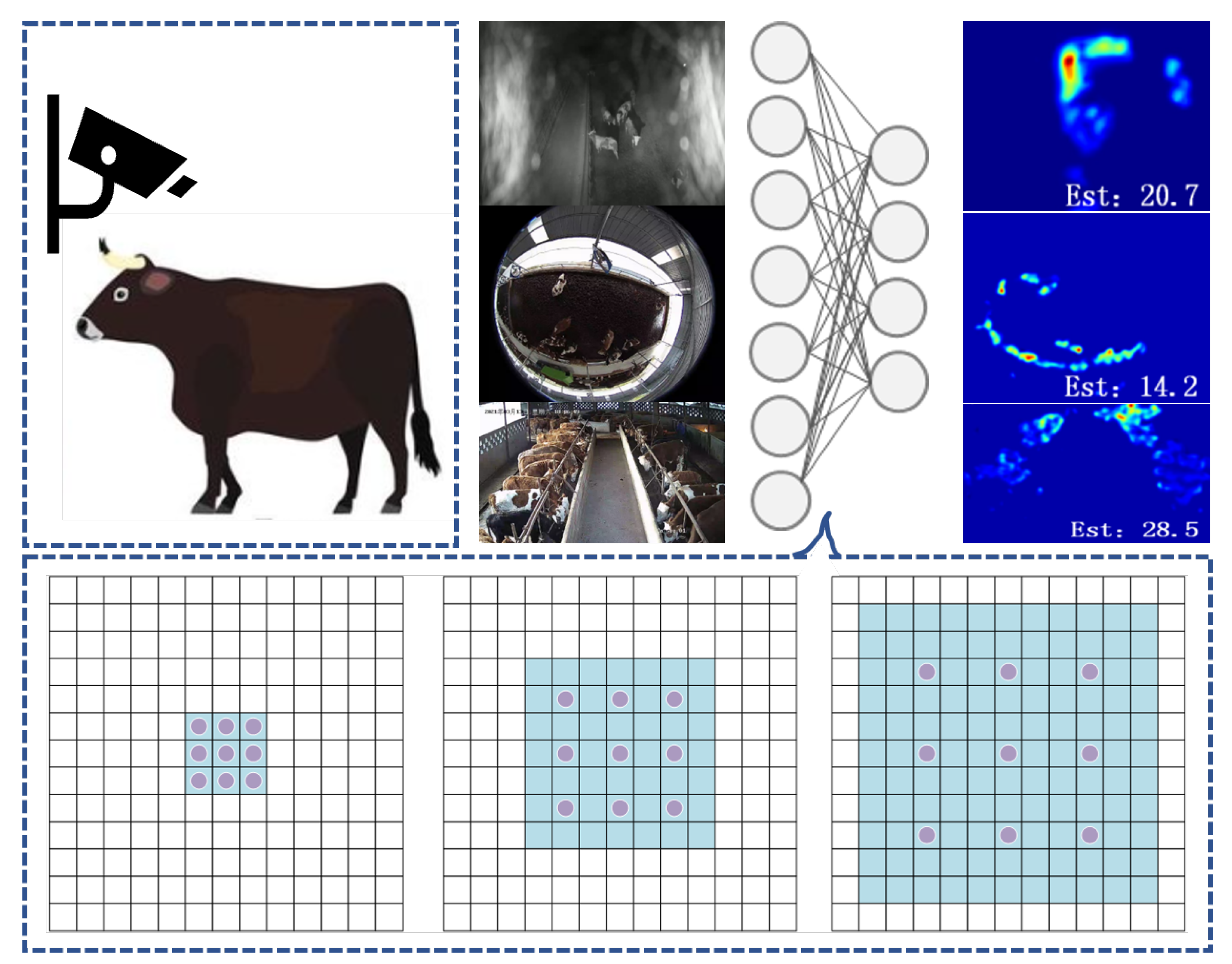
Figure 1. Given a conceptual description from data collection to model training, in which the module obtains multi-scale receptive fields by using multi-column dilated convolution to handle the problem of scale variations of cattle.
Mathematics 10 03856 g001
Figure 2. An illustration of our framework of MSRNet.
Mathematics 10 03856 g002
Figure 3. Dilated convolution receptive fields with different rates.
Mathematics 10 03856 g003
Figure 4. Representative samples of the images in the collected pasture dataset.
Mathematics 10 03856 g004
Figure 5. The data distribution of the above scenarios.
Mathematics 10 03856 g005
Figure 6. The examples of challenges in cattle counting.
Mathematics 10 03856 g006
Figure 7. Density prediction results of different scenarios.
Mathematics 10 03856 g007
Table 1. Statistics of different crowd counting datasets and cattle counting dataset.
DatasetNumber of ImagesAverage ResolutionCount Statistics
TotalMinAveMax
UCSD [25]2000158 × 23849,885112546
UCF_CC_50 [6]502101 × 288863,9749412794543
WorldExpo [26]3980576 × 720199,923150253
ShanghaiTech_A [7]482589 × 868241,677335013139
ShanghaiTech_B [7]716768 × 102488,4889123578
Cattle dataset850864 × 131718,403322129
Table 2. Estimation errors on the cattle dataset.
ModelsMAERMSE
MCNN [7]6.5710.25
CSRet [8]11.5714.61
DSNet [9]2.143.31
MSRNet1.852.64
Table 3. Estimation error on the ShanghaiTech datasets.
ModelsShanghaiTech_AShanghaiTech_B
MAERMSEMAERMSE
MCNN [7]110.2173.226.433.4
ACSCP [10]75.7102.717.227.4
CSRNet [8]68.2115.010.616.0
SANet [11]67.0104.58.413.6
KDMG [24]63.899.27.812.7
MSRNet63.596.88.413.0
Table 4. Estimation errors for different components.
MethodMAERMSE
VGG-165.348.86
VGG-16 + MSR5.107.20
VGG-16 + MSR + L c 1.852.64
ResNet-50 + MSR + L c 8.6412.65
Table 5. Estimation errors for different values of weight.
Value of WeightMAERMSE
λ = 0 (w/o L c )5.107.20
λ = 102.022.88
λ = 1001.872.84
λ = 10001.852.64
λ = 10,0001.902.81
Publisher’s Note: MDPI stays neutral with regard to jurisdictional claims in published maps and institutional affiliations.