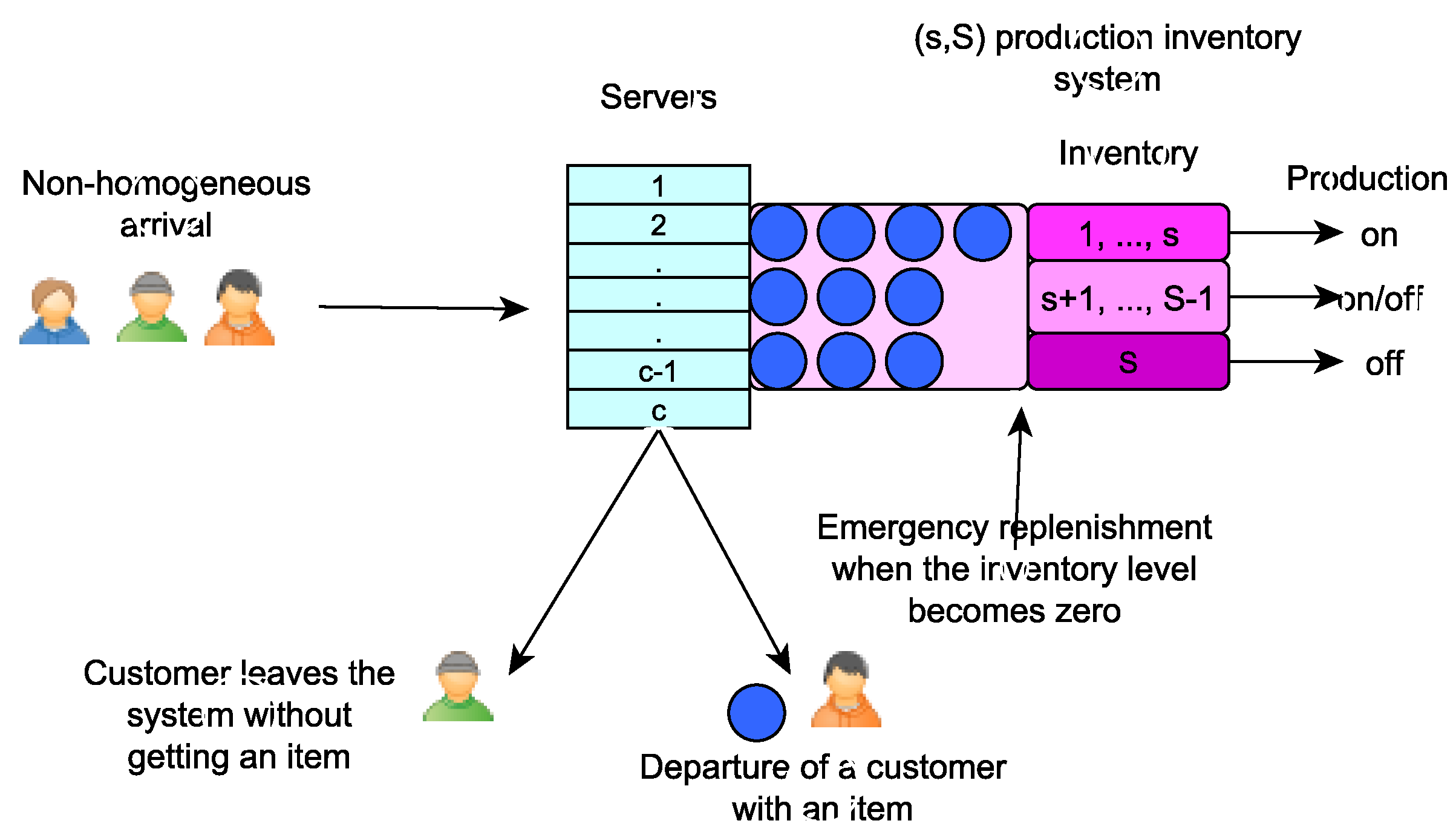
Figure 1.
Picture representation of the model.
Figure 1.
Picture representation of the model.
Figure 2.
Effect on .
Figure 2.
Effect on .
Figure 3.
Effect on .
Figure 3.
Effect on .
Figure 4.
Effect on .
Figure 4.
Effect on .
Figure 5.
Effect on .
Figure 5.
Effect on .
Figure 6.
Effect on .
Figure 6.
Effect on .
Figure 7.
Effect on .
Figure 7.
Effect on .
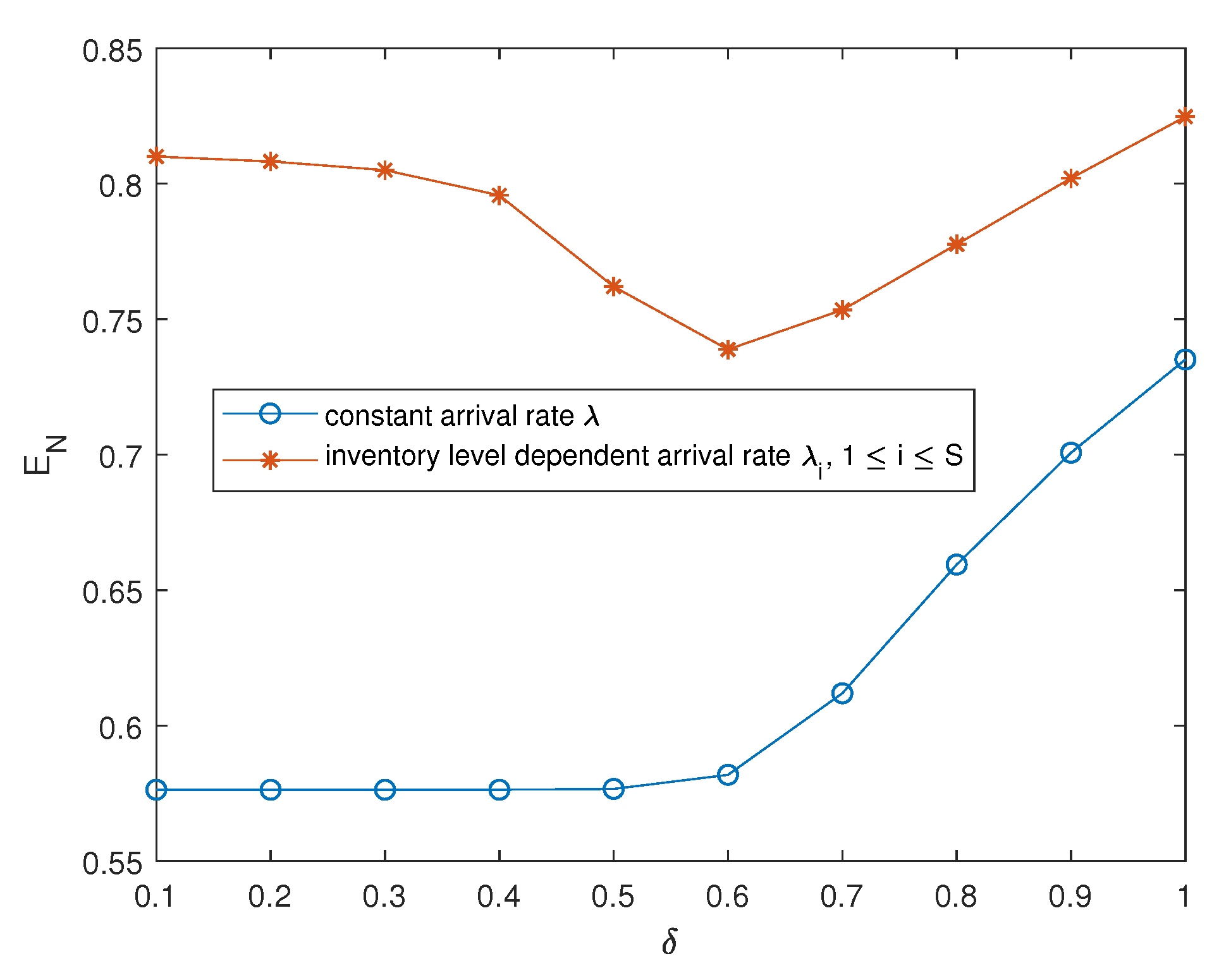
Figure 8.
Effect of on .
Figure 8.
Effect of on .
Figure 9.
Effect of on .
Figure 9.
Effect of on .
Table 1.
Effect of for .
Table 1.
Effect of for .
| | | | | | |
|---|
| 1 | 0.1949 | 23.2314 | 1.0913 | 0.0315 | 0.1949 | 0.0001 |
| 1.5 | 0.2912 | 22.4978 | 1.6307 | 0.0291 | 0.2912 | 0.0002 |
| 2 | 0.3840 | 20.5180 | 2.1476 | 0.0173 | 0.3838 | 0.0003 |
| 2.5 | 0.4611 | 14.2006 | 2.5228 | 0.0035 | 0.4576 | 0.0071 |
| 3 | 0.5341 | 6.9958 | 2.5974 | 0.0007 | 0.5065 | 0.0425 |
| 3.5 | 0.6433 | 4.3116 | 2.5981 | 0.0002 | 0.5630 | 0.0975 |
Table 2.
Effect of for .
Table 2.
Effect of for .
| | | | | | |
|---|
| 5 | 2.5101 | 6.0240 | 2.4648 | 0.0171 | 1.2564 | 0.3058 |
| 6 | 2.0056 | 4.7143 | 2.5076 | 0.0133 | 1.0498 | 0.3308 |
| 7 | 1.6307 | 3.6792 | 2.5411 | 0.0093 | 0.8999 | 0.3365 |
| 8 | 1.3458 | 2.9702 | 2.5641 | 0.0061 | 0.7871 | 0.3271 |
| 9 | 1.1296 | 2.5288 | 2.5785 | 0.0038 | 0.6995 | 0.3094 |
| 10 | 0.9651 | 2.2678 | 2.5871 | 0.0024 | 0.6295 | 0.2888 |
Table 3.
Effect of for .
Table 3.
Effect of for .
| | | | | | |
|---|
| 1.4 | 1.2910 | 4.1961 | 1.3475 | 0.0154 | 0.7459 | 0.3420 |
| 1.6 | 1.2559 | 4.2002 | 1.5435 | 0.0145 | 0.7498 | 0.3216 |
| 1.8 | 1.2223 | 4.2163 | 1.7404 | 0.0136 | 0.7539 | 0.3011 |
| 2 | 1.1899 | 4.2468 | 1.9380 | 0.0127 | 0.7582 | 0.2805 |
| 2.2 | 1.1590 | 4.2949 | 2.1364 | 0.0118 | 0.7628 | 0.2598 |
| 2.4 | 1.1294 | 4.3647 | 2.3354 | 0.0109 | 0.7678 | 0.2390 |
Table 4.
Effect of for .
Table 4.
Effect of for .
| | | | | | |
|---|
| 0.1 | 0.8100 | 27.7074 | 0.5731 | 0.0267 | 0.7918 | 0.0001 |
| 0.2 | 0.8082 | 27.1839 | 1.1214 | 0.0250 | 0.7902 | 0.0001 |
| 0.3 | 0.8050 | 26.3072 | 1.6633 | 0.0241 | 0.7873 | 0.0003 |
| 0.4 | 0.7957 | 23.9226 | 2.1781 | 0.0148 | 0.7783 | 0.0004 |
| 0.5 | 0.7620 | 15.9770 | 2.5265 | 0.0037 | 0.7393 | 0.0087 |
| 0.6 | 0.7388 | 8.0777 | 2.5752 | 0.0020 | 0.6814 | 0.0481 |
| 0.7 | 0.7534 | 5.4415 | 2.5717 | 0.0028 | 0.6504 | 0.0969 |
| 0.8 | 0.7776 | 4.3754 | 2.5681 | 0.0037 | 0.6331 | 0.1403 |
| 0.9 | 0.8020 | 3.8054 | 2.5659 | 0.0044 | 0.6219 | 0.1770 |
| 1 | 0.8247 | 3.4446 | 2.5647 | 0.0051 | 0.6139 | 0.2079 |
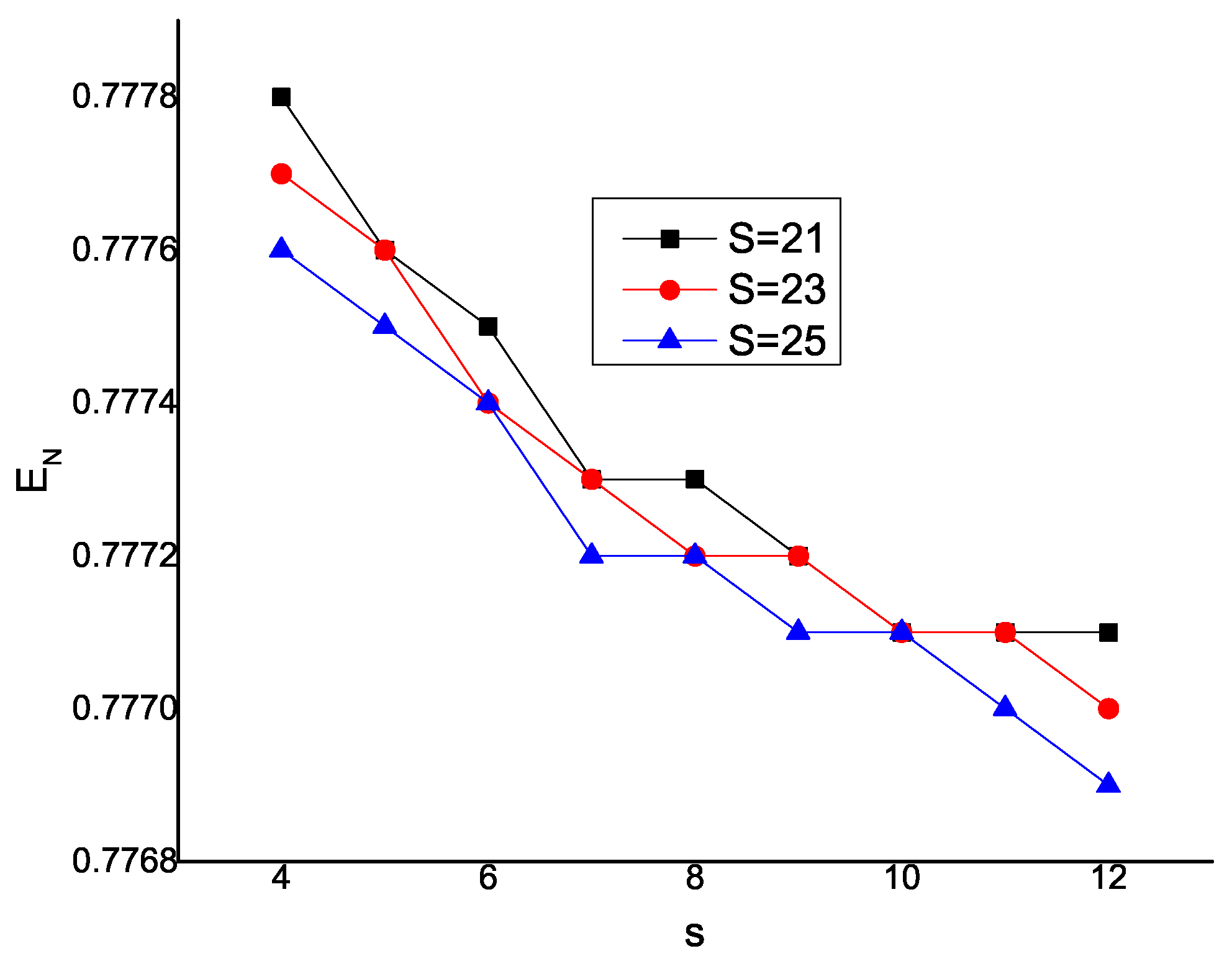
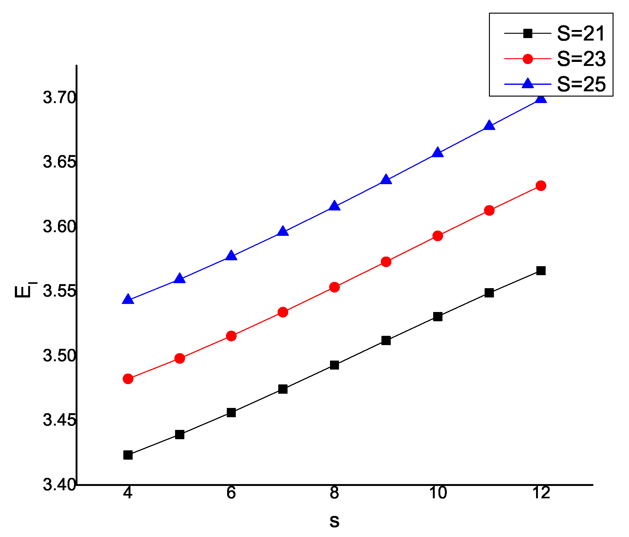
Table 5.
Effect of s and S for .
Table 5.
Effect of s and S for .
| Effect on | Effect on |
|---|
| | | | | | | |
| 4 | 0.7778 | 0.7777 | 0.7776 | 4 | 3.4233 | 3.4822 | 3.5432 |
| 5 | 0.7776 | 0.7776 | 0.7775 | 5 | 3.4391 | 3.4981 | 3.5593 |
| 6 | 0.7775 | 0.7774 | 0.7774 | 6 | 3.4561 | 3.5154 | 3.577 |
| 7 | 0.7773 | 0.7773 | 0.7772 | 7 | 3.4742 | 3.5339 | 3.5958 |
| 8 | 0.7773 | 0.7772 | 0.7772 | 8 | 3.4929 | 3.5532 | 3.6156 |
| 9 | 0.7772 | 0.7772 | 0.7771 | 9 | 3.5118 | 3.573 | 3.6361 |
| 10 | 0.7771 | 0.7771 | 0.7771 | 10 | 3.5306 | 3.593 | 3.657 |
| 11 | 0.7771 | 0.7771 | 0.7770 | 11 | 3.5489 | 3.6128 | 3.678 |
| 12 | 0.7771 | 0.7770 | 0.7769 | 12 | 3.566 | 3.632 | 3.6989 |
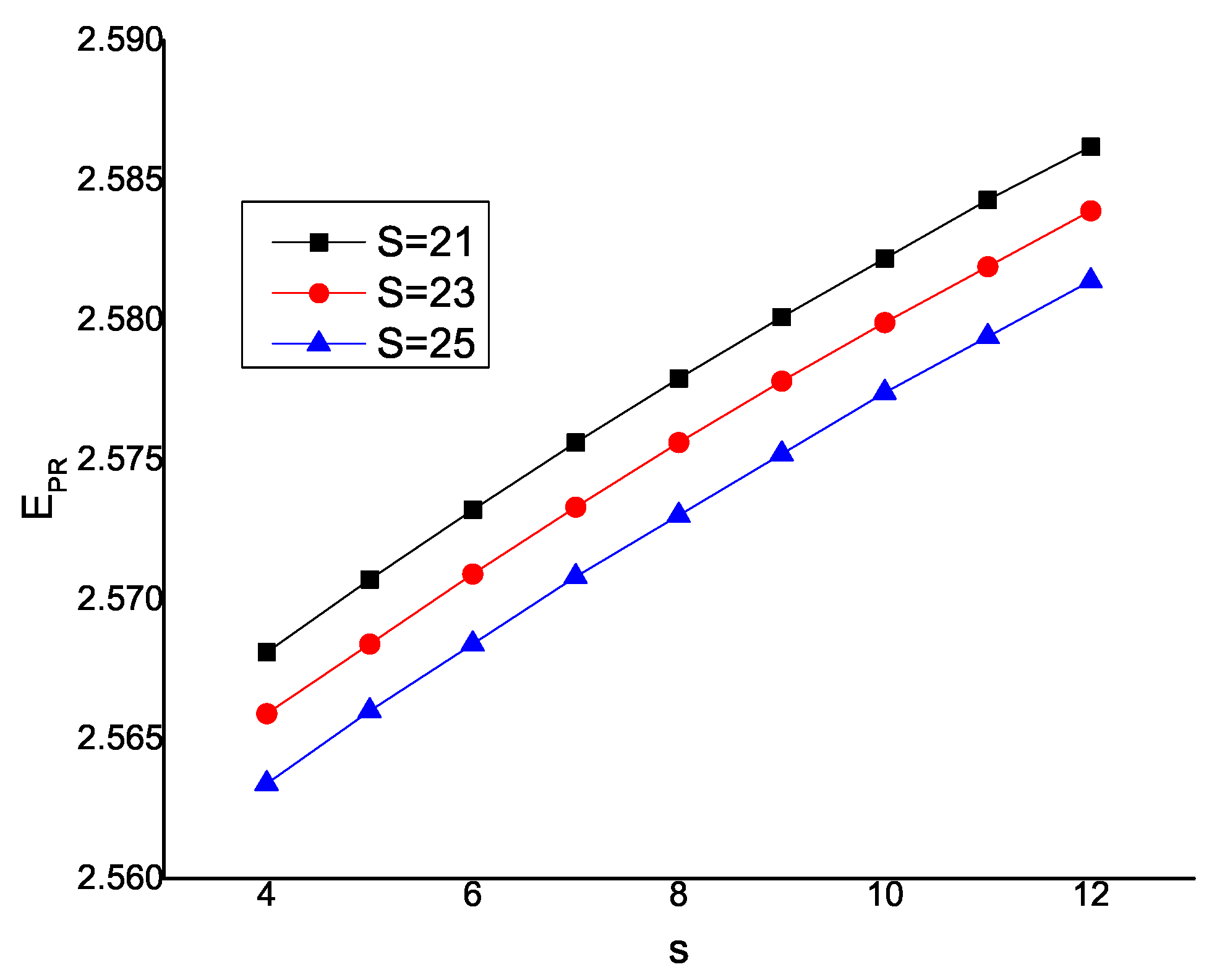
Table 6.
Effect of s and S for .
Table 6.
Effect of s and S for .
| Effect on | Effect on |
|---|
| | | | | | | |
| 4 | 2.5681 | 2.5659 | 2.5634 | 4 | 0.0042 | 0.0041 | 0.004 |
| 5 | 2.5707 | 2.5684 | 2.566 | 5 | 0.0041 | 0.004 | 0.0039 |
| 6 | 2.5732 | 2.5709 | 2.5684 | 6 | 0.004 | 0.0039 | 0.0038 |
| 7 | 2.5756 | 2.5733 | 2.5708 | 7 | 0.0039 | 0.0038 | 0.0037 |
| 8 | 2.5779 | 2.5756 | 2.573 | 8 | 0.0038 | 0.0037 | 0.0036 |
| 9 | 2.5801 | 2.5778 | 2.5752 | 9 | 0.0037 | 0.0036 | 0.0035 |
| 10 | 2.5822 | 2.5799 | 2.5774 | 10 | 0.0036 | 0.0035 | 0.0034 |
| 11 | 2.5843 | 2.5819 | 2.5794 | 11 | 0.0035 | 0.0034 | 0.0033 |
| 12 | 2.5862 | 2.5839 | 2.5814 | 12 | 0.0034 | 0.0033 | 0.0032 |
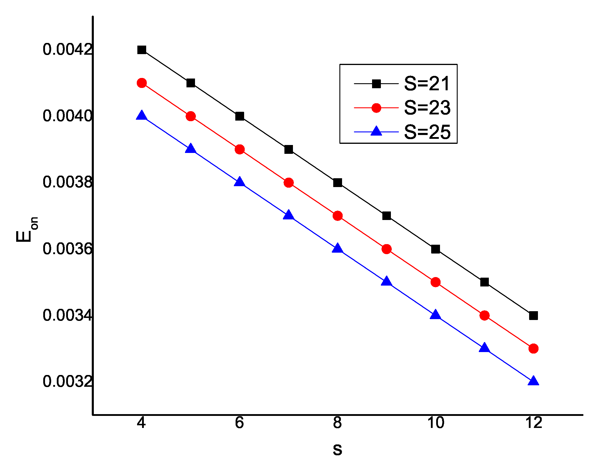
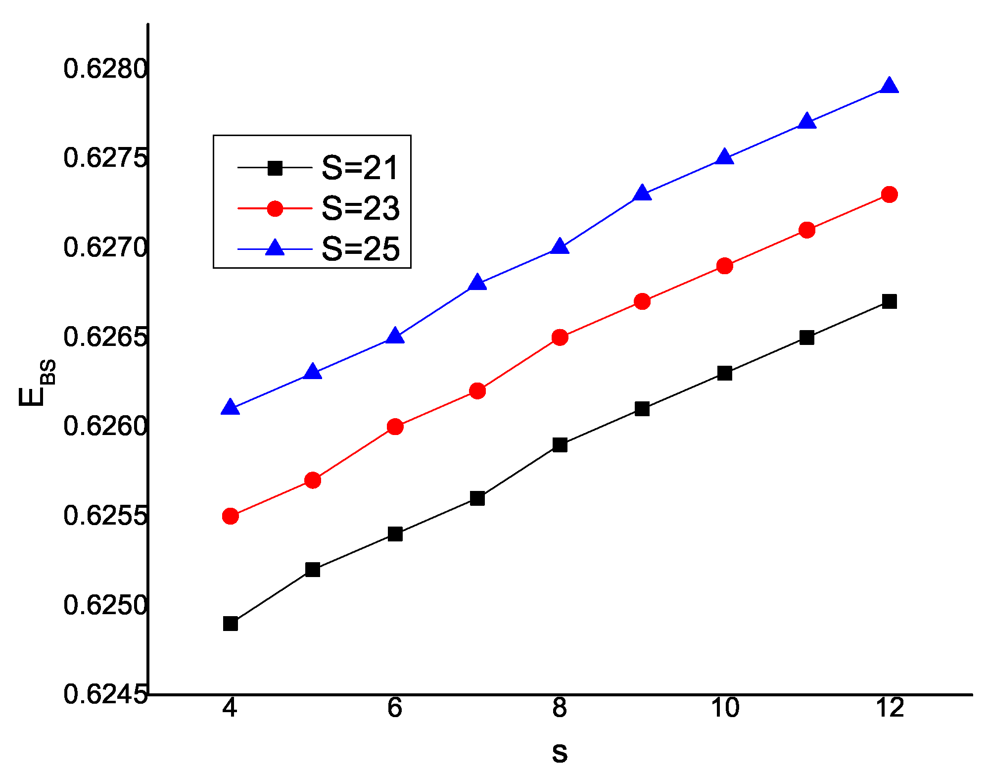
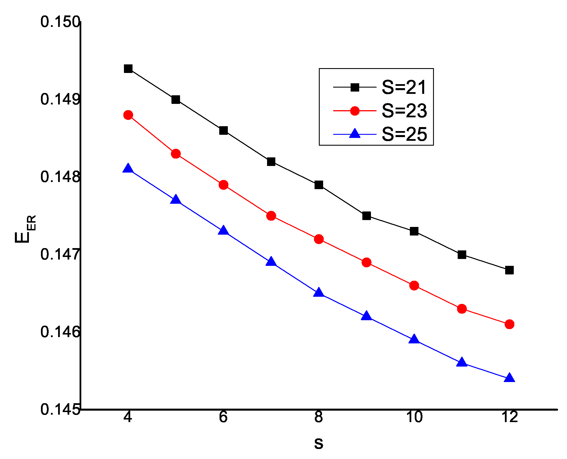
Table 7.
Effect of s and S for .
Table 7.
Effect of s and S for .
| Effect on | Effect on |
|---|
| | | | | | | |
| 4 | 0.6249 | 0.6255 | 0.6261 | 4 | 0.1494 | 0.1488 | 0.1481 |
| 5 | 0.6252 | 0.6257 | 0.6263 | 5 | 0.149 | 0.1483 | 0.1477 |
| 6 | 0.6254 | 0.626 | 0.6265 | 6 | 0.1486 | 0.1479 | 0.1473 |
| 7 | 0.6256 | 0.6262 | 0.6268 | 7 | 0.1482 | 0.1475 | 0.1469 |
| 8 | 0.6259 | 0.6265 | 0.627 | 8 | 0.1479 | 0.1472 | 0.1465 |
| 9 | 0.6261 | 0.6267 | 0.6273 | 9 | 0.1475 | 0.1469 | 0.1462 |
| 10 | 0.6263 | 0.6269 | 0.6275 | 10 | 0.1473 | 0.1466 | 0.1459 |
| 11 | 0.6265 | 0.6271 | 0.6277 | 11 | 0.1470 | 0.1463 | 0.1456 |
| 12 | 0.6267 | 0.6273 | 0.6279 | 12 | 0.1468 | 0.1461 | 0.1454 |
Table 8.
.
Table 8.
.
| s | | | | | | | | | | | |
|---|
| 4 | 910.4632 | 769.3924 | 702.8011 | 665.8797 | 643.6297 | 629.5764 | 620.4579 | 614.4529 | 610.47 | 607.8226 | 606.065 |
| 5 | | 812.0338 | 715.8488 | 670.4187 | 645.2558 | 630.1284 | 620.6088 | 614.4614 | 610.4358 | 607.7826 | 606.0311 |
| 6 | | | 745.3399 | 679.4886 | 648.4402 | 631.2916 | 621.022 | 614.5905 | 610.4605 | 607.773 | 606.0135 |
| 7 | | | | 699.7053 | 654.6623 | 633.4851 | 621.8327 | 614.887 | 610.5606 | 607.7993 | 606.0141 |
| 8 | | | | | 668.4096 | 637.7087 | 623.3235 | 615.4421 | 610.7679 | 607.8731 | 606.0369 |
| 9 | | | | | | 646.9861 | 626.1649 | 616.4447 | 611.1432 | 608.0154 | 606.0896 |
| 10 | | | | | | | 632.3806 | 618.341 | 611.8114 | 608.2665 | 606.186 |
| 11 | | | | | | | | 622.4769 | 613.0679 | 608.7086 | 606.3526 |
| 12 | | | | | | | | | 615.8021 | 609.5356 | 606.643 |
| 13 | | | | | | | | | | 611.332 | 607.1841 |
| 14 | | | | | | | | | | | 608.3575 |
Table 9.
for .
Table 9.
for .
| s | | | | | | | | | | | |
|---|
| 4 | 644.1595 | 533.2389 | 483.2442 | 456.9492 | 441.992 | 433.105 | 427.6854 | 424.3232 | 422.2076 | 420.8558 | 419.9742 |
| 5 | | 566.9304 | 493.9666 | 461.0212 | 443.692 | 433.846 | 428.0056 | 424.4485 | 422.2407 | 420.8466 | 419.9479 |
| 6 | | | 516.4134 | 468.1623 | 446.3843 | 434.9474 | 428.464 | 424.6268 | 422.2922 | 420.8412 | 419.9197 |
| 7 | | | | 483.0568 | 451.1004 | 436.6985 | 429.1542 | 424.8899 | 422.3721 | 420.8416 | 419.888 |
| 8 | | | | | 460.9622 | 439.7929 | 430.2733 | 425.3026 | 422.5029 | 420.8549 | 419.8542 |
| 9 | | | | | | 446.3231 | 432.2923 | 426.0012 | 422.7302 | 420.8969 | 419.8229 |
| 10 | | | | | | | 436.6286 | 427.3109 | 423.1505 | 421.001 | 419.8059 |
| 11 | | | | | | | | 430.2076 | 423.9936 | 421.2372 | 419.8279 |
| 12 | | | | | | | | | 425.9467 | 421.7731 | 419.9422 |
| 13 | | | | | | | | | | 423.1067 | 420.2747 |
| 14 | | | | | | | | | | | 421.1995 |
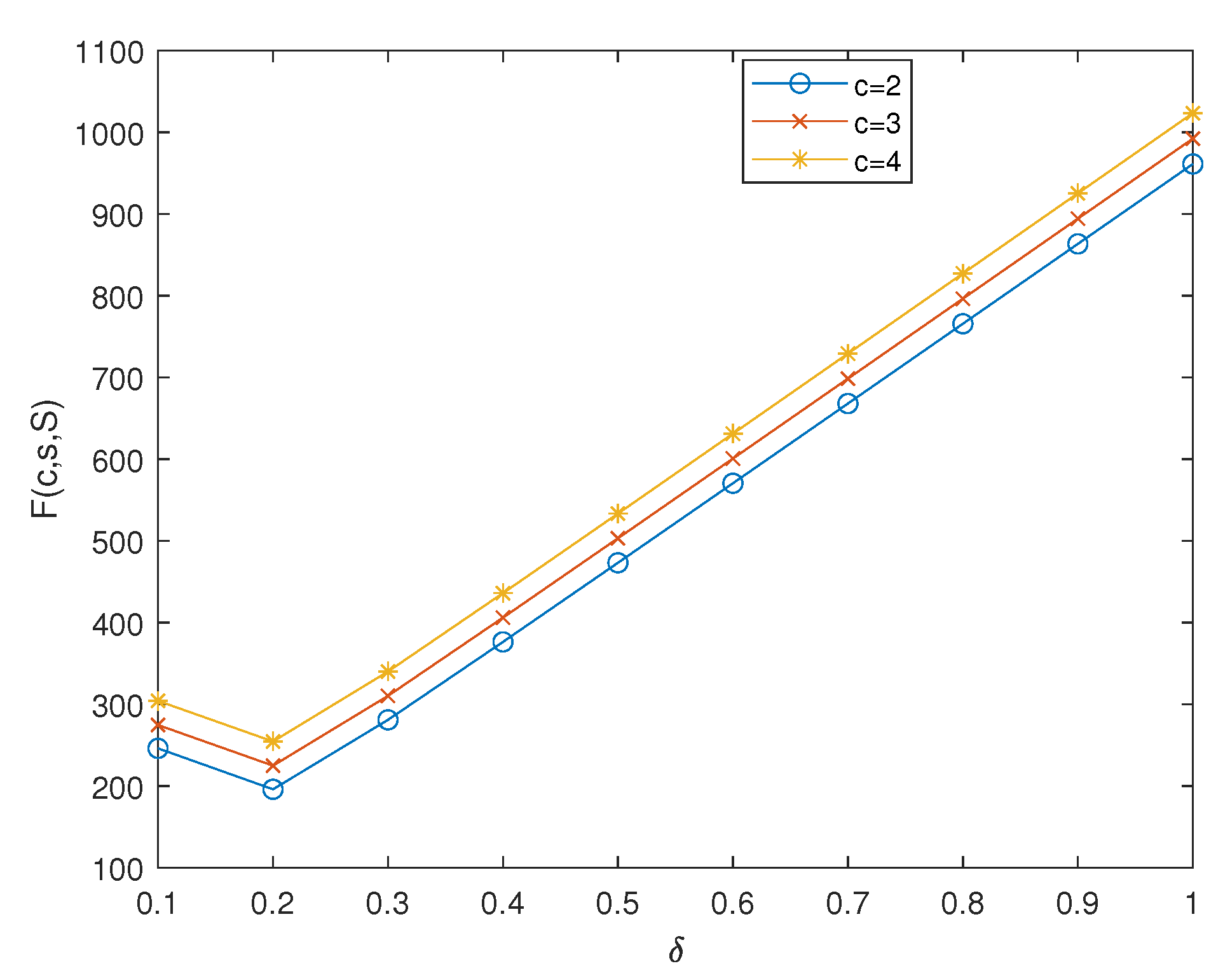
Table 10.
Effect of on .
Table 10.
Effect of on .
| 0.1 | 0.2 | 0.3 | 0.4 | 0.5 | 0.6 | 0.7 | 0.8 | 0.9 | 1 |
|---|
| 246.0757 | 195.9772 | 280.9794 | 376.3558 | 473.1766 | 570.4884 | 668.0241 | 765.6783 | 863.4014 | 961.1673 |
| 274.6499 | 224.8902 | 310.326 | 406.0481 | 503.1662 | 600.737 | 698.5022 | 796.3634 | 894.2765 | 992.2195 |
| 304.1992 | 254.5151 | 340.1136 | 436.0469 | 533.3815 | 631.1632 | 729.1311 | 827.1869 | 925.2874 | 1023.4 |
Table 11.
Optimal server and corresponding minimum cost for .
Table 11.
Optimal server and corresponding minimum cost for .
| 0.1 | 0.2 | 0.3 | 0.4 | 0.5 | 0.6 | 0.7 | 0.8 | 0.9 | 1 |
|---|
| 2 | 3 | 4 | 4 | 5 | 5 | 5 | 5 | 5 | 5 |
| 445.5808 | 477.6176 | 419.2914 | 349.7553 | 318.587 | 318.0415 | 322.3932 | 326.9127 | 330.8801 | 334.2469 |


