Experimental Study of Excessive Local Refinement Reduction Techniques for Global Optimization DIRECT-Type Algorithms

Abstract

This article considers a box-constrained global optimization problem for Lipschitz continuous functions with an unknown Lipschitz constant. The well-known derivative-free global search algorithm DIRECT (DIvide RECTangle) is a promising approach for such problems. Several studies have shown that recent two-step (global and local) Pareto selection-based algorithms are very efficient among all DIRECT-type approaches. However, despite its encouraging performance, it was also observed that the candidate selection procedure has two possible shortcomings. First, there is no limit on how small the size of selected candidates can be. Secondly, a balancing strategy between global and local candidate selection is missing. Therefore, it may waste function evaluations by over-exploring the current local minimum and delaying finding the global one. This paper reviews and employs different strategies in a two-step Pareto selection framework (1-DTC-GL) to overcome these limitations. A detailed experimental study has revealed that existing strategies do not always improve and sometimes even worsen results. Since 1-DTC-GL is a DIRECT-type algorithm, the results of this paper provide general guidance for all DIRECT-type algorithms on how to deal with excessive local refinement more efficiently.

1. Introduction

In this paper, we consider a box-constrained global optimization problem of the form:

$$\begin{array}{cccc}\hfill & \underset{\mathbf{x}\in D}{min}\hfill & \hfill & f\left(\mathbf{x}\right),\hfill \end{array}$$

(1)

where $f:{\mathbb{R}}^n\to \mathbb{R}$ suppose to be the Lipschitz-continuous objective function, $\mathbf{x}$ is the input vector, and the feasible region $\left(D\right)$ is an n-dimensional hyper-rectangle $D=[\mathbf{a},\mathbf{b}]=\{\mathbf{x}\in {\mathbb{R}}^n:a_j\le x_j\le b_j,j=1,\cdots ,n\}$. The objective function can be non-linear, non-differentiable, non-convex, multi-modal, and potentially a “black-box.” In a black-box case, analytical information is unavailable and can be obtained only by evaluating the function at feasible points. Therefore, traditional derivative-information based local optimization methods cannot be used in this situation.

Among derivative-free global optimization algorithms addressing the black-box problem, two main classes [1] are stochastic meta-heuristic algorithms [2,3,4] and deterministic ones [5,6]. The DIRECT algorithm developed by Jones [7] is a popular and widely used deterministic solution technique for various real-world optimization problems [8,9,10,11,12]. The proposed algorithm is an extension of the classical Lipschitz optimization [13,14,15], which no longer requires the knowledge of the Lipschitz constant. The DIRECT algorithm [7] seeks global optima by dividing the most promising hyper-rectangles and evaluating the objective function at their centers.

Since the original algorithm introduction, many researchers have suggested various modifications or extensions of the DIRECT algorithm in various directions. Recent extensive numerical studies [1,16,17] show that DIRECT-type algorithms are often among the most efficient derivative-free global optimization solution techniques. Various hybridized approaches [10,18,19] that are enriched with local search procedures are among the most effective [16,17,20]. However, on average, among traditional (non-hybridized) DIRECT-type algorithms, two-step (global and local) Pareto selection scheme-based approaches, DIRECT-GL [17], 1-DTC-GL [21], often showed the best performance [17]. Moreover, for complex multi-modal and non-convex problems, they often outperformed hybrid ones.

Nevertheless, in a recent survey [22], two possible shortcomings of such two-step Pareto selection were specified. First, these scheme-based algorithms have no protection against “over-exploring” a local minimum, e.g., no limitation of how small the size of selected potentially optimal hyper-rectangles (POHs) can be. Secondly, a balancing strategy between global and local candidate selection is missing. The two-step-based Pareto selection scheme performs global and local search-oriented selection at each iteration. If the current best solution has remained unchanged for several iterations, it can be deduced that the local selection step is potentially unnecessary.

We note that some proposals and studies have already been carried out in the context of the DIRECT algorithm. In [17], we have experimentally investigated a few strategies [7,23,24,25,26] devoted to preventing the original DIRECT algorithm from selecting tiny hyper-rectangles around current local minima. Moreover, the same study also investigated different strategies for balancing global and local phases [10,18,27,28]. However, we cannot generalize from these results which strategy is the most efficient, as individual algorithms were compared, which may have varied not only in the selection step but also in other steps such as partitioning and sampling. It is therefore unclear which of the proposed improvements has the most potential to prevent excessive local refinement.

Contributions and Structure

The main contributions of this work are summarized below:

• It reviews the proposed techniques for excessive local refinement reduction for DIRECT-type algorithms.
• It experimentally validates them on one of the fastest two-step Pareto selection based 1-DTC-GL algorithm.
• It accurately assesses the impact of each of them and, based on these results, makes recommendations for DIRECT-type algorithms in general.
• All six of the newly developed DIRECT-type algorithmic variations are freely available to anyone, ensuring complete reproducibility and re-usability of all results.

The rest of the paper is organized as follows. Section 2.1 reviews the original DIRECT algorithm. Section 2.2 describes a two-step Pareto selection-based DIRECT-GL algorithm. The review of existing local refinement reduction techniques for DIRECT-type algorithms is given in Section 2.3. New 1-DTC-GL algorithmic variations are given in Section 2.4. The numerical investigation using 287 DIRECTGOLib v1.2 test problems is presented and discussed in Section 3. Finally, Section 4 concludes the paper and highlights possible future directions.

2. Materials and Methods

This section introduces the original DIRECT and 1-DTC-GL algorithms. Additionally, existing strategies for preventing excessive refinement around the current minima are reviewed, summarizing their strengths and weaknesses.

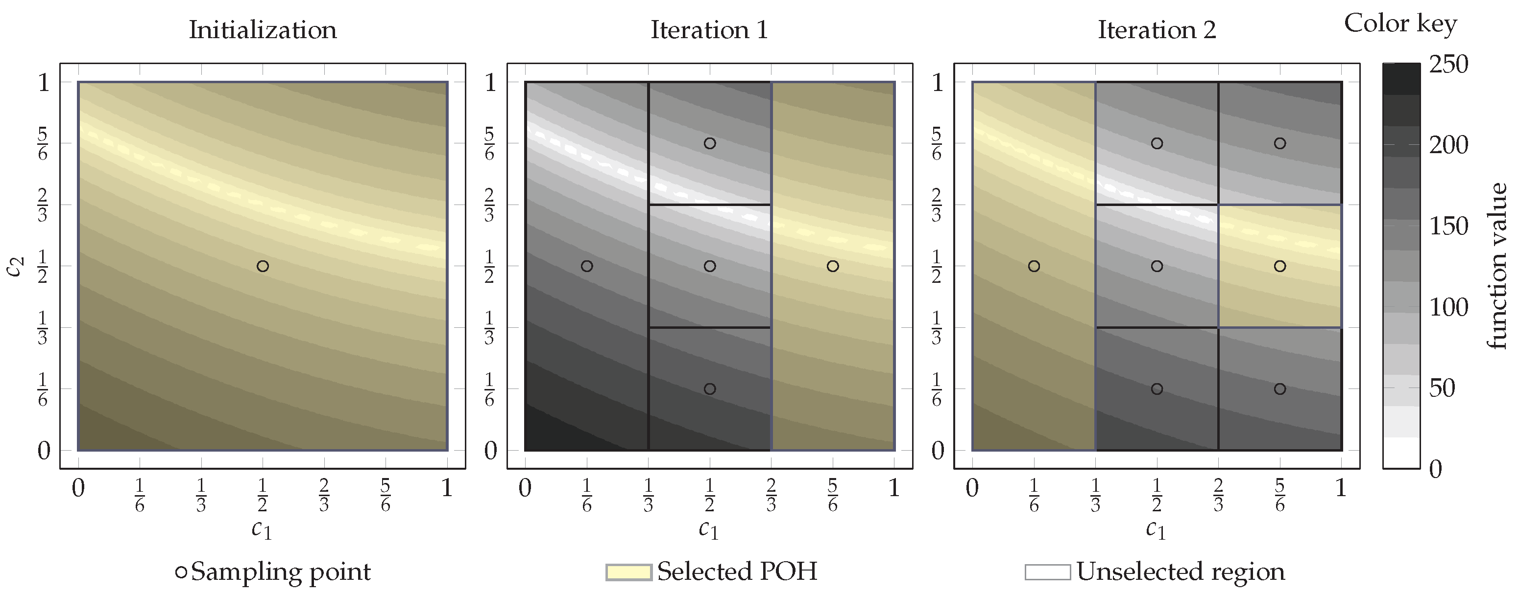
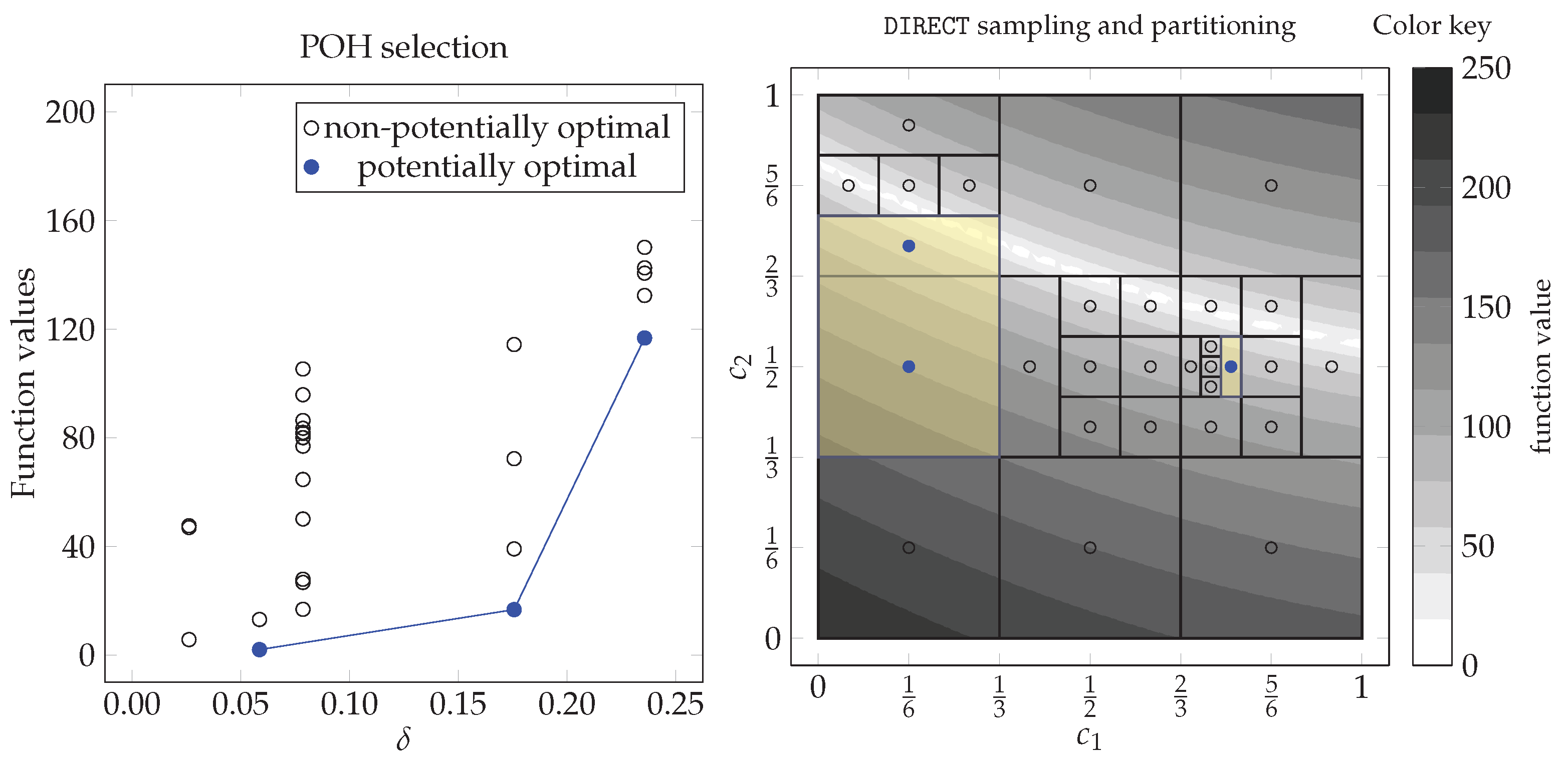
2.1. Overview of the DIRECT Algorithm

The original DIRECT algorithm applies to box-constrained problems and works most of the time in the normalized domain. Therefore, the DIRECT algorithm initially normalizes the domain $D=[\mathbf{a},\mathbf{b}]$ to the unit hyper-rectangle $\overline{D}=[\mathbf{0},\mathbf{1}]=\{\mathbf{x}\in {\mathbb{R}}^n:0\le a_j\le x_j\le b_j\le 1,j=1,\cdots ,n\}$. The algorithm only refers to the original space $\left(D\right)$ when performing objective function evaluations. Therefore, when we say that the value of the objective function is evaluated at $f\left(\mathbf{c}\right)$, where $\mathbf{c}\in \overline{D}$ is the midpoint of the hyper-rectangle, it means that the corresponding midpoint of the original domain ($\mathbf{x}\in D$) is used, i.e.,

$$f\left(\mathbf{c}\right)=f\left(\mathbf{x}\right),\mathrm{where}{x}_j=(b_j-a_j)c_j+a_j,j=1,\cdots ,n.$$

(2)

The DIRECT algorithm starts the search by evaluating the objective function at the midpoint ${\mathbf{c}}^1=(1/2,\cdots ,1/2)$ of the initial unit hyper-rectangle $\overline{D}={\overline{D}}_0^1$. Then, the algorithm identifies and selects potentially optimal hyper-rectangles. Initially, only one hyper-rectangle is available (see the left panel in Figure 1). Therefore, selection is trivial. After this, DIRECT creates new midpoints at the positions

$${\mathbf{c}}^1\pm \frac{1}{3}{d}^m{\mathbf{e}}_j,j\in M,$$

(3)

where $d^m$ is the maximum side length, M is a set of coordinates with the maximum side length, and ${\mathbf{e}}_j$ is the jth unit vector. The DIRECT algorithm uses n-dimensional trisection, so the objective function is evaluated at each POH only once. The midpoint of selected POH becomes the midpoint of the new smaller “middle” third hyper-rectangle and does not requires additional re-evaluation.

If POH has more than one longest coordinate, i.e., $card\left(M\right)>1$ (e.g., for the n-dimensional initial hyper-rectangle $card\left(M\right)=n$), DIRECT starts trisection from the coordinate ($j\in M$) with the lowest $w_j$ value

$$w_j=min\{f({\mathbf{c}}^1+\frac{1}{3}{d}^m{\mathbf{e}}_j),f({\mathbf{c}}^1-\frac{1}{3}{d}^m{\mathbf{e}}_j)\},j\in M,$$

(4)

and continues to the highest [7,22]. By using this procedure, it is ensured that lower function values are placed in larger hyper-rectangles. It can be seen in the middle panel of Figure 1. If all coordinates are equal, $2n+1$ new smaller non-overlapping hyper-rectangles of n distinct measures are created. Figure 1 demonstrates the selection, sampling, and partitioning process at the initialization and the first two DIRECT iterations on the two-dimensional Bukin6 test problem.

In contrast to initialization, from the first iteration onward ($k>1$), the selection of the so-called “potentially optimal” hyper-rectangles that should be further explored is not trivial. Let us formalize this selection process.

Let the current partition in iteration k be defined as

$${\mathcal{P}}_k=\{{\overline{D}}_k^i:i\in {\mathbb{I}}_k\},$$

where ${\overline{D}}_k^i=[{\mathbf{a}}_k^i,{\mathbf{b}}_k^i]=\{\mathbf{x}\in \overline{D}:0\le a_{k_j}^i\le x_j\le b_{k_j}^i\le 1,j=1,\cdots ,n,\forall i\in {\mathbb{I}}_k\}$ and ${\mathbb{I}}_k$ is the index set identifying the current partition ${\mathcal{P}}_k$. The next partition, ${\mathcal{P}}_{k+1}$, is obtained by subdividing selected POHs from the current partition ${\mathcal{P}}_k$. Note that at the first iteration, there is only one candidate, ${\overline{D}}_1^1$, which is automatically potentially optimal. The formal requirement of potential optimality in future iterations is stated in Definition 1.

Definition 1.

Let ${\mathbf{c}}^i$ denote the center sampling point and ${\delta }_k^i$ be a measure (equivalently, sometimes called distance or size) of the hyper-rectangle ${\overline{D}}_k^i$. Let $\epsilon >0$ be a positive constant and $f^{min}$ be the best currently found value of the objective function. A hyper-rectangle ${\overline{D}}_k^h,h\in {\mathbb{I}}_k$ is said to be potentially optimal if there exists some rate-of-change (Lipschitz) constant $\tilde{L}>0$ such that

$$\begin{array}{ccc}\hfill f\left({\mathbf{c}}^h\right)-\tilde{L}{\delta }_k^h& \le & f\left({\mathbf{c}}^i\right)-\tilde{L}{\delta }_k^i,\forall i\in {\mathbb{I}}_k,\hfill \end{array}$$

(5)

$$\begin{array}{ccc}\hfill f\left({\mathbf{c}}^h\right)-\tilde{L}{\delta }_k^h& \le & f^{min}-\epsilon \left|f^{min}\right|,\hfill \end{array}$$

(6)

where the measure of the hyper-rectangle ${\overline{D}}_k^i$ is

$${\delta }_k^i=\frac{1}{2}\parallel {\mathbf{b}}^i-{\mathbf{a}}^i\parallel .$$

(7)

The hyper-rectangle ${\overline{D}}_k^h$ is potentially optimal if the lower Lipschitz bound for the objective function computed by the left-hand side of (5) is the smallest one with some positive constant $\tilde{L}$ in the current partition ${\mathcal{P}}_k$. A geometrical interpretation of POH selection using Definition 1 is illustrated on the left side of Figure 2. Here, each hyper-rectangle is represented as a point whose horizontal coordinate is equal to the measure (${\delta }_k^i$) and vertical coordinate is equal to the function value attained at the midpoint $\left({\mathbf{c}}^{\mathbf{i}}\right)$. The hyper-rectangles satisfying Definition 1 are marked in blue and correspond to the lower-right convex hull of the points. Selected hyper-rectangles are then sampled and subdivided. This process continues until some stopping condition is satisfied and is summarized in Algorithm 1.

Algorithm 1: Main steps of the DIRECT algorithm

2.2. Two-Step Pareto Selection Based 1-DTC-GL Algorithm

Our previous work [29] introduced a new two-step Pareto selection [30] based algorithm DIRECT-GL. In [21], we investigated the most efficient partitioning schemes combined with a Pareto selection based on two steps. Hyper-rectangular partitioning based on 1-Dimensional Trisection and sampling at the Center points combined with two-step (Global and Local) Pareto selection (1-DTC-GL) was one of the most efficient DIRECT-type approaches. The POH selection in 1-DTC-GL is the most significant difference compared to the original DIRECT. In each iteration, 1-DTC-GL performs the identification of POHs twice. Both times, it selects only Pareto-optimal hyper-rectangles. In the following, we formally state two algorithms used to find them.

Let ${\mathbb{L}}_k$ be the set of all different indices at the current partition ${\mathcal{P}}_k$, corresponding to the groups of hyper-rectangles having the same measure ${\delta }_k$. Then, the minimum value $l_k^{\min }\in {\mathbb{L}}_k$ corresponds to the group of hyper-rectangles having the smallest measure ${\delta }_k^{\min }$, while $l_k^{\max }\in {\mathbb{L}}_k$—having the largest measure ${\delta }_k^{\max }$, i. e., $l_k^{\max }=max\left\{{\mathbb{L}}_k\right\}<\infty$. Algorithm 2 presents the main steps for identifying Pareto optimal hyper-rectangles, i.e., non-dominated on measure (the higher, the better) and midpoint function value (the lower, the better).

Algorithm 2: Pareto selection enhancing the global search

Similarly, Algorithm 3 selects the hyper-rectangles that are non-dominated in measure and distance from the current minimum point (the closer, the better). When both steps are completed, the unique union of these two sets, $S_k^{\mathrm{G}}$ from Algorithm 2 and $S_k^{\mathrm{L}}$ from Algorithm 3, is used. This way, in 1-DTC-GL, the set of POHs is enlarged with various size hyper-rectangles nearest the current minimum point $\left({\mathbf{c}}^{\min }\right)$, ensuring a broader examination around the current minima.

Algorithm 3: Pareto selection enhancing the local search

input: Current partition ${\mathcal{P}}_k$ and related information; output: Set of selected POHs $\left(S_k^{\mathrm{LS}}\right)$;

Set $S_k^{\mathrm{L}}=\varnothing$; At each iteration k, evaluate the Euclidean distance from the current minimum point $\left({\mathbf{c}}^{\min }\right)$ to other sampled points: $$d({\mathbf{c}}^{\min },{\mathbf{c}}^i)=\sqrt{\sum _{j=1}^n{(c_j^{\min }-c_j^i)}^2}$$ (9) Apply Algorithm 2 using $d({\mathbf{c}}^{\min },{\mathbf{c}}^i)$ instead of $f\left({\mathbf{x}}^i\right)$ in (8); Return$S_k^{\mathrm{LS}}$;

Let us summarize the differences between the two-step Pareto selection schemes and the original DIRECT. The selection of POH in 1-DTC-GL is performed twice, taking into account the objective function values and Euclidean distances from the current minima. This way, the set of POHs is enlarged by considering more medium-sized hyper-rectangles and may be more global. The local selection step includes more hyper-rectangles around current minima. In this way, refinement of the solution is accelerated. On the other hand, it can have the opposite effect, as this selection scheme does not protect against over-exploration in sub-optimal regions. In the original DIRECT, the parameter $\epsilon$ in Equation (6) is used to protect against this [7,28]. However, in 1-DTC-GL, even a tiny hyper-rectangle, where only negligible improvement can be expected, can be selected. Furthermore, the local selection step may be excessive when the current minima $\left(f^{\min }\right)$ do not improve in a series of consecutive iterations.

2.3. Review of Excessive Local Refinement Reduction Techniques

This section reviews techniques introduced in the DIRECT literature for reducing excessive local refinement.

2.3.1. Replacing the Minimum Value with an Average and Median Values

In the original selection of POHs, Equation (6) in Definition 1 is used to protect against excessive refinement around the current local minima [7,28]. In [7], the authors obtained good results for values of $\epsilon$ ranging from ${10}^{-3}$ to ${10}^{-7}$, while in [24,26,31,32], the authors introduced an adaptive scheme for the parameter $\epsilon$.

However, in [23], it was observed that such a selection strategy is sensitive to additive scaling of the objective function. Additionally, the DIRECT algorithm performs poorly when the objective function values are large. To overcome this, the authors suggested scaling the values of the functions by subtracting the median value $(f^{\mathrm{median}}$) calculated from all the collected values. Formally, a new DIRECT variation, called DIRECT-m, replaces Equation (6) with:

$$f\left({\mathbf{x}}^h\right)-\tilde{L}{\delta }_k^h\le f^{\min }-\epsilon |f^{\min }-f^{\mathrm{median}}|.$$

(10)

A few years later, a similar idea was extended in [25]. Again, to reduce the sensitivity for additive scaling of the objective function, the authors of the DIRECT-a algorithm proposed using the average value $\left(f^{\mathrm{average}}\right)$ instead:

$$f\left({\mathbf{x}}^h\right)-\tilde{L}{\delta }_k^h\le f^{\min }-\epsilon |f^{\min }-f^{\mathrm{average}}|.$$

(11)

Equations (10) and (11) also work also work as protection from over-exploration of the local minima.

2.3.2. Limiting the Measure of Hyper-Rectangles

In [33], the authors introduced the aggressive selection of POH. This strategy selects at least one hyper-rectangle from each group of different measures $\left({\delta }_k^i\right)$ with the lowest function value. This way, the set of POHs enlarges by including non-potentially Lipschitz optimal hyper-rectangles. Although this solution positively affected parallelism [34], it did not have a strong positive effect on sequential algorithms of type DIRECT. In the sequential context, the apparent shortcoming is that hyper-rectangles proliferate as the number of iterations increases, often leading to a memory allocation failure.

To overcome it, the authors in [34] suggested limiting the refinement of the search space when the measure of hyper-rectangles $\left({\delta }_k^i\right)$ reached some prescribed limit $\left({\delta }^{\mathrm{limit}}\right)$. It has been shown that memory usage may be reduced from $10\%$ to $70\%$. The parameter ${\delta }^{\mathrm{limit}}$ has the same purpose as Equation (6), i.e., to avoid wasting function evaluations by “over-exploring” the local minimum. The authors of [21] have set ${\delta }^{\mathrm{limit}}$ to the size of a hyper-rectangle subdivided $50n$ times. It is a relatively small and safe value since the choice of the parameter ${\delta }^{\mathrm{limit}}$ can be dangerous. More significant value can prevent the algorithm from reaching the minimum within the required tolerance.

2.3.3. Balancing the Local and Global Searches

Jones in [22] argued the need for the strategy to better balance emphasis on the local and global search. An approach could be to run a local search subroutine when there is an improvement in the current minima value [18]. However, this would already be a hybridized DIRECT-type algorithm requiring incorporating a separate local algorithm. This paper focuses on strategies without leaving the DIRECT algorithm framework.

Another approach for balancing the emphasis on the global and local search within the DIRECT-type method is the two-phase “globally-biased” technique. DIRECT-type globally-biased algorithms were proposed and experimentally investigated recently [10,28]. The suggested algorithms operate in the traditional phase until a sufficient number of subdivisions have been completed without improving $f^{\min }$. Once $f^{\min }$ is explored well, the algorithm switches to the global phase and examines larger and far away hyper-rectangles. The algorithm switches back to the traditional phase when the $f^{\min }$ value is improved. It also performs one “security” iteration of the traditional phase at every certain number of iterations. Therefore, the global phase reduces the number of POHs, excluding small hyper-rectangles around the well-explored minimum.

2.4. New Two-Step Pareto Selection Based Algorithmic Variations for Excessive Local Refinement Reduction

In this section, we define six novel 1-DTC-GL algorithmic variations to reduce the potentially excessive local refinement of the original two-step Pareto selection scheme.

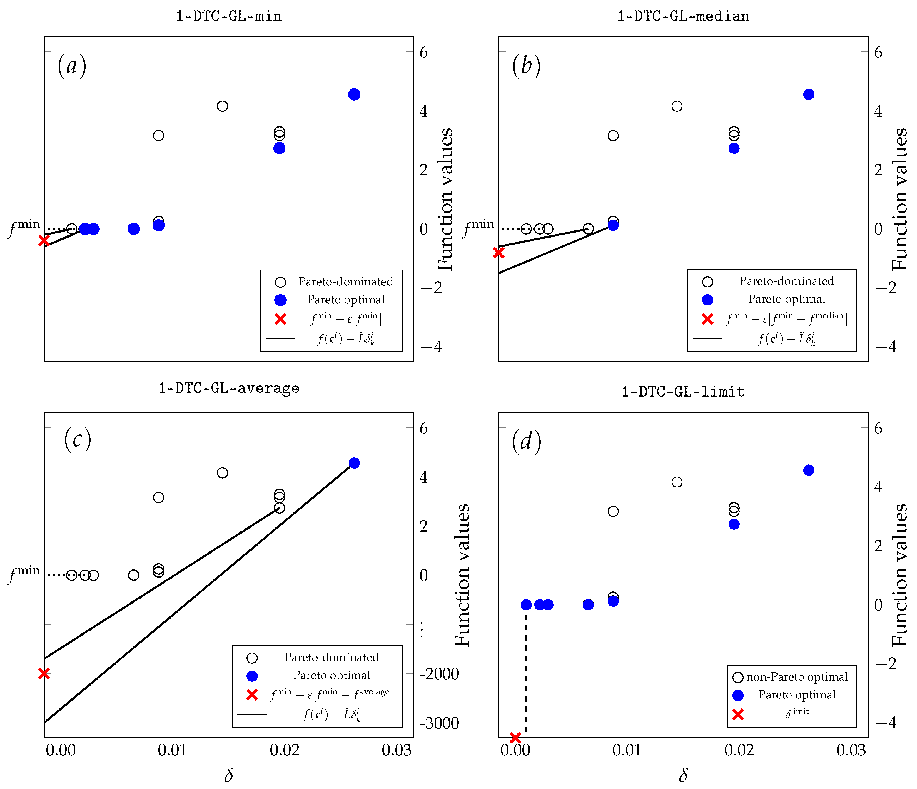
2.4.1. 1-DTC-GL-min Algorithm

The 1-DTC-GL-min algorithm incorporates Equation (6) from Definition 1 into the original two-step Pareto selection scheme. Therefore, in Algorithm 2, Line 2, $l_k^{\min }$ is set to the group of hyper-rectangles with the lowest ${\delta }_k^{\min }$ such that Equation (6) still holds. When such a candidate is found, a traditional two-step Pareto selection scheme is applied between hyper-rectangles of larger diameters.

The candidate selection of 1-DTC-GL-min is illustrated in part $\left(a\right)$ of Figure 3. The illustrative example is given on a two-dimensional Csendes test problem in the thirteenth iteration of the algorithm. Since the considered techniques do not affect the selection of larger hyper-rectangles, the x-axis is limited to $0.03$. The y-axis has also been reduced to demonstrate the effectiveness of the strategies under consideration.

Here, the current minimum value is very close to zero $(f^{\min }\approx {10}^{-12})$. Equation (6) requires the Lipschitz lower bound to be less than $f^{\min }-\epsilon \left|f^{\min }\right|$. Therefore, 1-DTC-GL-min excludes tiny hyper-rectangles where the value of the objective function at their midpoint is close to the $f^{\min }$ value. When the current best point is not the global one, selecting tiny hyper-rectangles could significantly delay the discovery of the global one.

2.4.2. 1-DTC-GL-median Algorithm

The 1-DTC-GL-median algorithm incorporates Equation (10) into the original two-step Pareto selection scheme. In 2 2, 1-DTC-GL-median sets $l_k^{\min }$ to the group of hyper-rectangles with the lowest measure $\left({\delta }_k^{\min }\right)$ such that Equation (10) still holds. As for 1-DTC-GL-min, when such a hyper-rectangle is found, a traditional two-step Pareto selection scheme is applied between hyper-rectangles of larger diameters.

The result of 1-DTC-GL-median selection is illustrated in part $\left(b\right)$ of Figure 3. Equation (10) requires the Lipschitz lower bound to be less than $f^{\min }-\epsilon |f^{\min }-f^{\mathrm{median}}|$. Since the median value is much higher than 0, 1-DTC-GL-median selects less small hyper-rectangles than 1-DTC-GL-min. This makes the search more global, but can also have a negative impact on the refinement of the global solution.

2.4.3. 1-DTC-GL-average Algorithm

The 1-DTC-GL-average algorithm incorporates Equation (11) into the original two-step Pareto selection scheme. In Algorithm 2, Line 2, 1-DTC-GL-average sets $l_k^{\min }$ to the group of hyper-rectangles with the slightest measure $\left({\delta }_k^{\min }\right)$ such that Equation (11) still holds. The selection between larger hyper-rectangles is analogous to the 1-DTC-GL-min and 1-DTC-GL-median algorithms.

The result of 1-DTC-GL-average selection is illustrated in part $\left(c\right)$ of Figure 3. Equation (11) requires the Lipschitz lower bound to be less than $f^{\min }-\epsilon |f^{\min }-f^{\mathrm{average}}|$. Since the Csende test problem has large extreme values, $f^{\mathrm{average}}$ is much larger than $f^{\mathrm{median}}$. Thus, the 1-DTC-GL-average makes the search even more global 1-DTC-GL-median, which can hurt the refinement of the global solution, requiring the selection of smaller hyper-rectangles.

2.4.4. 1-DTC-GL-limit Algorithm

1-DTC-GL-limit limits the refinement of the search space when the measure of hyper-rectangles reaches some prescribed limit ${\delta }^{\mathrm{limit}}$. In 1-DTC-GL-limit, ${\delta }^{\mathrm{limit}}$ is set to the size of a hyper-rectangle subdivided $20n$ times. Furthermore, regardless of the hyper-rectangle measure, 1-DTC-GL-limit always selects the hyper-rectangle with $f^{\min }$.

The result of 1-DTC-GL-limit selection is illustrated in part $\left(d\right)$ of Figure 3. Since all hyper-rectangles have measures ${\delta }_{13}^i\ge {\delta }^{\mathrm{limit}},\forall i$, the selected set is the same as for the 1-DTC-GL. The differences will appear in later iterations when the hyper-rectangles already subdivided more than 20 times appear.

2.4.5. 1-DTC-GL-gb Algorithm

1-DTC-GL-gb incorporates the “globally-biased” technique into a two-step Pareto selection scheme. The 1-DTC-GL-gb algorithm performs traditional two-step Pareto selection, using Algorithms 2 and 3, until a sufficient number of subdivisions have been completed without improving $f^{\min }$. Once $f^{\min }$ has been well explored, the 1-DTC-GL-gb algorithm switches to the global phase and performs only Pareto selection improving the global search (Algorithm 2). The 1-DTC-GL-gb algorithm switches back to the traditional phase when the $f^{\min }$ value is improved and during “security” iteration. Finally, we note that the recommended values [10,28] for the additional parameters necessary to switch between phases are used in 1-DTC-GL-gb.

2.4.6. 1-DTC-GL-rev Algorithm

1-DTC-GL-rev incorporates the idea from [18], i.e., it performs the local search selection using Algorithm 3 only when there is an improvement in $f^{\min }$. The rest of the time, it selects hyper-rectangles using only Algorithm 2 and reduces the impact on local search.

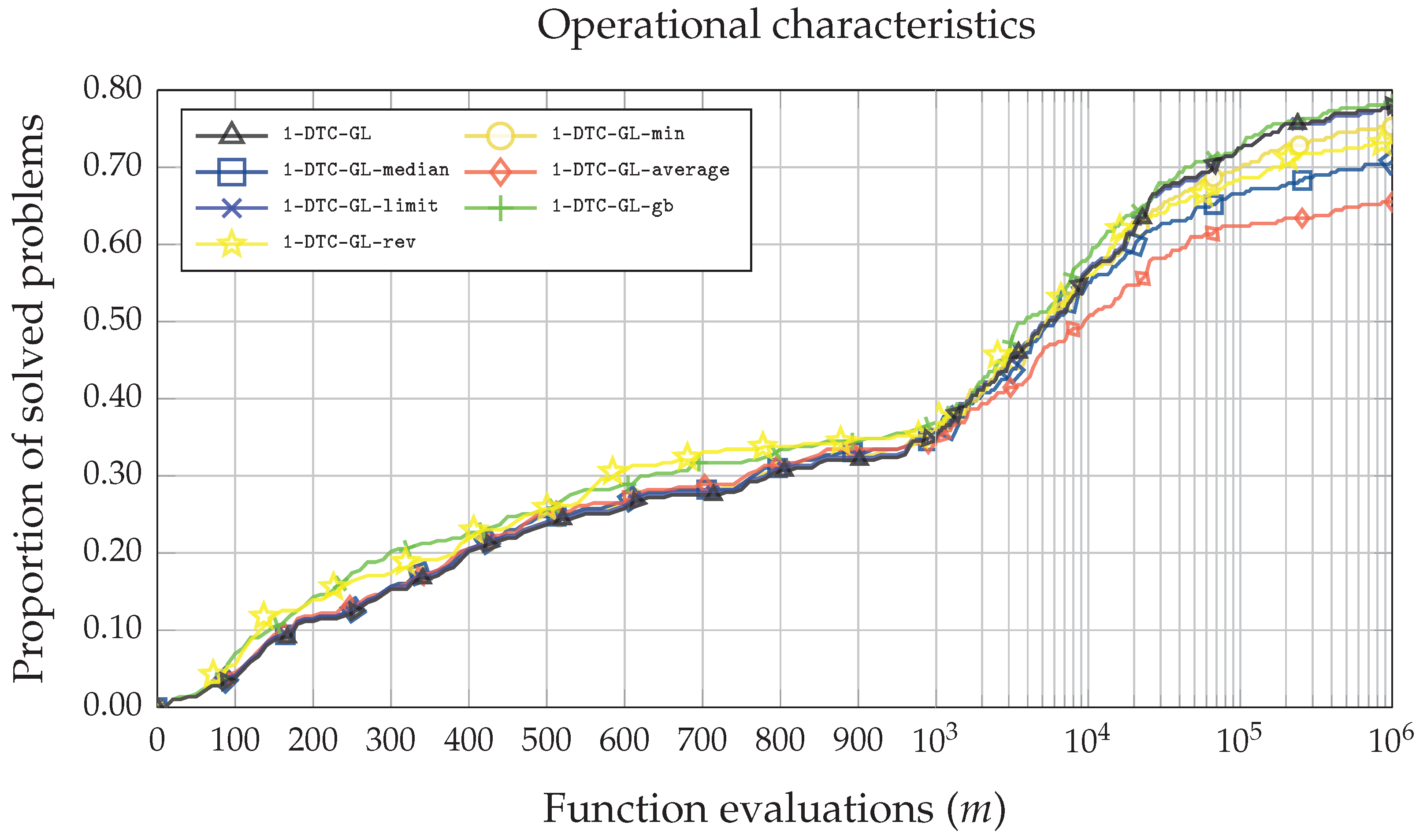
3. Results and Discussions

In this section, we compare the performance of six techniques for reducing the local refinement applied to the 1-DTC-GL algorithm, which showed promising results in our recent computational studies [17,21]. Six newly constructed algorithmic modifications are empirically evaluated and compared with the original 1-DTC-GL algorithm. The algorithmic variations are examined using the most up-to-date version of the DIRECTGOLib v1.2 [35] library. A summary and properties of all box-constrained optimization problems from DIRECTGOLib v1.2 [35] are given in Appendix A,

Table A1. Key characteristics of box-constrained global optimization problems with fixed n from DIRECTGOLib v1.2 [35]. Data adapted from [20].

#	Name	Source	n	D	$\tilde{\mathit{D}}$	Type	No. of Minima	${\mathit{f}}^{*}$
1	AckleyN2${}^{\alpha }$	[40]	2	${[-15,30]}^n$	${[-18,47]}^n$	uni-modal	convex	$-200.0000$
2	AckleyN3${}^{\alpha }$	[40]	2	${[-15,30]}^n$	${[-18,47]}^n$	uni-modal	convex	$-186.4112$
3	AckleyN4${}^{\alpha }$	[40]	2	${[-15,30]}^n$	${[-18,47]}^n$	non-convex	multi-modal	$-4.5901$
4	Adjiman	[40]	2	${[-1,2]}^n$	-	non-convex	multi-modal	$-2.0218$
5	BartelsConn${}^{\alpha }$	[40]	2	${[-500,500]}^n$	${[-300,700]}^n$	non-convex	multi-modal	$1.0000$
6	Beale	[41,42]	2	${[-4.5,4.5]}^n$	-	non-convex	multi-modal	$0.0000$
7	BiggsEXP2	[40]	2	${[0,20]}^n$	-	non-convex	multi-modal	$0.0000$
8	BiggsEXP3	[40]	3	${[0,20]}^n$	-	non-convex	multi-modal	$0.0000$
9	BiggsEXP4	[40]	4	${[0,20]}^n$	-	non-convex	multi-modal	$0.0000$
10	BiggsEXP5	[40]	5	${[0,20]}^n$	-	non-convex	multi-modal	$0.0000$
11	BiggsEXP6	[40]	6	${[0,20]}^n$	-	non-convex	multi-modal	$0.0000$
12	Bird	[40]	2	${[-2\pi ,2\pi ]}^n$	-	non-convex	multi-modal	$-106.7645$
13	Bohachevsky1${}^{\alpha }$	[41,42]	2	${[-100,100]}^n$	${[-55,145]}^n$	convex	uni-modal	$0.0000$
14	Bohachevsky2${}^{\alpha }$	[41,42]	2	${[-100,100]}^n$	${[-55,145]}^n$	non-convex	multi-modal	$0.0000$
15	Bohachevsky3${}^{\alpha }$	[41,42]	2	${[-100,100]}^n$	${[-55,145]}^n$	non-convex	multi-modal	$0.0000$
16	Booth	[41,42]	2	${[-10,10]}^n$	-	convex	uni-modal	$0.0000$
17	Brad	[40]	3	$[-0.25,0.25]\times {[0.01,2.5]}^2$	-	non-convex	multi-modal	$6.9352$
18	Branin	[41,43]	2	$[-5,10]\times [10,15]$	-	non-convex	multi-modal	$0.3978$
19	Bukin4	[40]	2	$[-15,-5]\times [-3,3]$	-	convex	multi-modal	$0.0000$
20	Bukin6	[42]	2	$[-15,5]\times [-3,3]$	-	convex	multi-modal	$0.0000$
21	CarromTable	[44]	2	${[-10,10]}^n$	-	non-convex	multi-modal	$-24.1568$
22	ChenBird	[40]	2	${[-500,500]}^n$	-	non-convex	multi-modal	$-2000.0000$
23	ChenV	[40]	2	${[-500,500]}^n$	-	non-convex	multi-modal	$-2000.0009$
24	Chichinadze	[40]	2	${[-30,30]}^n$	-	non-convex	multi-modal	$-42.9443$
25	Cola	[40]	17	${[-4,4]}^n$	-	non-convex	multi-modal	$12.0150$
26	Colville	[41,42]	4	${[-10,10]}^n$	-	non-convex	multi-modal	$0.0000$
27	Cross_function	[44]	2	${[-10,10]}^n$	-	non-convex	multi-modal	$0.00004$
28	Cross_in_Tray	[42]	2	${[0,10]}^n$	-	non-convex	multi-modal	$-2.0626$
29	CrownedCross	[44]	2	${[-10,15]}^n$	-	non-convex	multi-modal	$0.0001$
30	Crosslegtable	[44]	2	${[-10,15]}^n$	-	non-convex	multi-modal	$-1.0000$
31	Cube	[44]	2	${[-10,10]}^n$	-	convex	multi-modal	$0.0000$
32	Damavandi	[44]	2	${[0,14]}^n$	-	non-convex	multi-modal	$0.0000$
33	Dejong5	[42]	2	${[-65.536,65.536]}^n$	-	non-convex	multi-modal	$0.9980$
34	Dolan	[40]	5	${[-100,100]}^n$	-	non-convex	multi-modal	$-529.8714$
35	Drop_wave${}^{\alpha }$	[42]	2	${[-5.12,5.12]}^n$	${[-4,6]}^n$	non-convex	multi-modal	$-1.0000$
36	Easom${}^{\alpha }$	[41,42]	2	${[-100,100]}^n$	${[-100{(i+1)}^{-1},100i]}^i$	non-convex	multi-modal	$-1.0000$
37	Eggholder	[42]	2	${[-512,512]}^n$	-	non-convex	multi-modal	$-959.6406$
38	Giunta	[44]	2	${[-1,1]}^n$	-	non-convex	multi-modal	$0.0644$
39	Goldstein_and _Price${}^{\alpha }$	[41,43]	2	${[-2,2]}^n$	${[-1.1,2.9]}^n$	non-convex	multi-modal	$3.0000$
40	Hartman3	[41,42]	3	${[0,1]}^n$	-	non-convex	multi-modal	$-3.8627$
41	Hartman4	[41,42]	4	${[0,1]}^n$	-	non-convex	multi-modal	$-3.1344$
42	Hartman6	[41,42]	6	${[0,1]}^n$	-	non-convex	multi-modal	$-3.3223$
43	HelicalValley	[44]	3	${[-10,20]}^n$	-	convex	multi-modal	$0.0000$
44	HimmelBlau	[44]	2	${[-5,5]}^n$	-	convex	multi-modal	$0.0000$
45	Holder_Table	[42]	2	${[-10,10]}^n$	-	non-convex	multi-modal	$-19.2085$
46	Hump	[41,42]	2	${[-5,5]}^n$	-	non-convex	multi-modal	$-1.0316$
47	Langermann	[42]	2	${[0,10]}^n$	-	non-convex	multi-modal	$-4.1558$
48	Leon	[44]	2	${[-1.2,1.2]}^n$	-	convex	multi-modal	$0.0000$
49	Levi13	[44]	2	${[-10,10]}^n$	-	non-convex	multi-modal	$0.0000$
50	Matyas${}^{\alpha }$	[41,42]	2	${[-10,10]}^n$	${[-5.5,14.5]}^n$	convex	uni-modal	$0.0000$
51	McCormick	[42]	2	$[-1.5,4]\times [-3,4]$	-	convex	multi-modal	$-1.9132$
52	ModSchaffer1${}^{\alpha }$	[45]	2	${[-100,100]}^n$	${[-100,150]}^n$	non-convex	multi-modal	$0.0000$
53	ModSchaffer2${}^{\alpha }$	[45]	2	${[-100,100]}^n$	${[-100,150]}^n$	non-convex	multi-modal	$0.0000$
54	ModSchaffer3${}^{\alpha }$	[45]	2	${[-100,100]}^n$	${[-100,150]}^n$	non-convex	multi-modal	$0.0015$
55	ModSchaffer4${}^{\alpha }$	[45]	2	${[-100,100]}^n$	${[-100,150]}^n$	non-convex	multi-modal	$0.2925$
56	PenHolder	[41,42]	2	${[-11,11]}^n$	-	non-convex	multi-modal	$-0.9635$
57	Permdb4	[41,42]	4	${[-i,i]}^i$	-	non-convex	multi-modal	$0.0000$
58	Powell	[41,42]	4	${[-4,5]}^n$	-	convex	multi-modal	$0.0000$
59	Power_Sum${}^{\alpha }$	[41,42]	4	${[0,4]}^n$	${[1,4+\sqrt[i]{2}]}^i$	convex	multi-modal	$0.0000$
60	Shekel5	[41,42]	4	${[0,10]}^n$	-	non-convex	multi-modal	$-10.1531$
61	Shekel7	[41,42]	4	${[0,10]}^n$	-	non-convex	multi-modal	$-10.4029$
62	Shekel10	[41,42]	4	${[0,10]}^n$	-	non-convex	multi-modal	$-10.5364$
63	Shubert	[41,42]	2	${[-10,10]}^n$	-	non-convex	multi-modal	$-186.7309$
64	TestTubeHolder	[44]	2	${[-10,10]}^n$	-	non-convex	multi-modal	$-10.8722$
65	Trefethen	[44]	2	${[-2,2]}^n$	-	non-convex	multi-modal	$-3.3068$
66	Wood${}^{\alpha }$	[45]	4	${[-100,100]}^n$	${[-100,150]}^n$	non-convex	multi-modal	$0.0000$
67	Zettl	[44]	2	${[-5,5]}^n$	-	convex	multi-modal	$-0.0037$

i—indexes used for variable bounds (1, …, n). α—domain D was perturbed. The sign “-” means that $\tilde{D}$ is the same as D.

and

Table A2. Key characteristics of box-constrained global optimization problems with varying n from DIRECTGOLib v1.2 [35]. Data adapted from [20].

#	Name	Source	D	$\tilde{\mathit{D}}$	Type	No. of Minima	${\mathit{f}}^{*}$
1	Ackley${}^{\alpha }$	[41,42]	${[-15,30]}^n$	${[-18,47]}^n$	non-convex	multi-modal	$0.0000$
2	AlpineN1${}^{\alpha }$	[44]	${[-10,10]}^n$	${[-10,7.5]}^n$	non-convex	multi-modal	$0.0000$
3	Alpine${}^{\alpha }$	[44]	${[0,10]}^n$	${[\sqrt[i]{2},8+\sqrt[i]{2}]}^i$	non-convex	multi-modal	$-2.{8081}^n$
4	Brown	[40]	${[-1,4]}^n$	-	convex	uni-modal	$0.0000$
5	ChungR	[40]	${[-100,350]}^n$	-	convex	uni-modal	$0.0000$
6	Csendes${}^{\alpha }$	[44]	${[-10,10]}^n$	${[-10,25]}^n$	convex	multi-modal	$0.0000$
7	Cubic	[42]	${[-4,3]}^n$	-	convex	uni-modal	$0.0000$
8	Deb01${}^{\alpha }$	[44]	${[-1,1]}^n$	${[-0.55,1.45]}^n$	non-convex	multi-modal	$-1.0000$
9	Deb02${}^{\alpha }$	[44]	${[0,1]}^n$	${[0.225,1.225]}^n$	non-convex	multi-modal	$-1.0000$
10	Dixon_and_Price	[41,42]	${[-10,10]}^n$	-	convex	multi-modal	$0.0000$
11	Dejong	[42]	${[-3,7]}^n$	-	convex	uni-modal	$0.0000$
12	Exponential	[40]	${[-1,4]}^n$	-	non-convex	multi-modal	$-1.0000$
13	Exponential2	[42]	${[0,7]}^n$	-	non-convex	multi-modal	$0.0000$
14	Exponential3	[42]	${[-30,20]}^n$	-	non-convex	multi-modal	$0.0000$
15	Griewank${}^{\alpha }$	[41,42]	${[-600,600]}^i$	${[-\sqrt{600i},600{\sqrt{i}}^{-1}]}^i$	non-convex	multi-modal	$0.0000$
16	Layeb01${}^{\alpha }$	[46]	${[-100,100]}^n$	${[-100,90]}^n$	convex	uni-modal	$0.0000$
17	Layeb02	[46]	${[-10,10]}^n$	-	convex	uni-modal	$0.0000$
18	Layeb03${}^{\alpha }$	[46]	${[-10,10]}^n$	${[-10,12]}^n$	non-convex	multi-modal	$-n+1$
19	Layeb04	[46]	${[-10,10]}^n$	-	non-convex	multi-modal	$\left(ln\right(0.001)-1)$$(n-1)$
20	Layeb05	[46]	${[-10,10]}^n$	-	non-convex	multi-modal	$\left(ln\right(0.001\left)\right)$$(n-1)$
21	Layeb06	[46]	${[-10,10]}^n$	-	non-convex	multi-modal	$0.0000$
22	Layeb07${}^{\alpha }$	[46]	${[-10,10]}^n$	${[-10,12]}^n$	non-convex	multi-modal	$0.0000$
23	Layeb08	[46]	${[-10,10]}^n$	-	non-convex	multi-modal	$log\left(0.001\right)(n-1)$
24	Layeb09	[46]	${[-10,10]}^n$	-	non-convex	multi-modal	$0.0000$
25	Layeb10	[46]	${[-100,100]}^n$	-	non-convex	multi-modal	$0.0000$
26	Layeb11	[46]	${[-10,10]}^n$	-	non-convex	multi-modal	$n-1$
27	Layeb12	[46]	${[-5,5]}^n$	-	non-convex	multi-modal	$-(e+1)(n-1)$
28	Layeb13	[46]	${[-5,5]}^n$	-	non-convex	multi-modal	$0.0000$
29	Layeb14	[46]	${[-100,100]}^n$	-	non-convex	multi-modal	$0.0000$
30	Layeb15	[46]	${[-100,100]}^n$	-	non-convex	multi-modal	$0.0000$
31	Layeb16	[46]	${[-10,10]}^n$	-	non-convex	multi-modal	$0.0000$
32	Layeb17	[46]	${[-10,10]}^n$	-	non-convex	multi-modal	$0.0000$
33	Layeb18	[46]	${[-10,10]}^n$	-	non-convex	multi-modal	$ln\left(0.001\right)(n-1)$
34	Levy	[41,42]	${[-5,5]}^n$	${[-10,10]}^n$	non-convex	multi-modal	$0.0000$
35	Michalewicz	[41,42]	${[0,\pi ]}^n$	-	non-convex	multi-modal	$\chi$
36	Pinter${}^{\alpha }$	[44]	${[-10,10]}^n$	${[-5.5,14.5]}^n$	non-convex	multi-modal	$0.0000$
37	Qing	[44]	${[-500,500]}^n$	-	non-convex	multi-modal	$0.0000$
38	Quadratic	[42]	${[-2,3]}^n$	-	convex	uni-modal	$0.0000$
39	Rastrigin${}^{\alpha }$	[41,42]	${[-5.12,5.12]}^n$	${[-5\sqrt[i]{2},7+\sqrt[i]{2}]}^i$	non-convex	multi-modal	$0.0000$
40	Rosenbrock${}^{\alpha }$	[41,43]	${[-5,10]}^n$	${[-5{\sqrt{i}}^{-1},10\sqrt{i}]}^i$	non-convex	uni-modal	$0.0000$
41	Rotated_H_Ellip${}^{\alpha }$	[42]	${[-65.536,65.536]}^n$	${[-35,95]}^n$	convex	uni-modal	$0.0000$
42	Schwefel${}^{\alpha }$	[41,42]	${[-500,500]}^n$	$[-500+100{\sqrt{i}}^{-1},$$500-40{\sqrt{i}}^{-1}{]}^i$	non-convex	multi-modal	$0.0000$
43	SineEnvelope	[44]	${[-100,100]}^n$	-	non-convex	multi-modal	$-2.6535(n-1)$
44	Sinenvsin${}^{\alpha }$	[45]	${[-100,100]}^n$	${[-100,150]}^n$	non-convex	multi-modal	$0.0000$
45	Sphere${}^{\alpha }$	[41,42]	${[-5.12,5.12]}^n$	${[-2.75,7.25]}^n$	convex	uni-modal	$0.0000$
46	Styblinski_Tang	[47]	${[-5,5]}^n$	${[-5,5+3^{1/i}]}^n$	non-convex	multi-modal	$-39.1661n$
47	Sum_Squares${}^{\alpha }$	[47]	${[-10,10]}^n$	${[-5.5,14.5]}^n$	convex	uni-modal	$0.0000$
48	Sum_Of_Powers${}^{\alpha }$	[42]	${[-1,1]}^n$	${[-0.55,1.45]}^n$	convex	uni-modal	$0.0000$
49	Trid	[41,42]	${[-100,100]}^n$	-	convex	multi-modal	$-\frac{1}{6}{n}^3-\frac{1}{2}{n}^2+\frac{2}{3}n$
50	Trigonometric${}^{\alpha }$	[41,42]	${[-100,100]}^n$	${[-100,150]}^n$	non-convex	multi-modal	$0.0000$
51	Vincent	[47]	${[0.25,10]}^n$	-	non-convex	multi-modal	$-n$
52	WWavy${}^{\alpha }$	[40]	${[-\pi ,\pi ]}^n$	${[-\pi ,3\pi ]}^n$	non-convex	multi-modal	$0.0000$
53	XinSheYajngN1	[40]	${[-11,29]}^n$	${[-11,29]}^n$	non-convex	multi-modal	$-1.0000$
54	XinSheYajngN2${}^{\alpha }$	[40]	${[-\pi ,\pi ]}^n$	${[-\pi ,3\pi ]}^n$	non-convex	multi-modal	$0.0000$
55	Zakharov${}^{\alpha }$	[41,42]	${[-5,10]}^n$	${[-1.625,13.375]}^n$	convex	multi-modal	$0.0000$

i—indexes used for variable bounds (1, …, n). χ—solution depend on problem dimension. α—domain D was perturbed. The sign “-” means that $\tilde{D}$ is the same as D.

. Table A1 provides the characteristics of 67 test problems with fixed dimensions, while Table A2 presents 55 test problems with varying dimensionality. In both tables, the main features are reported: problem number (#), problem name, source, dimension (n), default optimization domain (D), perturbed optimization domain ($\tilde{D}$), problem type, and known minimum ($f^{*}$). The default domains are taken from the literature and listed in the third column of Table A1 and Table A2. For some problems, the original domain is perturbed ($\tilde{D}$) so that the solutions are not located at their midpoints or other locations favorable for any tested algorithm. Some of these test problems have several variants, e.g. AckleyN, BiggsEXP, Bohachevsky, Hartman, ModSchaffer, and Shekel. All test problems listed in Table A2 can be tested for varying dimensionality. For the 55 test problems that can be used specifying any dimension size (n), we considered four different values, $n=2,5,10,$ and 20, leading to the 287 test problems (see the summary in 

Table 1. Characteristics of DIRECTGOLib v1.2 test problems.

Problems	Overall	$\mathit{n}\le 5$	$\mathit{n}>5$	Convex	Non-Convex	Uni-Modal	Multi-Modal	${\mathit{f}}^{\mathbf{min}}=0$	${\mathit{f}}^{\mathbf{min}}\ne 0$
# of cases	287	174	113	69	218	53	234	181	106

).

Implementation and testing are performed using an Intel R Core${}^{\mathrm{TM}}$ [email protected] GHz Processor, 16 GB of RAM, and MATLAB R2022a software running on the Windows 10 Education operating system. The results returned by the algorithms were compared with the solution for each problem. An algorithm was assumed to have solved the test problem if it returned a solution whose objective function value did not exceed $0.01\%$ error. For all analytical test cases where the global optimal value $f^{*}$ is known prior, a stopping criterion based on the percentage error $\left(pe\right)$ was applied:

$$pe=100\times \left\{\begin{array}{cc}\frac{f\left(\mathbf{c}\right)-f^{*}}{\mid f^{*}\mid },\hfill & f^{*}\ne 0,\hfill \\ f\left(\mathbf{c}\right),\hfill & f^{*}=0,\hfill \end{array}\right.$$

(12)

where $f^{*}$ is the known global optimum. The algorithms were stopped if the percentage error became smaller than the set value ${\epsilon }_{\mathrm{pe}}=0.01$ or if the number of function evaluations exceeded the prescribed ${10}^6$.

Three criteria were recorded for each algorithm: the average number of function evaluations $\left(m_{\mathrm{avg}.}\right)$, the average number of iterations $\left(k_{\mathrm{avg}.}\right)$, and the average execution time $\left(t_{\mathrm{avg}.}\right)$ measured in seconds.

Table 2. The average number of function evaluations ($m_{\mathrm{avg}.}$), iterations ($k_{\mathrm{avg}.}$) and execution time ($t_{\mathrm{avg}.}$) using 1-DTC-GL and six newly introduced variations, on the DIRECTGOLib v1.2 test problems set.

Algorithm	Criteria	Average									Median	Success Rate
		Overall	$\mathit{n}\le 5$	$\mathit{n}>5$	Convex	Non-Convex	Uni-Modal	Multi-Modal	${\mathit{f}}^{\mathbf{min}}=0$	${\mathit{f}}^{\mathbf{min}}\ne 0$
1-DTC-GL	$m_{\mathrm{avg}.}$	244135	77155	501255	81666	295559	74085	282651	252345	230325	5515	$0.7805(224/287)$
	$k_{\mathrm{avg}.}$	901	297	1831	233	1113	198	1060	512	1555	76
	$t_{\mathrm{avg}.}$	$139.41$	$27.52$	$311.72$	$29.80$	$174.11$	$24.85$	$165.36$	$118.10$	$175.27$	$0.77$
1-DTC-GL-min	$m_{\mathrm{avg}.}$	267833	123235	490489	82747	326416	74774	311560	266234	270524	5411	$0.7526(216/287)$
	$k_{\mathrm{avg}.}$	2119	1372	3268	362	2675	293	2532	1335	3438	75
	$t_{\mathrm{avg}.}$	$362.83$	$166.14$	$665.70$	$53.58$	$460.71$	$50.95$	$433.47$	$313.83$	$445.25$	$0.76$
1-DTC-GL-median	$m_{\mathrm{avg}.}$	313159	138673	581836	124182	372973	126666	355399	337280	272582	6003	$0.7073(203/287)$
	$k_{\mathrm{avg}.}$	2594	1659	4035	561	3238	572	3052	2062	3490	88
	$t_{\mathrm{avg}.}$	$503.59$	$232.42$	$921.13$	$169.75$	$609.25$	$195.92$	$573.27$	$504.30$	$502.38$	$0.78$
1-DTC-GL-average	$m_{\mathrm{avg}.}$	361511	180635	640029	169850	422175	180637	402479	404591	289041	9483	$0.6551(188/287)$
	$k_{\mathrm{avg}.}$	3804	3179	4765	561	1456	1653	4291	3462	4379	120
	$t_{\mathrm{avg}.}$	$671.62$	$376.73$	$1125.70$	$320.79$	$782.66$	$384.45$	$736.66$	$697.58$	$627.95$	$1.51$
1-DTC-GL-limit	$m_{\mathrm{avg}.}$	262205	106080	502608	92052	316060	74085	304813	271809	246047	5411	$0.7631(219/287)$
	$k_{\mathrm{avg}.}$	1123	633	1877	357	1365	228	1325	742	1764	75
	$t_{\mathrm{avg}.}$	$185.67$	$76.18$	$354.26$	$49.97$	$228.62$	$34.40$	$219.93$	$168.78$	$214.07$	$0.54$
1-DTC-GL-gb	$m_{\mathrm{avg}.}$	237783	69758	496513	84037	286446	71725	275395	253218	211818	3871	$0.7840(225/287)$
	$k_{\mathrm{avg}.}$	998	323	2037	288	1223	215	1175	609	1651	80
	$t_{\mathrm{avg}.}$	$246.30$	$53.59$	$543.02$	$54.77$	$306.92$	$44.13$	$292.09$	$208.81$	$309.35$	$0.65$
1-DTC-GL-rev	$m_{\mathrm{avg}.}$	286942	136047	519293	85872	350583	70626	335936	286353	287931	5329	$0.7317(210/287)$
	$k_{\mathrm{avg}.}$	1694	936	2861	323	2128	250	2021	1019	2828	95
	$t_{\mathrm{avg}.}$	$263.31$	$113.25$	$494.37$	$55.35$	$329.13$	$38.99$	$314.11$	$224.26$	$329.00$	$0.84$

summarizes experimental results on 287 test problems from DIRECTGOLib v1.2. Here, the first column gives the algorithm’s name, while the second column indicates the criteria. Average values are given in columns three to eleven, solving different subsets of test problems, such as low dimensional $(n\le 5)$, higher-dimensionality $(n>5)$, convex, non-convex, uni-modal, multi-modal, problems with global minimum value equal to zero, or only those with a non-zero global minimum. The twelfth column shows the median values, while the last column shows the success rate as the proportion of solved problems.

As can be seen from the success rate values, 1-DTC-GL-gb $\left(0.7805\right)$ ranks first among the seven algorithmic variations tested. However, the difference between the first two places is minimal. The 1-DTC-GL-gb algorithm solved only one more problem (225) than the original 1-DTC-GL algorithm (224). It indicates that the original 1-DTC-GL, which does not require additional parameters as 1-DTC-GL-gb, can successfully handle the excessive local refinement. The third best is 1-DTC-GL-limit $\left(0.7631\right)$, and the fourth is 1-DTC-GL-min$\left(0.7526\right)$, based on the original DIRECT strategy for excessive local refinement prevention. 1-DTC-GL-rev is only in fifth place but works well on uni-modal test problems. Meanwhile, the worst algorithms are 1-DTC-GL-average $\left(0.6551\right)$ and 1-DTC-GL-median$\left(0.7073\right)$. The [25] technique applied in the 1-DTC-GL-average algorithm worsened the overall average number of objective function evaluations by $32\%$ compared to 1-DTC-GL. Further, it was observed that the 1-DTC-GL-average algorithm had suffered the most on test problems with $f^{\min }=0$, but the opposite when $f^{\min }\ne 0$.

These findings suggest that the restriction on selecting small hyper-rectangles may prevent the algorithm from converging to a solution, even with the relatively low accuracy used in this study. It is especially apparent when the solution is equal to zero. All tested local refinement reduction techniques hurt 1-DTC-GL performance.

Not surprisingly, the lowest overall average number of objective function evaluations is obtained again with the 1-DTC-GL-gb algorithm and is approximately $3\%$ lower than with the second best, 1-DTC-GL. As can be seen, ranking the algorithms in terms of success rate and overall average results is analogous, since the success rate depends directly on the number of functions.

Furthermore, although the lowest value median is obtained again with the 1-DTC-GL-gb algorithm, the second best is the 1-DTC-GL-rev. The median values mean that 1-DTC-GL-gb can solve at least half of these test problems with the best performance. Interestingly, 1-DTC-GL-rev was only in fifth place regarding the overall success rate but is second in median value. Like 1-DTC-GL-gb, it restricts local selection, and it seems this technique has the most potential to combat excessive local refinement. According to the median value, the original 1-DTC-GL is only in fifth place, and a value of around 30% is higher than 1-DTC-GL-gb. Moreover, the 1-DTC-GL-gb algorithm proved to be the most effective for non-convex, multi-modal, $f^{\min }\ne 0$, $n\le 5$, and $n>5$ subsets of test problems.

However, the improvement in the performance of 1-DTC-GL-gb also had some negative consequences. In general, the 1-DTC-GL-gb algorithm required $10\%$ more iterations $\left(k_{\mathrm{avg}.}\right)$ than the best algorithm for this criterion, 1-DTC-GL. Since the 1-DTC-GL algorithm has no limitation on selecting extremely small and locally located hyper-rectangles, it results in more calculations of the objective functions being performed per iteration. Moreover, the average execution time $\left(t_{\mathrm{avg}.}\right)$ is best with the original 1-DTC-GL algorithm. The local refinement reduction techniques increased the total number of iterations as well as the average running time of the algorithms. From this, we can summarize that in the case of cheap test functions, the original 1-DTC-GL is the best of all the algorithms tested, meaning that the local refinement reduction schemes are redundant. However, when the objective functions are expensive, the local refinement reduction techniques improve the performance, and 1-DTC-GL-gb is the best technique among all tested.

Furthermore, Figure 4 produces line plots of the operational characteristics [36,37], showing the relationship between the number of problems solved and the number of function evaluations. Four out of six techniques (1-DTC-GL-median, 1-DTC-GL-average, 1-DTC-GL-min, 1-DTC-GL-rev) implemented to restrict the selection of small hyper-rectangles had almost no impact on the original 1-DTC-GL algorithm solving the simplest test problems. All these four algorithms have almost identical performance curves to 1-DTC-GL. They were able to solve approximately $33\%$ (95 out of 287) test problems when the maximum allowed number of function evaluations was 1000. However, as the maximum allowed number of function evaluations increases, the performance efficiency of the four approaches starts to deteriorate compared to the original 1-DTC-GL algorithm. The algorithms with the worst performance are 1-DTC-GL-average and 1-DTC-GL-median. The best performance was achieved with the 1-DTC-GL-gb and 1-DTC-GL-rev algorithms. Moreover, while for simpler problems, 1-DTC-GL-rev performed well, for more complex problems, the efficiency deteriorates. The 1-DTC-GL-gb is the only algorithm with the same or better performance than the original 1-DTC-GL algorithm.

Finally, in Figure 5 and Figure 6, the operational characteristics based on the number of iterations of the function and the execution time are illustrated. Although the average number of iterations ($k_{\mathrm{avg}.}$) using the 1-DTC-GL algorithm is the lowest (see Table 2), Figure 5 reveals that at least two other algorithms (1-DTC-GL-limit and 1-DTC-GL-gb) perform similarly. A similar situation can be seen in Figure 6, where the x-axis indicates the time in seconds while the y-axis represents the proportion of the problems solved. The most straightforward problems are solved slightly faster using 1-DTC-GL-rev and 1-DTC-GL-gb algorithms. However, as the execution time increases ($t\ge 0.8$), the performance efficiency of 1-DTC-GL and 1-DTC-GL-gb becomes almost identical, although the average time of the 1-DTC-GL algorithm is better (see $t_{\mathrm{avg}.}$ in Table 2).

4. Conclusions and Potential Future Directions

This study reviewed existing excessive local refinement reduction techniques in the DIRECT context. The six identified techniques were applied to one of the fastest two-step Pareto selection-based algorithms (1-DTC-GL). As other algorithmic parameters were unchanged, this allowed us to assess the impact of each of them objectively.

The seven 1-DTC-GL algorithms were compared using three criteria: the average number of function evaluations, the average number of iterations and the average execution time. In terms of the number of objective functions, the 1-DTC-GL-gb algorithm performed the best, but only one less objective function solved 1-DTC-GL. The other five strategies tested hurt the speed of the original algorithm 1-DTC-GL. This finding made it clear that the restriction on selecting small hyper-rectangles may prevent the algorithms from converging to a solution, even with the relatively low accuracy used in this study. This is particularly evident when the solution to the problem equals zero. No strategy used in 1-DTC-GL has resulted in any noticeable improvements in this case, but instead has worsened it. Interestingly, in terms of iterations and execution time, the original algorithm 1-DTC-GL performed the best. That is because the local refinement reduction techniques increase the total number of iterations, as well as the average running time of the algorithms.

To sum up, the original 1-DTC-GL is the best of all tested algorithms for the cheap test functions, meaning that the local refinement reduction scheme is redundant. However, when objective functions are expensive, local refinement reduction techniques improve performance, and 1-DTC-GL-gb is the best algorithm among all tested. However, its effectiveness is also limited. Therefore, one of the potential future directions is the development of better-suited local refinement reduction techniques for two-step Pareto selection-based DIRECT-type algorithms. Another potential direction is the integration of all DIRECT-type algorithms into the new web-based tool for algebraic modeling and mathematical optimization [38,39]. Finally, since 1-DTC-GL is a DIRECT-type algorithm, the results of this paper can also be generalized to any DIRECT-type algorithm. We leave this as another promising future direction.

References

1. Sergeyev, Y.D.; Kvasov, D.E.; Mukhametzhanov, M.S. On the efficiency of nature-inspired metaheuristics in expensive global optimization with limited budget. Sci. Rep. 2018, 8, 453. [Google Scholar] [CrossRef] [PubMed] [Green Version]
2. Lee, C.Y.; Zhuo, G.L. A Hybrid Whale Optimization Algorithm for Global Optimization. Mathematics 2021, 9, 1477. [Google Scholar] [CrossRef]
3. Al-Shaikh, A.; Mahafzah, B.A.; Alshraideh, M. Hybrid harmony search algorithm for social network contact tracing of COVID-19. Soft Comput. 2021, 1–23. [Google Scholar] [CrossRef] [PubMed]
4. Zhigljavsky, A.; Žilinskas, A. Stochastic Global Optimization; Springer: New York, NY, USA, 2008. [Google Scholar]
5. Horst, R.; Pardalos, P.M.; Thoai, N.V. Introduction to Global Optimization; Nonconvex Optimization and Its Application; Kluwer Academic Publishers: Berlin, Germany, 1995. [Google Scholar]
6. Sergeyev, Y.D.; Kvasov, D.E. Deterministic Global Optimization: An Introduction to the Diagonal Approach; SpringerBriefs in Optimization; Springer: Berlin, Germany, 2017. [Google Scholar] [CrossRef]
7. Jones, D.R.; Perttunen, C.D.; Stuckman, B.E. Lipschitzian Optimization Without the Lipschitz Constant. J. Optim. Theory Appl. 1993, 79, 157–181. [Google Scholar] [CrossRef]
8. Carter, R.G.; Gablonsky, J.M.; Patrick, A.; Kelley, C.T.; Eslinger, O.J. Algorithms for noisy problems in gas transmission pipeline optimization. Optim. Eng. 2001, 2, 139–157. [Google Scholar] [CrossRef]
9. Cox, S.E.; Haftka, R.T.; Baker, C.A.; Grossman, B.; Mason, W.H.; Watson, L.T. A Comparison of Global Optimization Methods for the Design of a High-speed Civil Transport. J. Glob. Optim. 2001, 21, 415–432. [Google Scholar] [CrossRef]
10. Paulavičius, R.; Sergeyev, Y.D.; Kvasov, D.E.; Žilinskas, J. Globally-biased BIRECT algorithm with local accelerators for expensive global optimization. Expert Syst. Appl. 2020, 144, 11305. [Google Scholar] [CrossRef]
11. Paulavičius, R.; Žilinskas, J. Simplicial Global Optimization; SpringerBriefs in Optimization; Springer: New York, NY, USA, 2014. [Google Scholar] [CrossRef]
12. Stripinis, L.; Paulavičius, R.; Žilinskas, J. Penalty functions and two-step selection procedure based DIRECT-type algorithm for constrained global optimization. Struct. Multidiscip. Optim. 2019, 59, 2155–2175. [Google Scholar] [CrossRef]
13. Paulavičius, R.; Žilinskas, J. Analysis of different norms and corresponding Lipschitz constants for global optimization. Technol. Econ. Dev. Econ. 2006, 36, 383–387. [Google Scholar] [CrossRef]
14. Piyavskii, S.A. An algorithm for finding the absolute minimum of a function. Theory Optim. Solut. 1967, 2, 13–24. (In Russian) [Google Scholar] [CrossRef]
15. Sergeyev, Y.D.; Kvasov, D.E. Lipschitz global optimization. In Wiley Encyclopedia of Operations Research and Management Science (in 8 volumes); Cochran, J.J., Cox, L.A., Keskinocak, P., Kharoufeh, J.P., Smith, J.C., Eds.; John Wiley & Sons: New York, NY, USA, 2011; Volume 4, pp. 2812–2828. [Google Scholar]
16. Rios, L.M.; Sahinidis, N.V. Derivative-free optimization: A review of algorithms and comparison of software implementations. J. Glob. Optim. 2007, 56, 1247–1293. [Google Scholar] [CrossRef] [Green Version]
17. Stripinis, L.; Paulavičius, R. DIRECTGO: A New DIRECT-Type MATLAB Toolbox for Derivative-Free Global Optimization. ACM Trans. Math. Softw. 2022, 1–45. [Google Scholar] [CrossRef]
18. Jones, D.R. The Direct Global Optimization Algorithm. In The Encyclopedia of Optimization; Floudas, C.A., Pardalos, P.M., Eds.; Kluwer Academic Publishers: Dordrect, The Netherlands, 2001; pp. 431–440. [Google Scholar]
19. Holmstrom, K.; Goran, A.O.; Edvall, M.M. User’s Guide for TOMLAB 7. 2010. Available online: https://tomopt.com/docs/TOMLAB.pdf (accessed on 15 November 2021).
20. Stripinis, L.; Paulavičius, R. An extensive numerical benchmark study of deterministic vs. stochastic derivative-free global optimization algorithms. arXiv 2022, arXiv:2209.05759. [Google Scholar] [CrossRef]
21. Stripinis, L.; Paulavičius, R. An empirical study of various candidate selection and partitioning techniques in the DIRECT framework. J. Glob. Optim. 2022, 1–31. [Google Scholar] [CrossRef]
22. Jones, D.R.; Martins, J.R.R.A. The DIRECT algorithm: 25 years later. J. Glob. Optim. 2021, 79, 521–566. [Google Scholar] [CrossRef]
23. Finkel, D.E.; Kelley, C.T. Additive scaling and the DIRECT algorithm. J. Glob. Optim. 2006, 36, 597–608. [Google Scholar] [CrossRef]
24. Finkel, D.; Kelley, C. An Adaptive Restart Implementation of DIRECT; Technical Report CRSC-TR04-30; Center for Research in Scientific Computation, North Carolina State University: Raleigh, NC, USA, 2004; pp. 1–16. [Google Scholar]
25. Liu, Q. Linear scaling and the DIRECT algorithm. J. Glob. Optim. 2013, 56, 1233–1245. [Google Scholar] [CrossRef]
26. Liu, Q.; Zeng, J.; Yang, G. MrDIRECT: A multilevel robust DIRECT algorithm for global optimization problems. J. Glob. Optim. 2015, 62, 205–227. [Google Scholar] [CrossRef]
27. Sergeyev, Y.D.; Kvasov, D.E. Global search based on diagonal partitions and a set of Lipschitz constants. SIAM J. Optim. 2006, 16, 910–937. [Google Scholar] [CrossRef] [Green Version]
28. Paulavičius, R.; Sergeyev, Y.D.; Kvasov, D.E.; Žilinskas, J. Globally-biased DISIMPL algorithm for expensive global optimization. J. Glob. Optim. 2014, 59, 545–567. [Google Scholar] [CrossRef]
29. Stripinis, L.; Paulavičius, R.; Žilinskas, J. Improved scheme for selection of potentially optimal hyper-rectangles in DIRECT. Optim. Lett. 2018, 12, 1699–1712. [Google Scholar] [CrossRef]
30. De Corte, W.; Sackett, P.R.; Lievens, F. Designing pareto-optimal selection systems: Formalizing the decisions required for selection system development. J. Appl. Psychol. 2011, 96, 907–926. [Google Scholar] [CrossRef] [Green Version]
31. Liu, Q.; Cheng, W. A modified DIRECT algorithm with bilevel partition. J. Glob. Optim. 2014, 60, 483–499. [Google Scholar] [CrossRef]
32. Liu, H.; Xu, S.; Wang, X.; Wu, X.; Song, Y. A global optimization algorithm for simulation-based problems via the extended DIRECT scheme. Eng. Optim. 2015, 47, 1441–1458. [Google Scholar] [CrossRef]
33. Baker, C.A.; Watson, L.T.; Grossman, B.; Mason, W.H.; Haftka, R.T. Parallel Global Aircraft Configuration Design Space Exploration. In Practical Parallel Computing; Nova Science Publishers, Inc.: Hauppauge, NY, USA, 2001; pp. 79–96. [Google Scholar]
34. He, J.; Verstak, A.; Watson, L.T.; Sosonkina, M. Design and implementation of a massively parallel version of DIRECT. Comput. Optim. Appl. 2008, 40, 217–245. [Google Scholar] [CrossRef] [Green Version]
35. Stripinis, L.; Paulavičius, R. DIRECTGOLib—DIRECT Global Optimization Test Problems Library, Version v1.2, GitHub. 2022. Available online: https://github.com/blockchain-group/DIRECTGOLib/tree/v1.2 (accessed on 10 July 2022).
36. Grishagin, V.A. Operating characteristics of some global search algorithms. In Problems of Stochastic Search; Zinatne: Riga, Latvia, 1978; Volume 7, pp. 198–206. (In Russian) [Google Scholar]
37. Strongin, R.G.; Sergeyev, Y.D. Global Optimization with Non-Convex Constraints: Sequential and Parallel Algorithms; Kluwer Academic Publishers: Dordrecht, The Netherlands, 2000. [Google Scholar]
38. Jusevičius, V.; Oberdieck, R.; Paulavičius, R. Experimental Analysis of Algebraic Modelling Languages for Mathematical Optimization. Informatica 2021, 32, 283–304. [Google Scholar] [CrossRef]
39. Jusevičius, V.; Paulavičius, R. Web-Based Tool for Algebraic Modeling and Mathematical Optimization. Mathematics 2021, 9, 2751. [Google Scholar] [CrossRef]
40. Jamil, M.; Yang, X.S. A literature survey of benchmark functions for global optimisation problems. Int. J. Math. Model. Numer. Optim. 2013, 4, 150–194. [Google Scholar] [CrossRef]
41. Hedar, A. Test Functions for Unconstrained Global Optimization. 2005. Available online: http://www-optima.amp.i.kyoto-u.ac.jp/member/student/hedar/Hedar_files/TestGO.htm (accessed on 22 March 2017).
42. Surjanovic, S.; Bingham, D. Virtual Library of Simulation Experiments: Test Functions and Datasets. 2013. Available online: http://www.sfu.ca/~ssurjano/index.html (accessed on 22 March 2017).
43. Dixon, L.; Szegö, C. The Global Optimisation Problem: An Introduction. In Towards Global Optimization; Dixon, L., Szegö, G., Eds.; North-Holland Publishing Company: Amsterdam, The Netherlands, 1978; Volume 2, pp. 1–15. [Google Scholar]
44. Gavana, A. Global Optimization Benchmarks and AMPGO. Available online: http://infinity77.net/global_optimization/index.html (accessed on 22 July 2021).
45. Mishra, S.K. Some New Test Functions for Global Optimization and Performance of Repulsive Particle Swarm Method. 2006. Available online: https://papers.ssrn.com/sol3/papers.cfm?abstract_id=926132 (accessed on 23 August 2006). [CrossRef] [Green Version]
46. Abdesslem, L. New hard benchmark functions for global optimization. arXiv 2022, arXiv:2202.04606. [Google Scholar]
47. Clerc, M. The swarm and the queen: Towards a deterministic and adaptive particle swarm optimization. In Proceedings of the 1999 Congress on Evolutionary Computation-CEC99 (Cat. No. 99TH8406), Washington, DC, USA, 6–9 July 1999; Volume 3, pp. 1951–1957. [Google Scholar] [CrossRef]
Figure 1. Two-dimensional illustration of trisection used in the original DIRECT algorithm [7], solving Bukin6 test problem.
Mathematics 10 03760 g001
Figure 2. Visualization of selected potentially optimal rectangles in the fifth iteration of the DIRECT algorithm solving two-dimensional Bukin6 test problem.
Mathematics 10 03760 g002
Figure 3. Comparison of two-step Pareto selection using four excessive local refinement reduction techniques implemented to 1-DTC-GL. All four graphs illustrate the selection in the thirteenth iteration of the two-dimensional Csendes test problem with ε = 10 4 . The selected hyper-rectangles using 1-DTC-GL-min are shown in part (a), 1-DTC-GL-median in part (b), 1-DTC-GL-average in part (c), and 1-DTC-GL-limit in part (d). For clarity, only small diameter hyper-rectangles are shown, as all excessive refinement reduction techniques have no impact on larger hyper-rectangles.
Mathematics 10 03760 g003
Figure 4. Operational characteristics based on the number of function evaluations for all seven 1-DTC-GL algorithmic variations on the whole set of DIRECTGOLib v1.2 test problems.
Mathematics 10 03760 g004
Figure 5. Operational characteristics based on the number of iterations for all seven 1-DTC-GL algorithmic variations on the whole set of DIRECTGOLib v1.2 test problems.
Mathematics 10 03760 g005
Figure 6. Operational characteristics based on the execution time in seconds for all seven 1-DTC-GL algorithmic variations on the whole set of DIRECTGOLib v1.2 test problems.
Mathematics 10 03760 g006