Applying Parallel and Distributed Models on Bio-Inspired Algorithms via a Clustering Method

Abstract

In the world of optimization, especially concerning metaheuristics, solving complex problems represented by applying big data and constraint instances can be difficult. This is mainly due to the difficulty of implementing efficient solutions that can solve complex optimization problems in adequate time, which do exist in different industries. Big data has demonstrated its efficiency in solving different concerns in information management. In this paper, an approach based on multiprocessing is proposed wherein clusterization and parallelism are used together to improve the search process of metaheuristics when solving large instances of complex optimization problems, incorporating collaborative elements that enhance the quality of the solution. The proposal deals with machine learning algorithms to improve the segmentation of the search space. Particularly, two different clustering methods belonging to automatic learning techniques, are implemented on bio-inspired algorithms to smartly initialize their solution population, and then organize the resolution from the beginning of the search. The results show that this approach is competitive with other techniques in solving a large set of cases of a well-known NP-hard problem without incorporating too much additional complexity into the metaheuristic algorithms.

1. Introduction

In the optimization sphere, the solving of distinctly large and complex problems also involves important information management issues [1]. For instance, most of these problems are currently tackled using metaheuristic algorithms, which attempt to optimize the values obtained by an objective function; this is done through an exploration of a large number of potential solutions, carried out by a population of agents [2]. This exploration is governed by a movement/disturbance operator, which decides the regions to be analyzed. Naturally, this process involves huge areas of information that often require large computational efforts to be analyzed and may not deliver acceptable results [3]. Thus, there is a problem to be solved in the exploration/exploitation duality to concentrate the search on the areas known as the “neighborhoods of solutions”, where there is a higher probability of finding better quality solutions [3]. The objective of this study is to present a framework to improve the efficiency and effectiveness of the metaheuristic search process by increasing the number of global optima found and reducing the time or computational costs taken for the same. This is done by implementing the search process in several runs of metaheuristic algorithms, in an autonomous and parallel way (nodes). However, this is to be coordinated and with the grouping of the solution space in groups of solutions with similar characteristics by means of machine learning algorithms’ methods for clustering. These algorithms are used at the beginning and during the search process to analyze the available solutions according to various criteria and cluster them in terms of similarity. The framework uses the best solutions found for each cluster from all nodes and distributes them to replace the lowest quality solutions available at that time. In addition, parallel execution and exploitation of these segregated spaces are performed by distributing the searches through parallelism based on big data tools.

Thus, this research aims to demonstrate that the subdivision of the solution space into homogeneous groups, combined with the cooperation between the nodes generated according to the results found with the proposed framework, versus those by the standard versions of metaheuristics, allows for the improvement of the exploration and exploitation characteristics independent of the algorithms used in the process. Additionally, the use of a distributed platform enables cooperation during runtime and decreases the waiting time to obtain an optimal solution, compared to the time required by non-distributed algorithms. In a distributed platform, the total computation time cannot be measured akin to a standalone execution, so the total number of evaluations of the objective function has also been used as an indicator (MFE).

We have implemented an instance of this framework using four different population metaheuristic algorithms—the binary black hole (BBH) [4], the soccer league competition (SLC) [5], the shuffled frog-leaping algorithm (SFLA) [6] and the spotted hyena optimizer (SHO) [7] to combine the different search strategies that each one presents. These algorithms were selected because they are population-based, and there are previous work on tuned versions, which facilitated further comparisons. However, the architecture can be extended to almost any iterative population metaheuristics.

The rest of this paper is organized as follows: Section 2 explains the related work concerning the combination of metaheuristics and machine learning algorithms. Section 3 details the proposed framework, and Section 4 reviews the metaheuristics used and the addressed optimization problem. The methodology is demonstrated in Section 5, the statistical analysis used is presented in Section 6, and the experimental results are detailed in Section 7. Finally, the conclusions are presented in Section 8.

2. Related Work

The relationship of metaheuristics to data science is broad and mainly framed as two primary types of collaboration [8,9]. On the one hand, metaheuristics can be a powerful auxiliary tool for different machine learning algorithms that need to solve NP-hard problems, or require fast optimization for large volumes of data with complex constraints, such as automatically finding the optimal value of K for the Kmeans clustering algorithm [10], finding tuning parameters by searching for optimal values [11], or problems that require minimization or maximization for classification algorithms to improve their efficiency [12,13,14]. These types of situations are common in tasks associated with image recognition, pattern recognition or deep learning [15,16].

The second approach corresponds to the opposite strategy, i.e., the combination of both techniques in a common and unique process to solve complex optimization or other types of problems. Metaheuristics, being a non-deterministic algorithm, must face a series of unpredictable situations in the search for solutions, and it is at this point where machine learning algorithms support them. Oliveira et al. [17] proposed, for example, a framework that enhances clustering by combining Kmeans with metaheuristics in a distributed environment and Zhang et al. proposed a hybrid solution for geotechnical problems [18]. On the other hand, machine learning and metaheuristics have been combined to solve problems, such as disastrous natural hazards [19], classification of biomedical data [20] and multiple other applications [21].

In optimization algorithms, and especially in metaheuristics, there is currently a promising line of research called “hybridization,” which consists of combining metaheuristic algorithms with various other types of approaches, mainly in the area of machine learning. This is no longer an assistive approach, but involves the use of both techniques together to solve problems that are too complex to be solved by each of them separately [22,23]. New computational capabilities have brought new problems that require special approaches to be solved, such as massive image processing, and it is in this context that hybrid algorithms are presented as effective solutions [24].

This last approach has shown improved results for complex problems that require high computational consumption and complex parameter tuning. This is because the combination of techniques allows the automation of many of the tasks that previously had to be performed manually [25]. Among the areas in which effective solutions have been implemented are healthcare [26], transportation [27] and energy [28]. Usually, the implementation of parallel metaheuristics is done by means of complex programming techniques and extensive use of available hardware [29]. This results in high implementation complexity, platform dependency and extensive alteration of the algorithms used [30].

3. Preliminaries

3.1. Framework Description

A relevant aspect in optimization using metaheuristics is the initial generation of solutions for the search space, which is generally a random process that validates that only feasible solutions are generated. In traditional implementations of metaheuristics, this aspect is usually adjusted by tuning the specific method that creates the initial set of solutions. However, in distributed environments, additional aspects must be taken into consideration. On the other hand, during the search process of a population metaheuristic, the set of initial solutions change iteratively, as the algorithm converges towards neighborhoods and solutions of better quality, which is always a stochastic process and regulated by the operators that each algorithm has [31].

In the present work, the above mentioned strategy is implemented to incorporate some new elements. First, the search is not performed by a single instance of a metaheuristic algorithm, but rather a series of distributed executions are generated, each separately but in communication with a central controller component. Each node corresponds to a particular algorithm execution, so it is necessary to segment the search space in order to distribute it among the different nodes and stimulate exploration. Two aspects to be performed at the beginning of the process are the determination of the search space in terms of partitioning criteria, and the number of nodes that will be needed later on. After multiple exploratory experiments, two criteria were defined to differentiate groups of solutions: the quality of fitness and the distance from a randomly generated vector at the beginning of the process. These two elements together allow a good differentiation among solution groups from a primeval set.

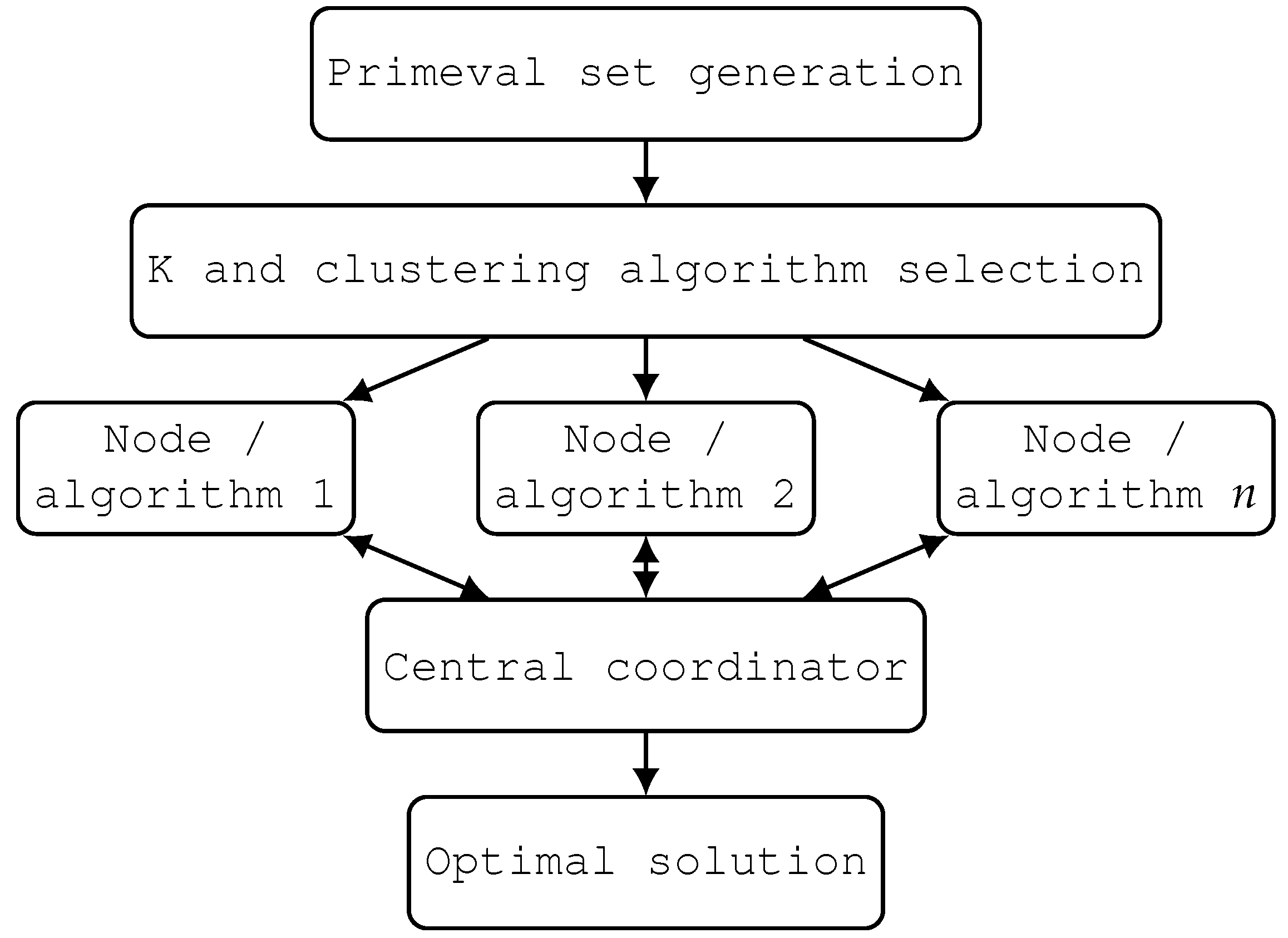
As mentioned above, a strategy has been established to enable collaboration levels between nodes and thus allow better results to be shared among different executions and nodes. The different nodes are triggered and coordinated by a central coordinator (CC), which iteratively receives the best found fitness for each performance—basically, a parameter set interval of iterations, in such a way that each node reports its best fitness to the CC and finds the best ones from all. Once determined, the CC distributes the selected best solutions toward all nodes, thus improving the quality of all searching spaces. The mechanism for the interaction between nodes is based on the periodic supervision of the results of each instance by the CC, which, in the event of a significant improvement in any of them, distributes part of the set of solutions with better fitness to the others. To achieve this, the algorithm’s executions are interrupted periodically after a certain number of iterations, according to a global parameter, to inform the CC of their results and the reception of a subset of better quality solutions found by another node, which contributes to enriching its own. The value of this parameter was experimentally established in 100 iterations, which has been repeated throughout the search process for all nodes. Once one of the nodes finds the global optimum or the exit criterion, the CC reviews the solutions found and delivers the found optimum, along with some other values. The Figure 1 shows this relationship:

Upon analysis of the figure from top to bottom, the generation of an extended set of feasible solutions called a “primeval set” is observed. The process continues by determining the clustering algorithm to use and the appropriate number of clusters to generate (K), as can see in the second stage. In general, different clustering algorithms can deliver different results for the same data [32]. Therefore, to ensure an adequate distribution of solutions, two data science algorithms were used, which were then compared: Kmeans [33] and agglomerative clustering [34]. This stage was only executed once centrally, requiring a minimum portion of time, with respect to the total time taken by the entire process. At runtime, it was determined which of the two methods is better balanced and distributed for different quantities of groups or clusters that are then generated in the third step. These clusters were then used as input to a MapReduce approach, making it responsible for parallelizing the search through different nodes. It was determined that at least the same number of nodes will be generated as clusters; thus, the number of nodes will always be greater than K. Each node executes a metaheuristic with its assigned group of solutions, while a central layer coordinates its operation. The solid red line represents the interactions of nodes with the CC every 100 iterations to report the results, and the dotted blue line represents the distribution of values selected by the CC. The use of parallel populations makes it possible to multiply the processing capacity, achieving optimal results in less time compared to a standalone architecture. Additionally, the distributed execution offers the possibility of dividing the search into different neighborhoods of solutions, increasing the exploration/exploitation capacity within the search process.

Best solutions are exchanged between nodes permanently over a set number of iterations. In the event that one of the nodes finds the global optimum, it will inform the CC at the end of the current set of iterations and the cluster runs will stop. On the other hand, those solutions closer to the global optimum will prevail as the iterations progress, since they will be distributed among the nodes and replace those with worse fitness. Then, the very mechanics of permanent exchange of better quality solutions causes that always the best fitness solutions found are present in all the nodes. Considering that the best solutions found replace the worst ones of the other nodes, the solutions of neighborhoods that so far are of regular or acceptable quality will be preserved, in order to stimulate the exploration in other neighborhoods while minimizing the stagnation in local solutions.

For each algorithm used, their respective parameters were determined experimentally by means of their standalone execution. The same values were then used in the distributed executions, in order to make possible the comparison of results between both modalities. We have illustrated notable improvements over a large instance set of the well-known NP-hard set covering problem, where the proposed approach is able to compete with other modern metaheuristics, while clearly outperforming the non-parallel version of some algorithms. Moreover, the framework presented is flexible enough to allow the addition of new algorithms, or replacing those used in this work. This is relevant, as the results show heterogeneous performance among the different algorithms.

3.2. Clustering

To separate the solutions into different groups, according to the described characteristics, the Kmeans [33] and agglomerative clustering [34] algorithms were used. The used clustering algorithms used are learning techniques based on model-free strategies, which do not require a training phase and can therefore be applied without the need for a prior representative sample of solutions for each algorithm. Both algorithms are commonly used unsupervised machine learning techniques know for being flexible, quick and reliable [35].

To use them, it is crucial to previously determine a value that corresponds to the number of clusters into which data will be divided. This number is represented by “K”. Both algorithms are executed, and their results are compared using the silhouette coefficient method [36] to determine the appropriate K value, and the algorithm that delivers the better results. Once the value of K is determined, the selected algorithm is applied to the entire initial set of solutions, assigning a cluster number to each of them.

Subsequently, the solutions are separated and grouped according to the assigned cluster, extracting the solutions needed to cover each one according to the initial parameter of each algorithm, similar to selecting the solutions of best fitness for each cluster. At this point, the distributed execution can start. The K nodes are generated and assigned one of the predefined algorithms: BBH, SLC, SFLA and SHO. If K is greater than the number of available algorithms (four in this research), the algorithms are repeated in a fixed sequence until the defined K is completed. The number of algorithms used is arbitrary and responds to tactical reasons, and there is no reason for there to be more of them.

4. Implemented Metaheuristics and Optimization Problem

For experimental purposes, we decided to tackle a well-known optimization problem to compare our results with previous results and have an abundant bibliography. For this reason, a classical NP-hard problem, the set covering problem (SCP), was selected. However, the proposed framework can be easily adapted to solve some other more complex modeling problems.

Regarding the algorithms used, four factors were considered: First, population algorithms were selected because they are more directly adaptable to the proposed architecture, although other types of algorithms can also be easily incorporated. Second, relatively modern algorithms with reported results were preferred in order to have a first-hand approximation of their effectiveness, and the recommended parameter values for each of them. Third, they were algorithms with differences in their convergence rates to determine if the variable is a relevant factor in the values obtained. Finally, considering that what we want to evaluate is the difference in behavior as a whole, and not the intrinsic nature and quality of each of them, we chose some that had already been used by researchers in the past, in order to facilitate their adaptation.

4.1. Set Covering Problem

Considering ($a_{ij}$) an binary array A defined by m rows and n columns, and a C vector ($c_j$) of n columns containing the costs assigned to each other, then we can then define the SCP as follows:

$${\displaystyle \mathrm{Minimize}\sum _{j=1}^n{c}_j{x}_j}$$

(1)

where:

$${\displaystyle \sum _{j=1}^n{a}_{ij}{x}_j\ge 1\forall i\in \{1,\dots ,m\}}$$

$$x_j\in \{0,1\};j\in \{1,\dots ,n\}$$

This ensures that each row is covered by at least one column where there is a cost associated with it. This problem was introduced in 1972 by Karp [37] and was used to optimize problems of element location that provide spatial coverage, such as community services [38], telecommunications antennas [39] and others [40].

4.2. Metaheuristics Implemented

The algorithms used in this work were selected based on two aspects. Firstly, they correspond to population algorithms of different complexities, from a very simple one such as BBH to others with more complex operators, such as SFLA and SHO. Secondly, the research team has several published works using these same algorithms, so the work of adaptation, tuning and comparison of results was relatively easy. Notwithstanding these observations, the work focuses on the collaborative and distributed execution of the algorithms and not on the nature, operators or parametrization of them, so that the proposed framework can be extended to many other algorithms, traditional or new.

4.2.1. Binary Black Hole Algorithm

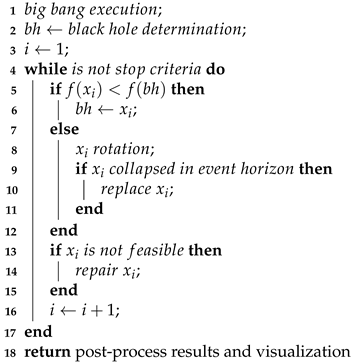
The binary black hole algorithm [4] faces the problem of determining solutions through the development of a set of stars called universe, using a population algorithm. It proposes the rotation of the universe around the star that has the best fitness, i.e., the one with lowest fitness value. This rotation is applied by an operator that moves each star in each iteration of the algorithm, and determines if there is a new black hole in each cycle. If it so happens, it replaces the previous one. This operation is repeated until the stop criterion is met, making the last black hole found the proposed final solution. Eventually, a star may exceed the distance defined by the radius of the event horizon. In this case, the star can collapse into a black hole and will be removed from the universe, substituted by a new star. The input for the algorithm are the universe size and max iterations, and the output is the last black hole found. The procedure can be seen in Algorithm 1.

Algorithm 1: Binary black hole algorithm.

4.2.2. Soccer League Competition Algorithm

Soccer league competition algorithm is a metaheuristic model based on soccer competitions [41]. This approach considers solutions as soccer players, and sets them up as soccer teams. There are movement operators applied to the players, emulating the dynamics generated in real matches to win and become the best football player of the season. Players are defined as two types: fixed players and substitutes ones. The convergence of the population towards the global optimum is achieved through competition among teams competing for the top positions in the classification table. Players also compete to be fixed and be the star ones of their respective teams. The goal is to find the best feasible solution that achieves the best value from the evaluation function, using operators who evaluate the players and teams’ performances and exchange solutions. The algorithm inputs are the number of teams and fixed and substitute players. The output is the star player. Algorithm 2 details the resolution process.

Algorithm 2: Soccer league competition algorithm.

4.2.3. Shuffled Frog-Leaping Algorithm

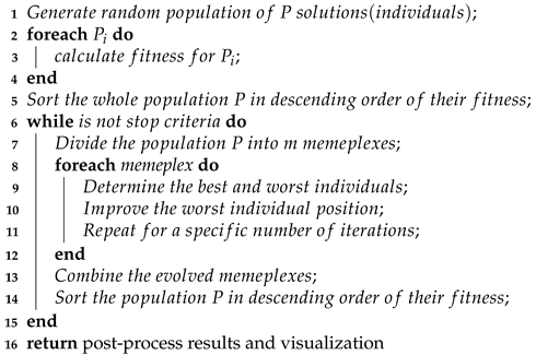
The shuffled frog leaping algorithm is a population-based cooperative search metaheuristic, inspired by natural memetics [6]. The algorithm manages a set of interacting virtual population of frogs, partitioned into different memeplexes, including elements of local search and global information exchange. The frogs simulate hosts of memes, where a meme is a basic unit of cultural evolution. This algorithm performs independent local searches on each memeplex, using a variant of the particle swarm optimization method. The frogs are shuffled periodically and reorganized into new memeplexes. This technique is similar to that used in the complex evolutionary shuffle algorithm, to ensure global exploration. To improve randomness, frogs are randomly generated and replaced in the population. The algorithm input are the number of memeplexes, frogs in each memeplex, iterations in each memeplex and maximum algorithm iterations, while the output is the best frog fitness. Algorithm 3 explains the step-by-step of the resolution process.

Algorithm 3: Shuffled frog leaping algorithm.

4.2.4. Spotted Hyena Optimizer Algorithm

The fundamental concept of this algorithm is the natural hunting strategy of the spotted hyena [7]. The three basic steps of this proposed spotted hyena optimizer algorithm are searching, encircling, and attacking for prey. Spotted hyenas first search for prey, depending on their position residing in the solution space, and then move away from each other to attack their prey.

Similarly, we use operators with random values to force the search agents to move far away from the prey, thereby stimulating the SHO algorithm to search globally. To encircle the prey, the best solution is considered the target prey, and the other search agents or spotted hyenas can update their positions according to this optimal solution. The other search agents will try to update their positions after the best search candidate solution is defined. The third step of SHO algorithm is the attack strategy, which sets up a cluster of optimal solutions against the best search agent, and updates the positions of other search agents. The input for algorithm is the population $P_i$$(i=1,2,\dots ,n)$ and the output is the best search agent. Algorithm 4 presents the search process.

Algorithm 4: Spotted Hyena Optimizer algorithm.

5. Metodology

5.1. Platform

The Amazon elastic cloud (EC2) platform was used as the experimental environment for both modalities, configuring two-processor machines with 8 GB of RAM memory. In case of the distributed version, an equivalent virtual machine was implemented for each node. Each of them was executed separately, and the parameter setting was determined experimentally for each instance group. They were selected according to

Table 1. Algorithms main parameters.

BBH		SHO		SLC		SFLA
Parameter	Value	Parameter	Value	Parameter	Value	Parameter	Value
Universe size	70	Hyenas quantity	40	Teams quantity	10	Memeplex quantity	8
Max iterations	10,000	Max iterations	10,000	Max iterations	10,000	Frogs in memeplex	8
				Fixed players	6	Iter. memeplex	30
				Suplent players	5	Max iterations	10,000
				Im. factor	5
				Mult. factor	5
				Reduction	15
				Sust. factor	50

.

The algorithms were written in Python 3.7, and the experiments were conducted for NR instances, proposed by the OR-Library [42] for the SCP (NRE to NRH). They instances consisted of datasets of 500 × 5000 and 1000 × 10,000 lines and columns, respectively, and they were unicost problems from [43]. The results obtained by standalone algorithms were taken as a basis for comparison to those that were subsequently generated with the distributed framework. The analysis was focused on this comparison, and not on improving results by tuning the parameters or modifying the operators. Once the standalone experiments were completed, the distributed experiments were run on the Spark 2.2.3, platform with the same parameters. As mentioned above, the execution was collective, i.e., all nodes participated in a coordinated way in the searching for best solutions, reporting results to the CC every 100 iterations. This value was determined experimentally, and it corresponds to the approximate average number of iterations in which the four algorithms show improvements in searching. If new algorithms are incorporated or proposed, or they are replaced, the value of this parameter should be reevaluated. This collaboration among different algorithms means that the optimum found is a consequence of the search in different neighborhoods, carried out by different algorithms. Therefore, it does not correspond to a single metaheuristic, even if it is a particular one that finds the best value.

5.2. Experimental Design

Considering that the nodes of the distributed platform execute the same versions of the standalone algorithms, the improvement can be interpreted mainly as a product of two aspects of the proposed architecture: the clustering of the search space, and the collaboration among nodes. The resolution time and the number of calls to the objective function are variables subject to several conditions that make them not very objective. However, because the standalone and distributed experiments were run in similar environments and platforms, it is relevant to explain them.

The standalone experiments were performed by grouping by each of the instances and algorithms, i.e., 80 modalities that were run 31 times each, totaling 2480 experiments. In addition, the distributed version was run 31 times for each instance, i.e., 620 experiments.

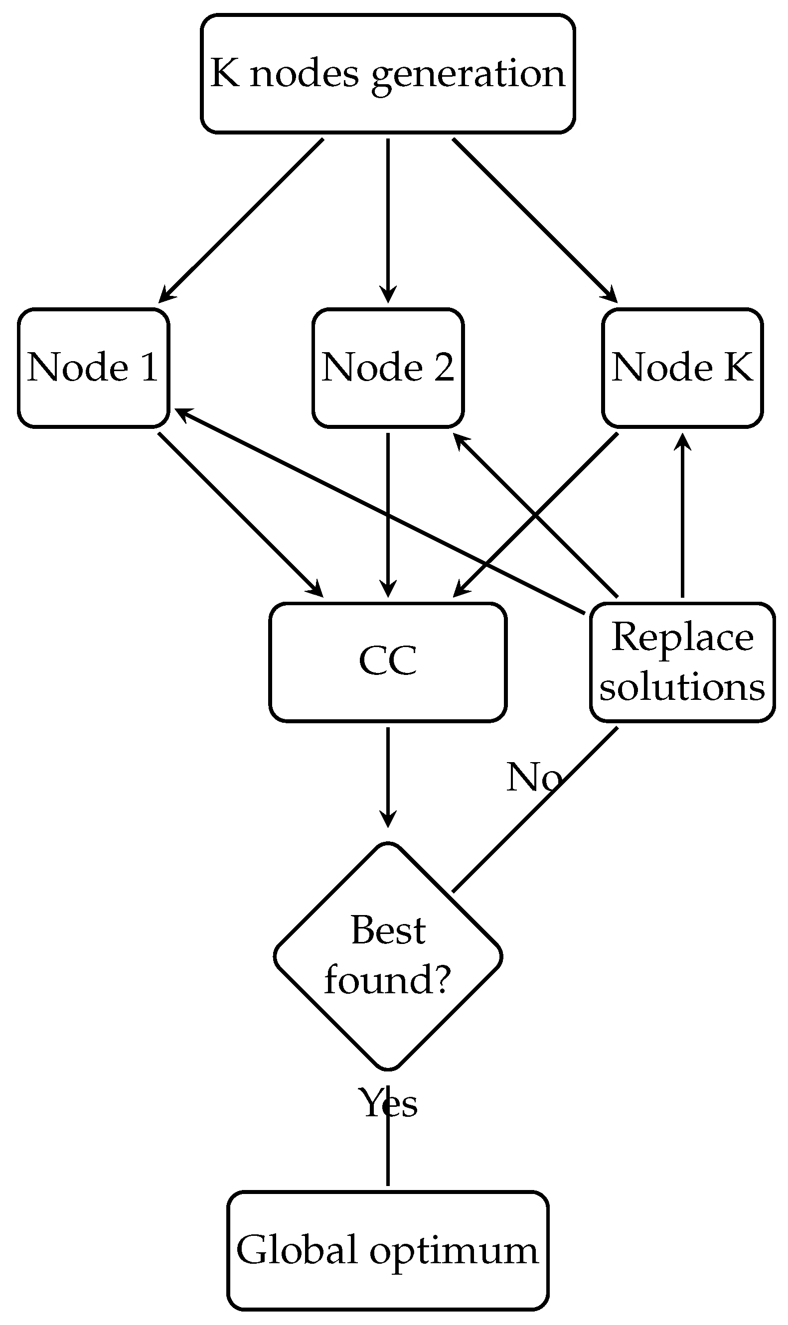
Because the proposed method is not metaheuristic itself, but the coordinated work of several of them, it becomes relevant to figure out the contribution of each one in the complete search towards the optimum value. As noted above, every 100 iterations, the algorithms reported the best solution found to the CC. If this solution was better than the current optimal, the other algorithms were informed of the same, we can observe this behavior in the Figure 2.

If we consider the existing iterations since the previous optimum was received, and the new one that was found in an algorithm as collaboration time, we can quantify the percentage of participation for each algorithm in the search process. In the same way, it is important to know the behavior of this collaboration for different algorithms, in different stages of the search. For better analysis, the entire search process was divided into deciles.

To determine how decisive the number of nodes generated is in the results obtained, the experiments were replicated in three modalities. The first method consisted of generating K nodes, i.e., a unique node for each cluster. The second one consisted the generation of 2K nodes. In other words, two nodes for each detected cluster. The third one, in analogy, corresponded to the generation of 3K nodes.

Because K is generally larger than the number of used algorithms, for each round of experiments, the algorithms were assigned in fixed sequence, i.e., for K = 4, each cluster was addressed by a different algorithm, and for k > 4, the algorithms started repeating in a fixed order.

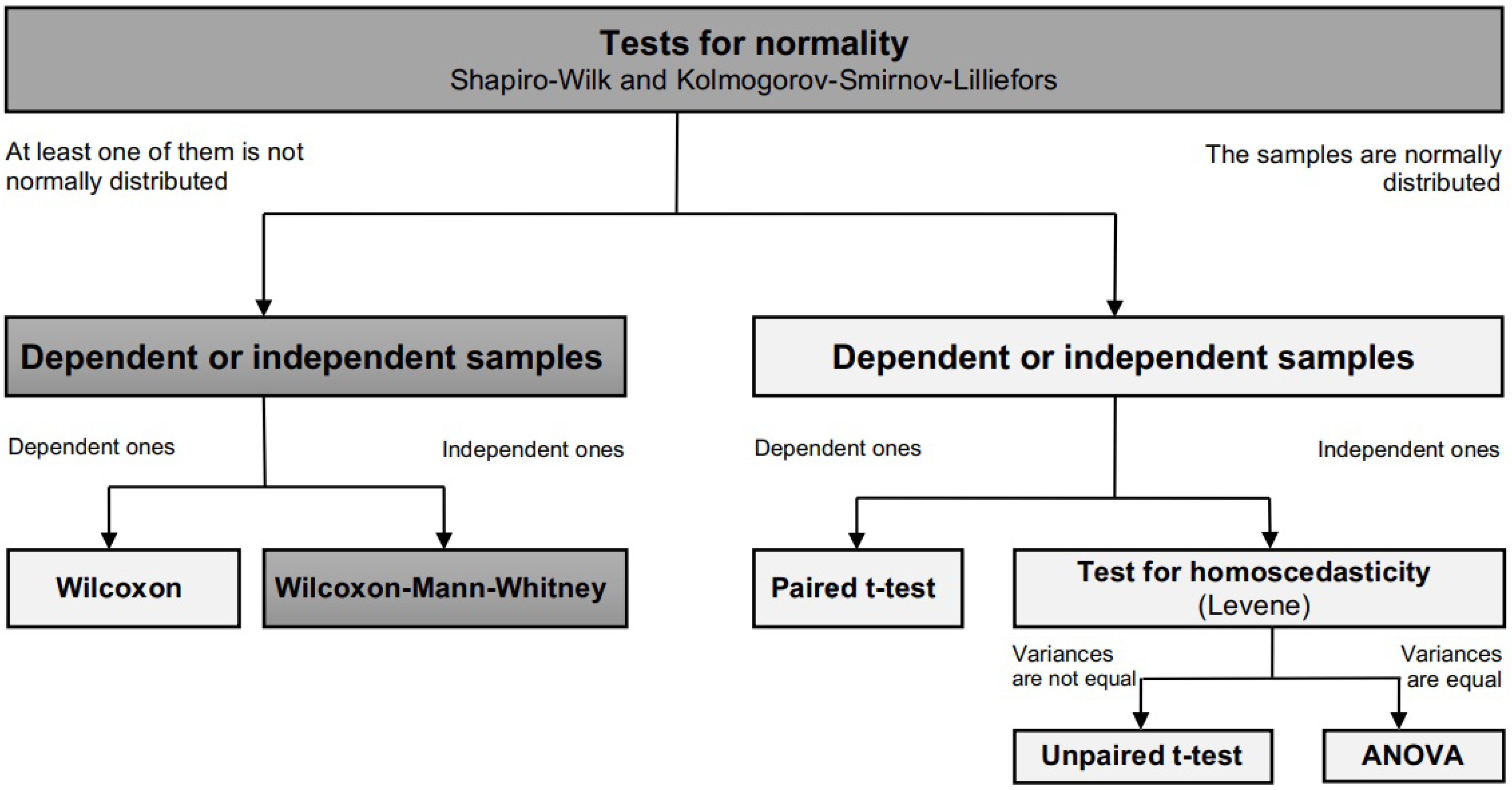
6. Statistical Analysis

Due to the stochastic nature of metaheuristics, it is not sufficient to present good results about the optimums found; it is important to demonstrate statistical regularity of the obtained values as well. This can be explained by results which do not necessarily satisfy qualities such as normality, homoscedasticity and independence, as demonstrated by [44,45]. For this purpose, Lanza and Gómez [46] proposed a methodology to compare two algorithms, or variations of them, considering the regularity and consistency of results. The details can be seen in the Figure 3:

The first step was to determine the outliers in the results of each algorithm, for all instances used. For this purpose, the average result for each of the experiments were calculated for every instance. The first and third quartiles and the interquartile range were calculated next. In the cases in which extreme outliers were found, these values were eliminated from the results table, leaving only the mild ones to be analyzed. The next steps were to determine the data distribution and independence, i.e., whether it has normal distribution or can be considered statistically belonging to different sets. For the first, the Shapiro–Wilk and Kolmogorov–Smirnov–Lilliefors tests were applied to detect the normality of the results. These tests were raised for the four algorithms used, and also for the distributed execution. To determine whether the proposed architecture was more regular and statistically coherent than each of the standalone algorithms, the Wilcoxon and Wilcoxon–Mann–Whitney tests were applied to the paired and independent datasets, respectively. This method was applied to each sequence of experiments in the three modalities described in the previous section.

7. Experimental Results

Table 2. Results comparison for standalone versions.

Instance	${\mathit{Z}}_{\mathit{BKS}}$	${\mathit{Min}}_{\mathit{SFLA}}$	${\mathit{RPD}}_{\mathit{SFLA}}$	${\mathit{Min}}_{\mathit{SHO}}$	${\mathit{RPD}}_{\mathit{SHO}}$	${\mathit{Min}}_{\mathit{SLC}}$	${\mathit{RPD}}_{\mathit{SLC}}$	${\mathit{Min}}_{\mathit{BBH}}$	${\mathit{RPD}}_{\mathit{BBH}}$
NRE1	29	41	41.38	29	0.00	34	17.24	52	79.31
NRE2	30	31	3.33	32	6.67	37	23.33	46	53.33
NRE3	27	38	40.74	29	7.41	38	40.74	28	3.70
NRE4	28	40	42.86	32	14.29	31	10.71	29	3.57
NRE5	28	41	46.43	28	0.00	39	39.29	28	0.00
NRF1	14	14	0.00	18	28.57	23	64.29	17	21.43
NRF2	15	18	20.00	15	0.00	18	20.00	18	20.00
NRF3	14	16	14.29	14	0.00	20	42.86	14	0.00
NRF4	14	15	7.14	15	7.14	18	28.57	16	14.29
NRF5	13	16	23.08	14	7.69	17	30.77	14	7.69
NRG1	176	201	14.20	190	7.95	185	5.11	180	2.27
NRG2	151	166	9.93	158	4.64	176	16.56	153	1.32
NRG3	166	170	2.41	170	2.41	173	4.22	166	0.00
NRG4	168	169	0.60	170	1.19	181	7.74	197	17.26
NRG5	168	183	8.93	169	0.60	189	12.50	171	1.79
NRH1	63	68	7.94	66	4.76	69	9.52	71	12.70
NRH2	63	69	9.52	66	4.76	66	4.76	70	11.11
NRH3	59	63	6.78	59	0.00	66	11.86	67	13.56
NRH4	59	73	23.73	61	3.39	62	5.08	69	16.95
NRH5	55	70	27.27	58	5.45	61	10.91	64	16.36

shows the best results obtained for each instance of the set covering problem. These are highlighted in bold font. $Z_{BKS}$ is the known global optimum for each instance, while $Mi{n}_{SFLA}$, $Mi{n}_{SHO}$, $Mi{n}_{SLC}$ and $Mi{n}_{BBH}$ were the best values obtained for each instance by the standalone algorithms. The RPD in each experiment group is the relative percentage deviation from the known optimum, calculated as follows: $\left(\frac{Mi{n}_{found}\ast 100}{Z_{bks}}\right)-100$.

For the following tables, we report the $Mi{n}_{DT}$, $Ma{x}_{DT}$, $Me{d}_{DT}$ and $RP{D}_{DT}$ columns that show the minimum, maximum, median and RPD values obtained with the proposed framekork (DT).

Table 3. K nodes RPD comparison for standalone and distributed versions.

Instance	BKS	${\mathit{Min}}_{\mathit{DT}}$	${\mathit{Max}}_{\mathit{DT}}$	${\mathit{Med}}_{\mathit{DT}}$	${\mathit{RPD}}_{\mathit{DT}}$	${\mathit{RPD}}_{\mathit{SFLA}}$	${\mathit{RPD}}_{\mathit{SHO}}$	${\mathit{RPD}}_{\mathit{SLC}}$	${\mathit{RPD}}_{\mathit{BBH}}$	MFE	CT
NRE1	29	29	55	43	0.00	41.38	0.00	17.24	79.31	1,071,926	2.060
NRE2	30	32	58	49	6.67	3.33	6.67	23.33	53.33	1,068,618	2.054
NRE3	27	28	33	30	3.70	40.74	7.41	40.74	3.70	1,000,391	1.923
NRE4	28	29	56	46	3.57	42.86	14.29	10.71	3.57	922,880	1.774
NRE5	28	28	61	47	0.00	46.43	0.00	39.29	0.00	960,027	1845
NRF1	14	15	35	24	7.14	0.00	28.57	64.29	21.43	1,071,669	1600
NRF2	15	15	29	23	0.00	20.00	0.00	20.00	20.00	1,158,639	1729
NRF3	14	14	25	22	0.00	14.29	0.00	42.86	0.00	1,131,867	1689
NRF4	14	15	22	19	7.14	7.14	7.14	28.57	14.29	1,225,920	1830
NRF5	13	14	27	23	7.69	23.08	7.69	30.77	7.69	1,282,364	1915
NRG1	176	178	219	195	1.14	14.20	7.95	5.11	2.27	876,533	2020
NRG2	151	153	190	172	1.32	9.93	4.64	16.56	1.32	952,975	2197
NRG3	166	172	199	182	3.61	2.41	2.41	4.22	0.00	966,945	2228
NRG4	168	174	205	191	3.57	0.60	1.19	7.74	17.26	897,329	2069
NRG5	168	175	226	201	4.17	8.93	0.60	12.50	1.79	929,964	2143
NRH1	63	66	83	75	4.76	7.94	4.76	9.52	12.70	968,004	1940
NRH2	63	65	85	74	3.17	9.52	4.76	4.76	11.11	1,052,336	2109
NRH3	59	59	94	81	0.00	6.78	0.00	11.86	13.56	1,018,750	2042
NRH4	59	63	100	83	6.78	23.73	3.39	5.08	16.95	989,600	1983
NRH5	55	57	101	77	3.64	27.27	5.45	10.91	16.36	1,050,947	2.106
AVG					3.40	17.53	5.35	20.30	14.83	1,029,884	1963

shows the best results obtained for each SCP benchmark by the version distributed on K nodes, compared to the RPDs with those of the standalone versions. Again, the best results are highlighted in bold font. The MFE corresponds to the number of evaluations performed of the objective function, and CT is the computation time in minutes for total execution.

Table 4. 2K nodes RPD comparison for standalone and distributed versions.

Instance	BKS	${\mathit{Min}}_{\mathit{DT}}$	${\mathit{Max}}_{\mathit{DT}}$	${\mathit{Med}}_{\mathit{DT}}$	${\mathit{RPD}}_{\mathit{DT}}$	${\mathit{RPD}}_{\mathit{SFLA}}$	${\mathit{RPD}}_{\mathit{SHO}}$	${\mathit{RPD}}_{\mathit{SLC}}$	${\mathit{RPD}}_{\mathit{BBH}}$	MFE	CT
NRE1	29	29	55	42	0.00	41.38	0.00	17.24	79.31	2,004,884	2.493
NRE2	30	31	52	41	3.33	3.33	6.67	23.33	53.33	2,033,992	2378
NRE3	27	28	33	30	3.70	40.74	7.41	40.74	3.70	1,999,607	2490
NRE4	28	29	48	39	3.57	42.86	14.29	10.71	3.57	1,772,022	1952
NRE5	28	28	44	36	0.00	46.43	0.00	39.29	0.00	1,908,427	2156
NRF1	14	15	29	22	7.14	0.00	28.57	64.29	21.43	2,051,072	1698
NRF2	15	15	30	22	0.00	20.00	0.00	20.00	20.00	2,137,033	1657
NRF3	14	15	25	20	7.14	14.29	0.00	42.86	0.00	2,226,238	1851
NRF4	14	14	21	18	0.00	7.14	7.14	28.57	14.29	2,299,324	2301
NRF5	13	14	25	20	7.69	23.08	7.69	30.77	7.69	2,286,180	2488
NRG1	176	177	201	189	0.57	14.20	7.95	5.11	2.27	1,597,704	2497
NRG2	151	151	190	172	0.00	9.93	4.64	16.56	1.32	1,549,860	2.517
NRG3	166	170	187	179	2.41	2.41	2.41	4.22	0.00	1,592,800	3088
NRG4	168	171	176	174	1.79	0.60	1.19	7.74	17.26	1,586,827	2515
NRG5	168	169	201	185	0.60	8.93	0.60	12.50	1.79	1,514,488	2908
NRH1	63	65	83	74	3.17	7.94	4.76	9.52	12.70	1,901,904	2324
NRH2	63	65	80	72	3.17	9.52	4.76	4.76	11.11	1,931,757	2447
NRH3	59	59	79	69	0.00	6.78	0.00	11.86	13.56	1,867,105	2615
NRH4	59	62	94	78	5.08	23.73	3.39	5.08	16.95	1,849,555	2596
NRH5	55	56	77	67	1.82	27.27	5.45	10.91	16.36	1,922,298	2.839
AVG					2.56	17.53	5.35	20.30	14.83	1,901,654	2391

and

Table 5. 3K nodes RPD comparison for standalone and distributed versions.

Instance	BKS	${\mathit{Min}}_{\mathit{DT}}$	${\mathit{Max}}_{\mathit{DT}}$	${\mathit{Med}}_{\mathit{DT}}$	${\mathit{RPD}}_{\mathit{DT}}$	${\mathit{RPD}}_{\mathit{SFLA}}$	${\mathit{RPD}}_{\mathit{SHO}}$	${\mathit{RPD}}_{\mathit{SLC}}$	${\mathit{RPD}}_{\mathit{BBH}}$	MFE	CT
NRE1	29	29	52	41	0.00	41.38	0.00	17.24	79.31	2,909,407	2.735
NRE2	30	31	52	42	3.33	3.33	6.67	23.33	53.33	2,827,970	2640
NRE3	27	28	32	30	3.70	40.74	7.41	40.74	3.70	2,747,377	2527
NRE4	28	29	48	39	3.57	42.86	14.29	10.71	3.57	2,589,137	1900
NRE5	28	28	41	35	0.00	46.43	0.00	39.29	0.00	2,719,367	2159
NRF1	14	15	29	22	7.14	0.00	28.57	64.29	21.43	2,899,910	1449
NRF2	15	15	30	23	0.00	20.00	0.00	20.00	20.00	2,826,411	1611
NRF3	14	14	22	18	0.00	14.29	0.00	42.86	0.00	2,904,276	1697
NRF4	14	14	20	17	0.00	7.14	7.14	28.57	14.29	2,829,308	2246
NRF5	13	14	25	20	7.69	23.08	7.69	30.77	7.69	2,734,454	2514
NRG1	176	176	196	186	0.00	14.20	7.95	5.11	2.27	2,551,637	2678
NRG2	151	154	188	171	1.99	9.93	4.64	16.56	1.32	2,645,503	2958
NRG3	166	170	187	179	2.41	2.41	2.41	4.22	0.00	2,635,247	3433
NRG4	168	171	176	174	1.79	0.60	1.19	7.74	17.26	2,688,812	2764
NRG5	168	169	201	185	0.60	8.93	0.60	12.50	1.79	2,786,969	3171
NRH1	63	65	80	73	3.17	7.94	4.76	9.52	12.70	2,891,291	2428
NRH2	63	65	79	72	3.17	9.52	4.76	4.76	11.11	2,891,423	2774
NRH3	59	59	77	68	0.00	6.78	0.00	11.86	13.56	2,946,120	2799
NRH4	59	61	90	76	3.39	23.73	3.39	5.08	16.95	2,778,388	2696
NRH5	55	55	76	66	0.00	27.27	5.45	10.91	16.36	3,001,766	3063
AVG					2.10	17.53	5.35	20.30	14.83	2,790,239	2512

show results for the execution with 2K nodes and 3K node, respectively. We employed bold font to illustrate the best results, again. In the resolved benchmarks, it is possible to notice a greater difference in the RPDs obtained, as well as in the number of found global optimums. This is relevant, since these instances represent types of problems that present difficulties in being solved using metaheuristics and demand higher computational power due to the large volume of data.

For the standalone versions of the SFLA, SHO, SLC and BBH algorithms, the average RPDs are 17.53, 5.35, 20.30 and 14.83, respectively, but for the distributed (DT) K, 2K and 3K versions, they are 3.40, 2.56 and 2.10, respectively, which are significantly lower. It is clear from the above tables that for the K, 2K and 3K node versions, 60%, 80% and 80%, respectively, of the instances performed as well or better in the DT architecture than in any of the standalone algorithms. 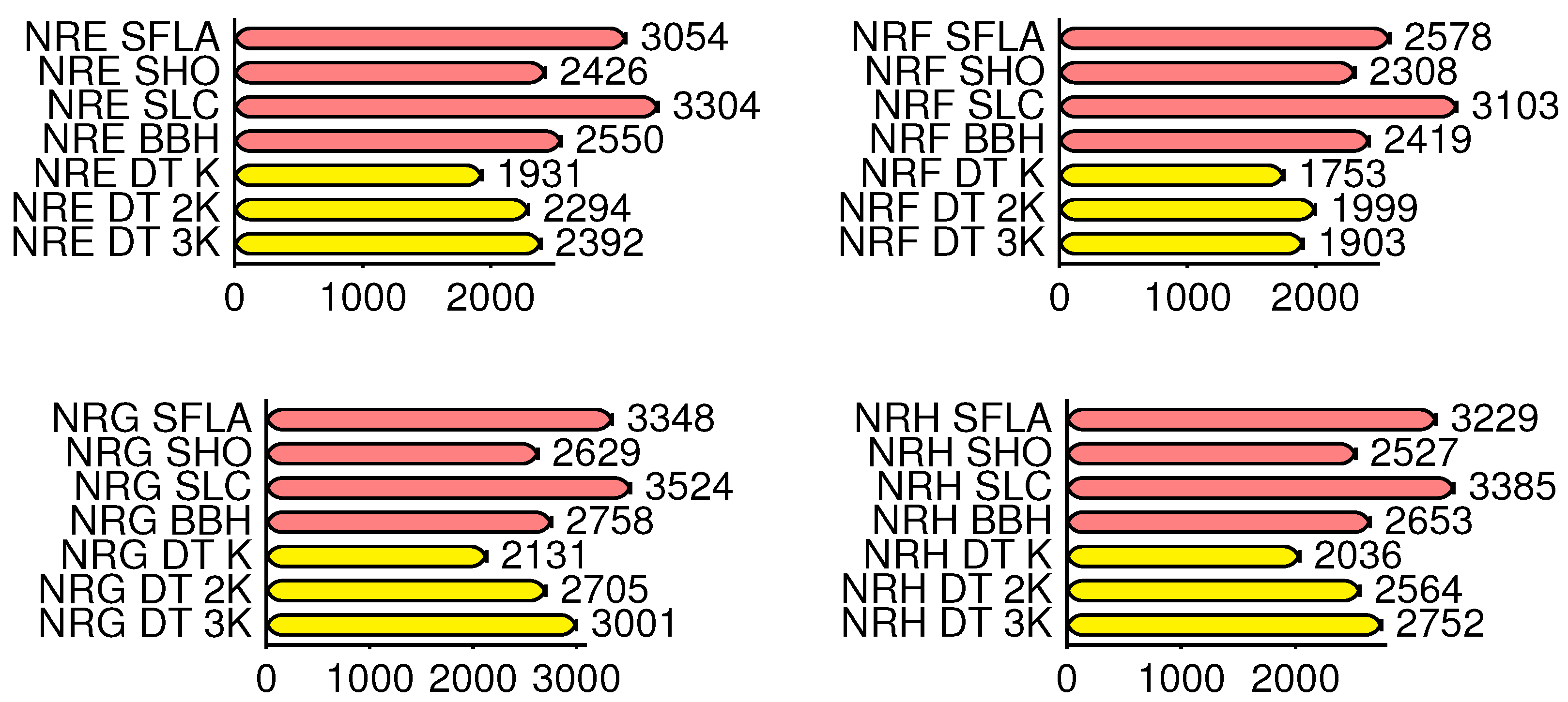Figure 4 shows the average times in minutes used by the autonomous and DT algorithms that find the minimum values of some instances, or the output criteria, grouped by instance type.

The above graphs show that the proposed architecture, on average, always solved the instances in less computational time than the best standalone algorithm.

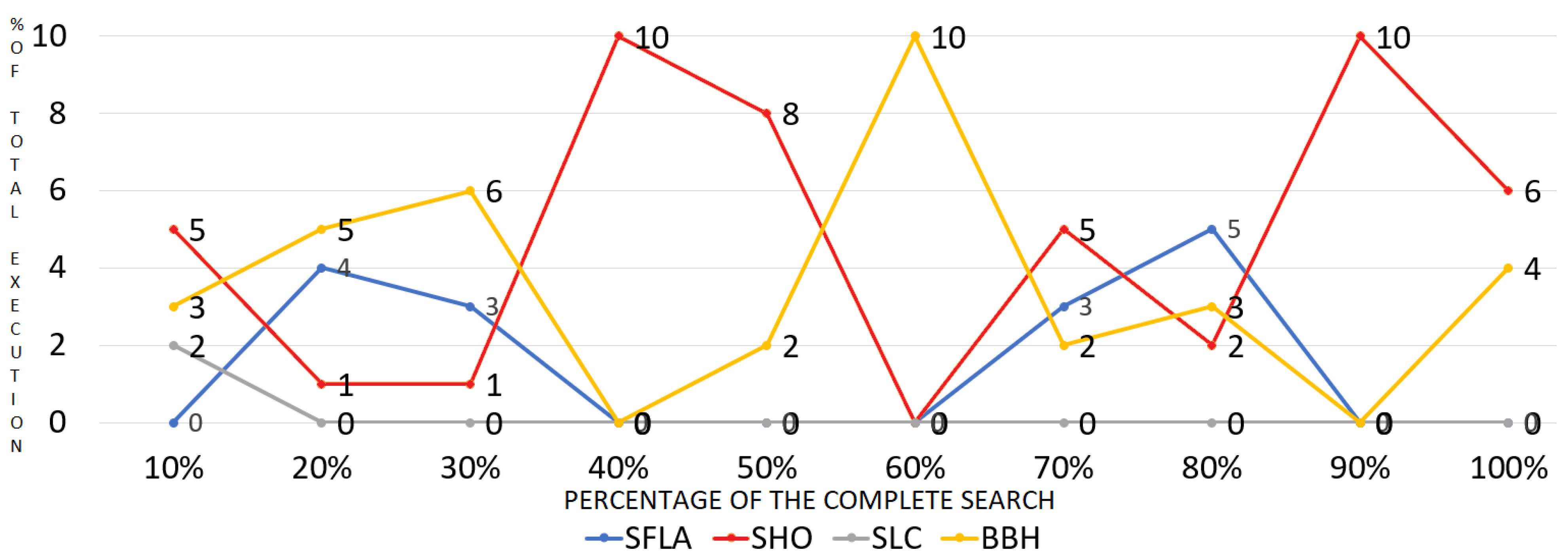
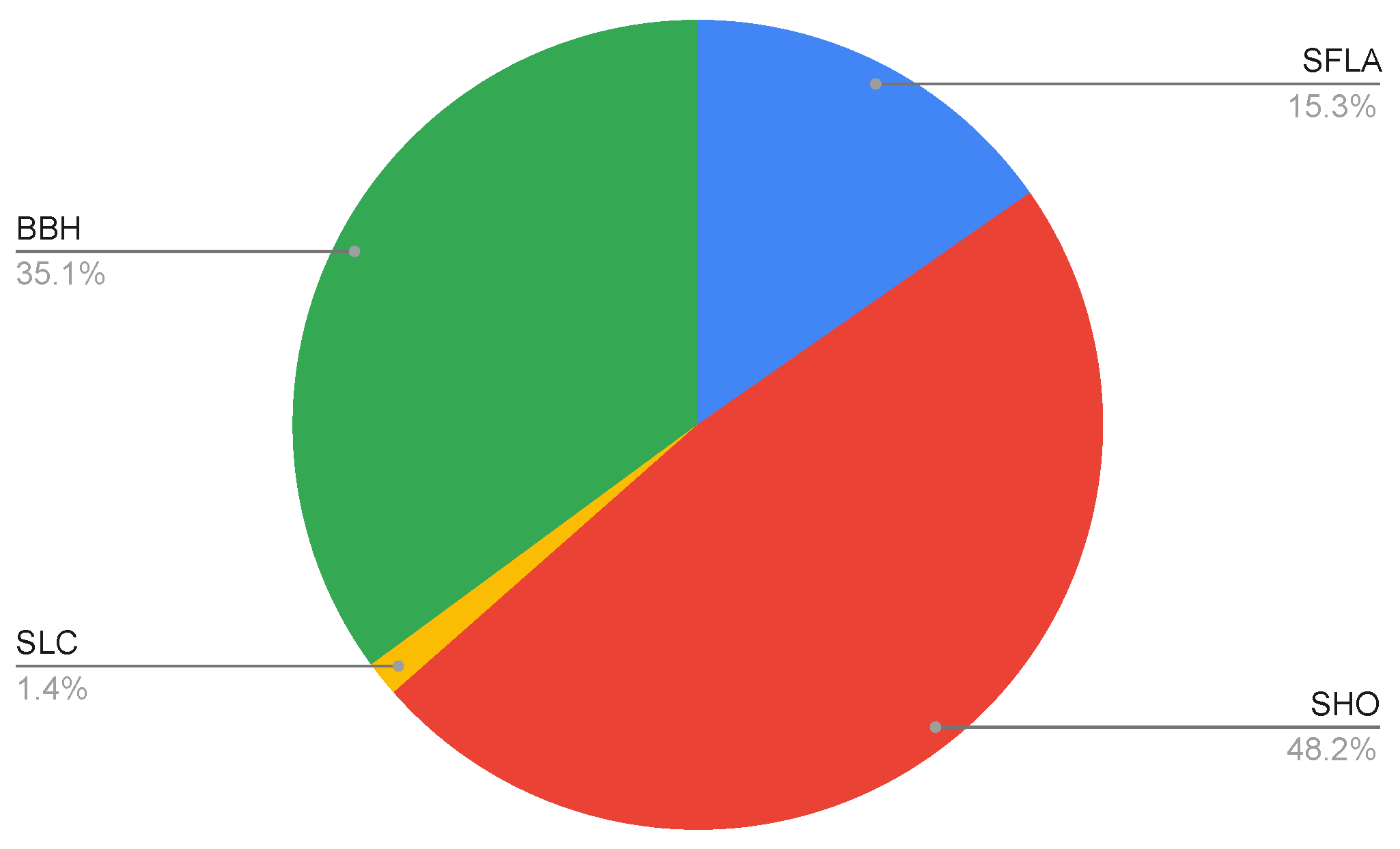
Figure 5 shows how the average percentage of collaboration is distributed for each algorithm, considering all the resolved instances.

In Figure 6, the percentage of participation for each algorithm in each decile X-axis is represented on the Y-axis, so it is easy to observe the importance of each algorithm in all stages of the search.

As it can be observed, the SHO and BBH algorithms participate in most of the optimum searches. The SFLA participates only partially, and the SLC only participates during the first iterations. One of the factors that explains this is the difference in the convergence rates of the algorithms. Those that converge faster have greater collaboration, but when the convergence rates of the algorithms are relatively similar, collaboration must be encouraged. This is the case for the SHO and BBH algorithms, which have similar convergence rates and cooperate with each other for most of the process, as opposed to the SLC, which has a very slow convergence.

To show the different convergence rates of each algorithm and the DT version, Figure 7 plots the evolution of the minimums found in each iteration, for each algorithm, for one of the solved instances. The rest of the instances presented the same behavior, with small differences of low significance.

Statistical Analysis

With these results, a table was constructed to determine the outliers, according to the following conditions:

$$Mildoutlier:value<Q_1-\left(1.5IQR\right)or>Q_3+\left(1.5IQR\right)$$

$$Extremeoutlier:value<Q_1-\left(3IQR\right)or>Q_3+\left(3IQR\right)$$

All the experiments had a p-value < 0.05. Therefore, it cannot be assumed that H0 was satisfied for any of the instances or algorithms. Similarly, their non-normal distribution was validated, and the independence of the results obtained was tested, resulting in most of them being independent, although a few were classified as dependent. According to the methodology detailed above, it is necessary to determine the statistical consistency of the independent and DT algorithms by applying the Wilcoxon and Wilcoxon–Mann–Whitney tests to the paired and independent datasets, respectively. The analysis was performed with the DT with K, 2K and 3K nodes, but since the statistical results between them were not significantly different, we show the values obtained with K nodes.

Table 6. Algorithm selected for tested instances.

SFLA-DT				SHO-DT
Instance	Selected	Instance	Selected	Instance	Selected	Instance	Selected
NRE1	SFLA	NRG1	DT	NRE1	DT	NRG1	DT
NRE2	DT	NRG2	SFLA	NRE2	SHO	NRG2	SHO
NRE3	DT	NRG3	DT	NRE3	SHO	NRG3	DT
NRE4	SFLA	NRG4	ND	NRE4	DT	NRG4	ND
NRE5	ND	NRG5	DT	NRE5	DT	NRG5	DT
NRF1	DT	NRH1	DT	NRF1	SHO	NRH1	SHO
NRF2	DT	NRH2	DT	NRF2	SHO	NRH2	DT
NRF3	DT	NRH3	DT	NRF3	DT	NRH3	SHO
NRF4	DT	NRH4	DT	NRF4	DT	NRH4	DT
NRF5	DT	NRH5	DT	NRF5	DT	NRH5	DT
SCL-DT				BBH-DT
Instance	Selected	Instance	Selected	Instance	Selected	Instance	Selected
NRE1	ND	NRG1	DT	NRE1	BBH	NRG1	DT
NRE2	SLC	NRG2	DT	NRE2	DT	NRG2	DT
NRE3	DT	NRG3	DT	NRE3	DT	NRG3	DT
NRE4	SLC	NRG4	DT	NRE4	DT	NRG4	DT
NRE5	DT	NRG5	DT	NRE5	DT	NRG5	DT
NRF1	DT	NRH1	DT	NRF1	ND	NRH1	DT
NRF2	DT	NRH2	ND	NRF2	DT	NRH2	BBH
NRF3	DT	NRH3	DT	NRF3	DT	NRH3	BBH
NRF4	DT	NRH4	DT	NRF4	ND	NRH4	BBH
NRF5	DT	NRH5	DT	NRF5	DT	NRH5	DT

shows the algorithm selected for all tested instances.

Figure 8 compares the global results distribution for statistical analysis. Almost three quarters of instances have better statistical regularity in the distributed algorithm.

Table 7. Results algorithm comparison.

Instance	SA	DT	Selected		Instance	SA	DT	Selected
NRE1	SHO	SHO	SFLA		NRG1	SHO	SHO	DT
NRE2	SFLA	SHO	DT		NRG2	BBH	BBH	SFLA
NRE3	BBH	BBH	DT		NRG3	SHO	SHO	DT
NRE4	SHO	SHO	SFLA		NRG4	SHO	BBH	ND
NRE5	SHO	SHO	ND		NRG5	SHO	SHO	DT
NRF1	SHO	BBH	DT		NRH1	BBH	BBH	DT
NRF2	SHO	SHO	DT		NRH2	SHO	SHO	DT
NRF3	BBH	BBH	DT		NRH3	SHO	BBH	DT
NRF4	SHO	SHO	DT		NRH4	SHO	SHO	DT
NRF5	SHO	SHO	DT		NRH5	SHO	BBH	DT

compares the instances detailing the standalone and DT algorithms with the best resultsas well as the statistically selected ones. In those cases in which the first two concur, the respective line is noted (ND = no difference). We can observe that in 75% of the instances, there is a coincidence in the algorithm that reports the best result, regardless of which is statistically the best.

We can observe that in 75% of the instances there is a coincidence in the algorithm that reports the best result, regardless of which is selected as the best statistically.

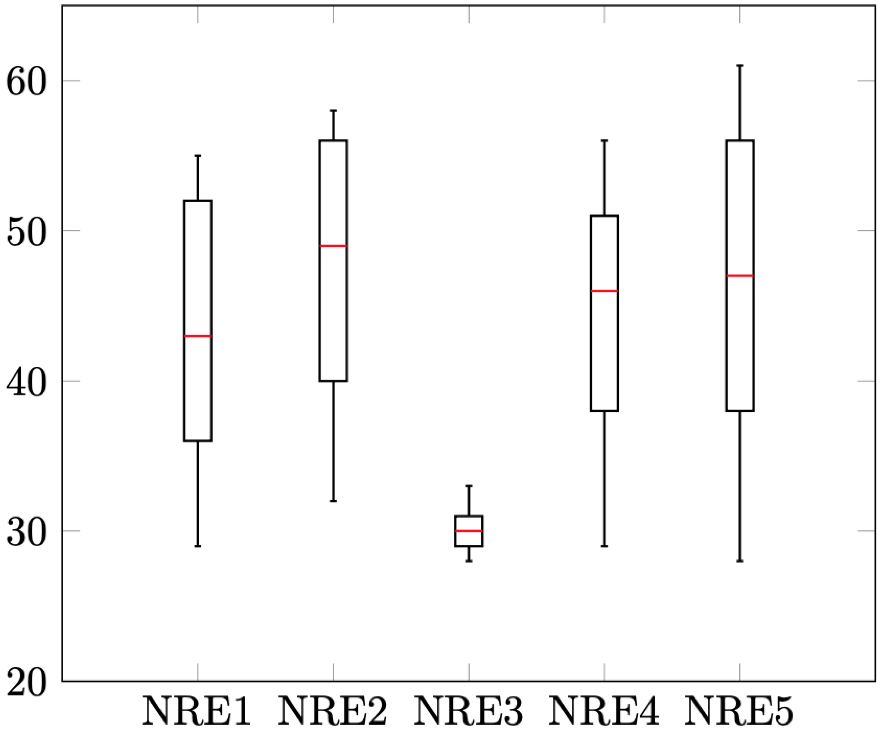
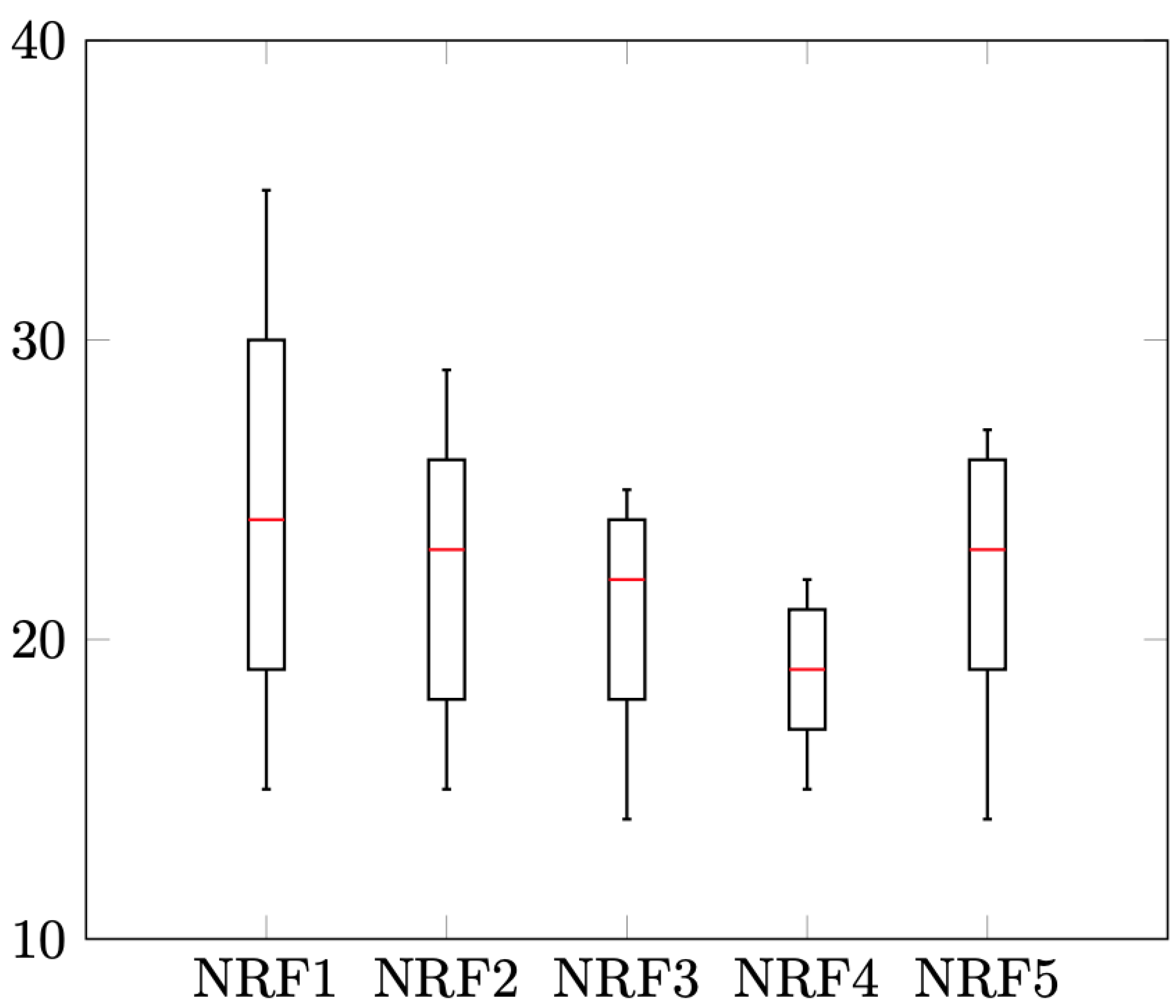
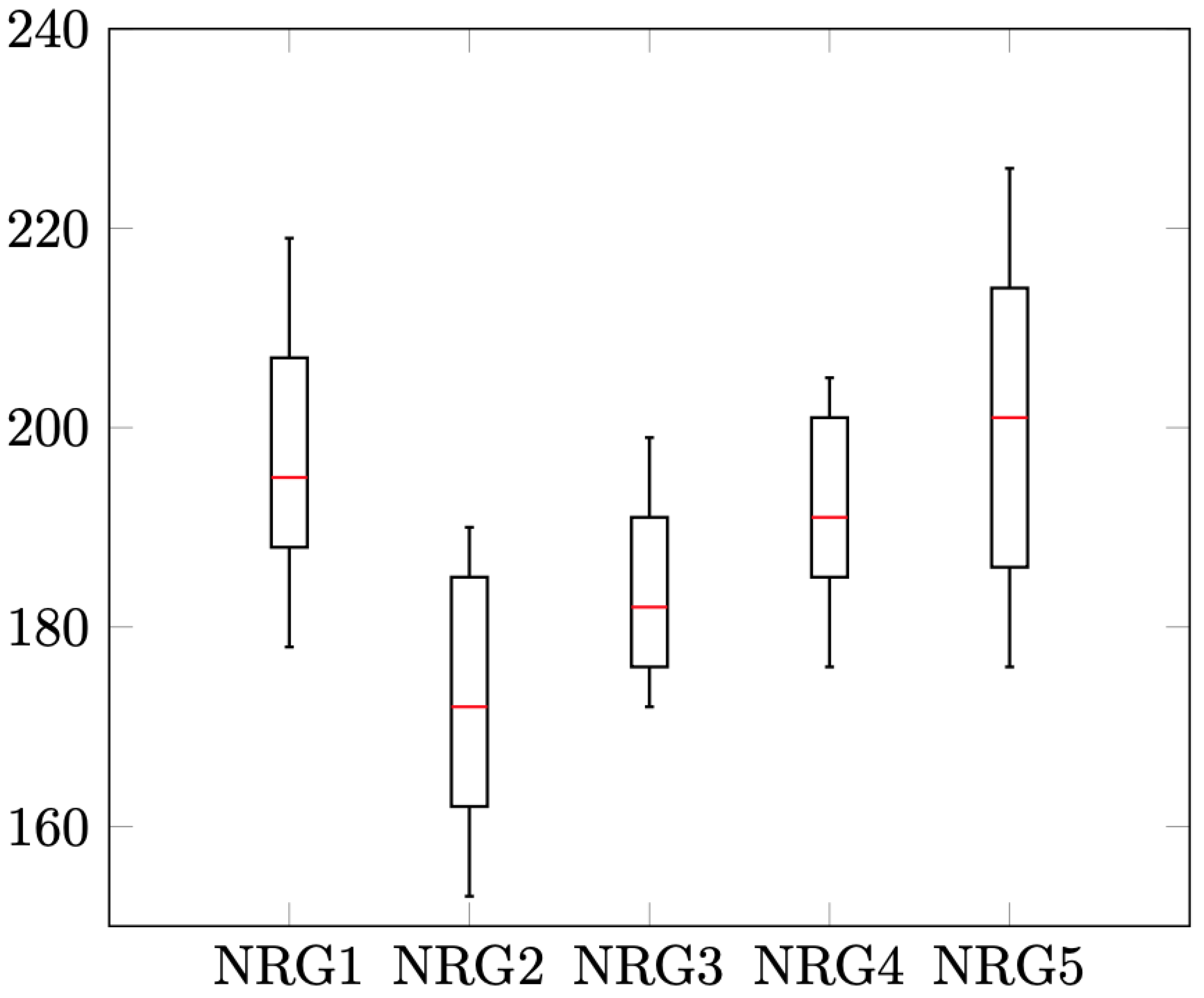
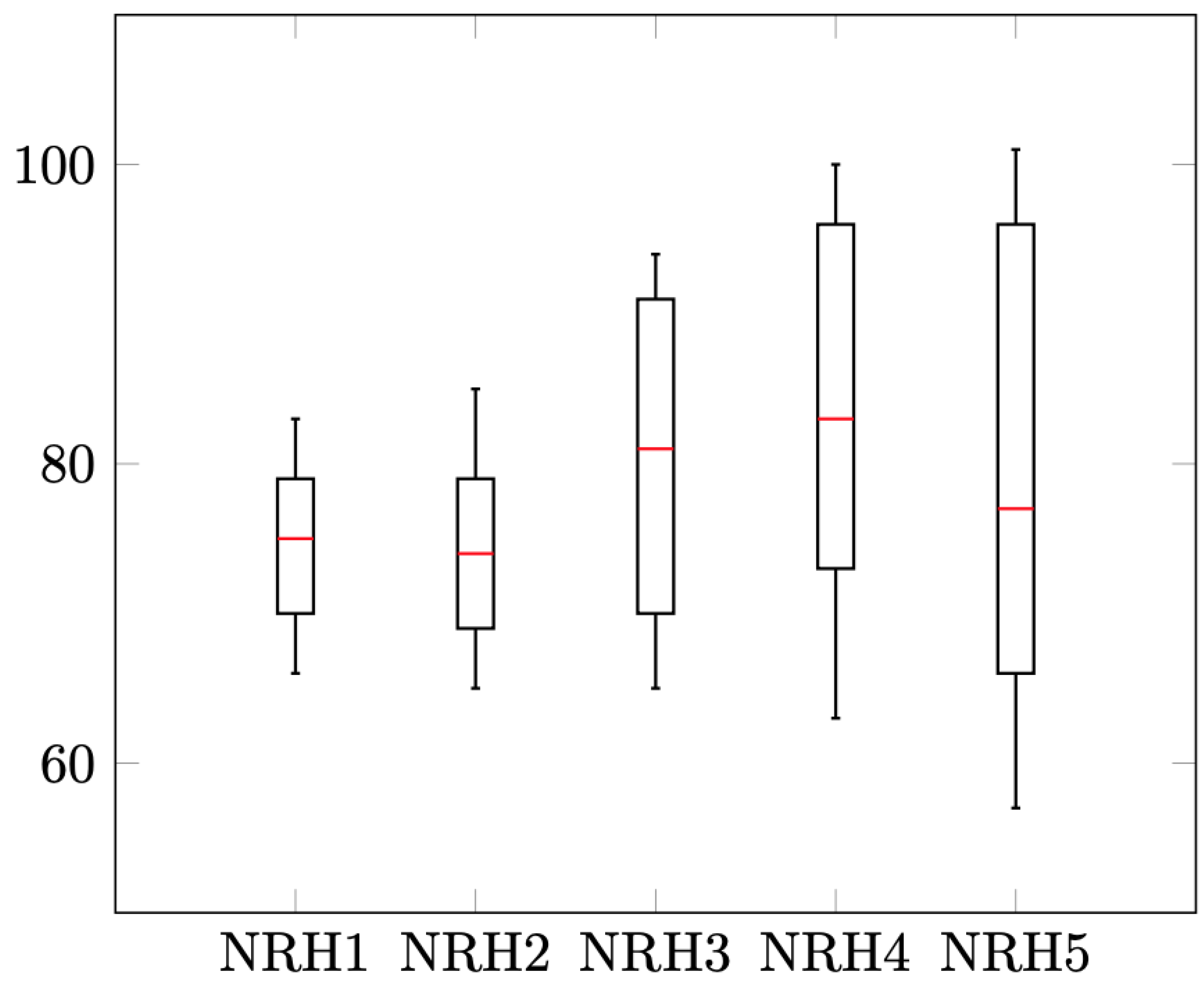
Figure 9, Figure 10, Figure 11 and Figure 12 show the results distribution for each instance, considering the minimum, maximum, median and interquartile distance for the DT algorithm version.

Some regularity can be observed in them, with a median approximately equidistant from the quartiles. The intervals between the maximum and minimum, as well as among the quartiles vary, according to the probabilistic nature of the algorithms.

8. Conclusions

In this work, we presented a framework that combines clustering and distributed parallelism to improve the metaheuristic search process. With the exception of a single instance, all of them showed improvements with regard to the best values obtained using the standalone algorithms or at least equaled them. In the experiments, 70% of the instances had the same or better RPD with the DT version than with the best of the standalone executions, achieving even more global optimums.

Removing the collaborative and clustering elements from the analysis results in a parallel execution of several algorithm instances processing the same dataset and with the same configuration, i.e., the equivalent of running the same number of experiments sequentially. We can then expect the results to be very similar to those obtained by the standalone experiments. However, this is not the case.

The results show an improvement in the RPD and statistical consistency of the DT executed algorithms. So, the key factors in any improvement are explained by the elements outside the algorithms, i.e., their collaborative work and the clustering of the search space. The obtained results reflect that the proposed architecture is more efficient when solving larger instances, making it a competitive alternative for difficult optimization problems.

From the results, we can see that although the number of nodes used is an important variable for improving the performance of a standalone algorithm, these improvements do not scale linearly, i.e., doubling the number of nodes does not necessarily double the number of best results, or halve the time required to find an optimum.

An important aspect is that the proposed approach, which is based on big data tools, makes solutions easier and cheaper, as it greatly automates the classic coding concerns associated with building distributed environments while maintaining an excellent degree of scalability. On the other hand, the clustering proved efficient in stimulating exploration of various types of neighborhoods, as the collaboration helped in exploiting those with good solutions. It should be noted that one aspect that appears to be important is that the correct selection of the algorithms to collaborate is crucial, thus making collaborations based on similar convergence rates a requisite.

The results of this work suggest research that can allow greater control and predictability of the process, such as not only clustering the initial sets of solutions, but also during the process, as the results progress.

References

- Carbas, S.; Toktas, A.; Ustun, D. Nature-Inspired Metaheuristic Algorithms for Engineering Optimization Applications, 1st ed.; Springer: Berlin/Heidelberg, Germany, 2021. [Google Scholar]
- Stegherr, H.; Heider, M.; Hähner, J. Classifying Metaheuristics: Towards a unified multi-level classification system. Nat. Comput. 2020. [Google Scholar] [CrossRef]
- Morales-Castañeda, B.; Zaldívar, D.; Cuevas, E.; Fausto, F.; Rodríguez, A. A better balance in metaheuristic algorithms: Does it exist? Swarm Evol. Comput. 2020, 54, 100671. [Google Scholar] [CrossRef]
- Hatamlou, A. Black hole: A new heuristic optimization approach for data clustering. Inf. Sci. 2013, 222, 175–184. [Google Scholar] [CrossRef]
- Jaramillo, A.; Crawford, B.; Soto, R.; Mansilla, S.; Rubio, Á.G.; Salas, J.; Olguín, E. Solving the Set Covering Problem with the Soccer League Competition Algorithm. Trends Appl. Knowl.-Based Syst. Data Sci. 2014, 9799, 884–891. [Google Scholar] [CrossRef]
- Eusuff, M.; Lansey, K.; Pasha, F. Shuffled frog-leaping algorithm: A memetic meta-heuristic for discrete optimization. Eng. Optim. 2004, 9799, 884–891. [Google Scholar] [CrossRef]
- Dhiman, G.; Kumar, V. Spotted hyena optimizer: A novel bio-inspired based metaheuristic technique for engineering applications. Adv. Eng. Softw. 2017, 114, 48–70. [Google Scholar] [CrossRef]
- García, J.; Yepes, V.; Martí, J. A Hybrid k-Means Cuckoo Search Algorithm Applied to the Counterfort Retaining Walls Problem. Mathematics 2020, 8, 555. [Google Scholar] [CrossRef]
- Cheng, S.; Liu, B.; Ting, T.; Qin, Q.; Shi, Y.; Huang, K. Survey on data science with population-based algorithms. Big Data Anal. 2016, 1, 3. [Google Scholar] [CrossRef] [Green Version]
- Harifi, S.; Khalilian, M.; Mohammadzadeh, J.; Ebrahimnejad, S. Using Metaheuristic Algorithms to Improve k-Means Clustering: A Comparative Study. Rev. D’Intell. Artif. 2020, 34, 297–305. [Google Scholar] [CrossRef]
- Olivares, R.; Muñoz, R.; Soto, R.; Crawford, B.; Cárdenas, D.; Ponce, A.; Taramasco, C. An Optimized Brain-Based Algorithm for Classifying Parkinson’s Disease. Appl. Sci. 2020, 10, 1827. [Google Scholar] [CrossRef] [Green Version]
- Hardi, M.; Zrar, A.; Tarik, R.; Abeer, A.; Nebojsa, B. A new K-means grey wolf algorithm for engineering problems. World J. Eng. 2021, 18, 630–638. [Google Scholar] [CrossRef]
- Muñoz, R.; Olivares, R.; Taramasco, C.; Villarroel, R.; Soto, R.; Barcelos, T.; Merino, E.; Alonso-Sánchez, M.F. Using Black Hole Algorithm to Improve EEG-Based Emotion Recognition. Comput. Intell. Neurosci. 2018, 2018, 3050214. [Google Scholar] [CrossRef] [PubMed]
- SaiSindhuTheja, R.; Shyama, G. An efficient metaheuristic algorithm based feature selection and recurrent neural network for DoS attack detection in cloud computing environment. Appl. Soft Comput. 2021, 100, 106997. [Google Scholar] [CrossRef]
- Bacanin, N.; Bezdan, T.; Tuba, E.; Strumberger, I.; Tuba, M. Optimizing Convolutional Neural Network Hyperparameters by Enhanced Swarm Intelligence Metaheuristics. Algorithms 2020, 13, 67. [Google Scholar] [CrossRef] [Green Version]
- Santamaría, J.; Rivero-Cejudo, M.; Martos-Fernández, M.; Roca, F. An Overview on the Latest Nature-Inspired and Metaheuristics-Based Image Registration Algorithms. Appl. Sci. 2020, 10, 1928. [Google Scholar] [CrossRef] [Green Version]
- Oliveira, G.; Coutinho, F.; Campellob, R.; Naldi, M. Improving k-means through distributed scalable metaheuristics. Neurocomputing 2017, 246, 45–57. [Google Scholar] [CrossRef]
- Zhang, P.; Yin, Z.Y.; Jin, Y.F.; Chan, T.; Gao, F.P. Intelligent modelling of clay compressibility using hybrid meta-heuristic and machine learning algorithms. Geosci. Front. 2021, 12, 441–452. [Google Scholar] [CrossRef]
- Mallick, J.; Alqadhi, S.; Talukdar, S.; AlSubih, M.; Ahmed, M.; Abad, R.; Ben, N.; Abutayeh, S. Risk Assessment of Resources Exposed to Rainfall Induced Landslide with the Development of GIS and RS Based Ensemble Metaheuristic Machine Learning Algorithms. Sustainability 2021, 13, 457. [Google Scholar] [CrossRef]
- Nayak, J.; Naik, B.; Byomakesha, P.; Pelusi, D. Optimal Fuzzy Cluster Partitioning by Crow Search Meta-Heuristic for Biomedical Data Analysis. Int. J. Appl. Metaheuristic Comput. 2021, 12, 49–66. [Google Scholar] [CrossRef]
- Memeti, S.; Pllana, S.; Binotto, A.; Kołodziej, J.; Brandic, I. Using meta-heuristics and machine learning for software optimization of parallel computing systems: A systematic literature review. Computing 2019, 101, 893–936. [Google Scholar] [CrossRef] [Green Version]
- Talbi, E.G. Machine Learning into Metaheuristics: A Survey and Taxonomy. ACM Comput. Surv. 2022, 54, 1–32. [Google Scholar] [CrossRef]
- Hassan, A.; Pillay, N. Hybrid metaheuristics: An automated approach. Expert Syst. Appl. 2019, 130, 132–144. [Google Scholar] [CrossRef]
- Oliva, D.; Hinojosa, S. Applications of Hybrid Metaheuristic Algorithms for Image Processing, 1st ed.; Springer: Berlin/Heidelberg, Germany, 2020. [Google Scholar]
- Pellerin, R.; Perrier, N.; Berthaut, F. A survey of hybrid metaheuristics for the resource-constrained project scheduling problem. Eur. J. Oper. Res. 2020, 280, 395–416. [Google Scholar] [CrossRef]
- Shukla, A.K.; Singh, P.; Vardhan, M. Gene selection for cancer types classification using novel hybrid metaheuristics approach. Swarm Evol. Comput. 2020, 54, 100661. [Google Scholar] [CrossRef]
- Fakhrzad, M.B.; Goodarzian, F.; Golmohammadi, A.M. Addressing a fixed charge transportation problem with multi-route and different capacities by novel hybrid meta-heuristics. J. Ind. Syst. Eng. 2019, 12, 167–184. [Google Scholar]
- Ikeda, S.; Nagai, T. A novel optimization method combining metaheuristics and machine learning for daily optimal operations in building energy and storage systems. Appl. Energy 2021, 289, 116716. [Google Scholar] [CrossRef]
- Hijazi, N.; Faris, H.; Aljarah, I. A parallel metaheuristic approach for ensemble feature selection based on multi-core architectures. Expert Syst. Appl. 2021, 182, 115290. [Google Scholar] [CrossRef]
- Arkhipov, D.; Wu, D.; Wu, T.; Regan, A. A Parallel Genetic Algorithm Framework for Transportation Planning and Logistics Management. Intell. Logist. Based Big Data 2020, 8, 106506–106515. [Google Scholar] [CrossRef]
- Khanduja, N.; Bhushan, B. Recent Advances and Application of Metaheuristic Algorithms: A Survey (2014–2020). Metaheuristic Evol. Comput. Algorithms Appl. 2020, 916, 207–228. [Google Scholar] [CrossRef]
- Mouton, J.; Ferreira, M.; Helberg, A. A comparison of clustering algorithms for automatic modulation classification. Expert Syst. Appl. 2020, 151, 113–317. [Google Scholar] [CrossRef]
- Moosavian, N.; Kasaee, B. Algorithm AS 136: A K-Means Clustering Algorithm. J. R. Stat. Soc. Ser. C 2014, 17, 14–24. [Google Scholar]
- Gowda, K.C.; Krishna, G. Agglomerative clustering using the concept of mutual nearest neighbourhood. Pattern Recognit. 1978, 10, 105–112. [Google Scholar] [CrossRef]
- Sridevi, K.; Prakasha, S. Comparative Study on Various Clustering Algorithms Review. In Proceedings of the 5th International Conference on Intelligent Computing and Control Systems (ICICCS), Madurai, India, 6–8 May 2021; Volume 151, pp. 153–158. [Google Scholar] [CrossRef]
- Zhou, H.; Gao, J. Automatic Method for Determining Cluster Number Based on Silhouette Coefficient. Adv. Mater. Res. 2014, 951, 227–230. [Google Scholar] [CrossRef]
- Karp, R. Reducibility Among Combinatorial Problems. 1972. Available online: https://cs.stanford.edu/people/trevisan/cs172-04/karp.pdf (accessed on 13 January 2021).
- Daskin, M. Application of an expected covering model to emergency medical service system design. Decis. Sci. 1982, 13, 416–439. [Google Scholar] [CrossRef]
- Chen, L.; Yuan, D. Solving a minimum-power covering problem with overlap constraint for cellular network design. Eur. J. Oper. Res. 2010, 203, 714–723. [Google Scholar] [CrossRef] [Green Version]
- ReVelle, C.; Toregas, C.; Falkson, L. Applications of the Location Set-covering Problem. Geogr. Anal. 1976, 8, 65–76. [Google Scholar] [CrossRef]
- Moosavian, N.; Kasaee, B. Soccer league competition algorithm: A novel meta-heuristic algorithm for optimal design of water distribution networks. Swarm Evol. Comput. 2014, 17, 14–24. [Google Scholar] [CrossRef]
- Beasley, J. OR-Library,1990. Available online: http://people.brunel.ac.uk/~mastjjb/jeb/info.html (accessed on 13 January 2021).
- Grossman, T.; Wool, A. Computational experience with approximation algorithms for the set covering problem. Eur. J. Oper. Res. 1997, 101, 81–92. [Google Scholar] [CrossRef]
- Derrac, J.; García, S.; Molina, D.; Herrera, F. A practical tutorial on the use of nonparametric statistical tests as a methodology for comparing evolutionary and swarm intelligence algorithms. Swarm Evol. Comput. 2011, 1, 3–18. [Google Scholar] [CrossRef]
- García, S.; Molina, D.; Lozano, M.; Herrera, F. A study on the use of non-parametric tests for analyzing the evolutionary algorithms behaviour: A case study onthecec2005 special session onreal parameter optimization. J. Heuristics 2008, 15, 617–644. [Google Scholar] [CrossRef]
- Lanza-Gutierrez, J.; Gómez-Pulido, J. Assuming multiobjective metaheuristics to solve a three-objective optimization problem for relay node deployment in wireless sensor networks. Appl. Soft Comput. 2015, 30, 675–687. [Google Scholar] [CrossRef]