Building 2D Model of Compound Eye Vision for Machine Learning

Abstract

This paper presents a two-dimensional mathematical model of compound eye vision. Such a model is useful for solving navigation issues for autonomous mobile robots on the ground plane. The model is inspired by the insect compound eye that consists of ommatidia, which are tiny independent photoreception units, each of which combines a cornea, lens, and rhabdom. The model describes the planar binocular compound eye vision, focusing on measuring distance and azimuth to a circular feature with an arbitrary size. The model provides a necessary and sufficient condition for the visibility of a circular feature by each ommatidium. On this basis, an algorithm is built for generating a training data set to create two deep neural networks (DNN): the first detects the distance, and the second detects the azimuth to a circular feature. The hyperparameter tuning and the configurations of both networks are described. Experimental results showed that the proposed method could effectively and accurately detect the distance and azimuth to objects.

1. Introduction

Robotics is a rapidly developing industrial area. The modern classification of robots is based on the environment in which the robot operates and its functionality. One of the most important functions is the ability of the robot to move in the operating environment. Robots capable of movement are classified as mobile. Robots that do not have functionality for movement are classified as fixed. An example of a fixed robot is a robot manipulator, widely used in assembly production. Such a robot operates in an environment adapted for its functioning. In contrast, mobile robots have to operate in boundless spaces in a changing environment under conditions that are not known in advance [1]. Mobile robots are divided into two subclasses: autonomous and non-autonomous. The non-autonomous mobile robot rely on operator control. The robot transmits the signals coming from the sensors to the operator via wireless channels. The information obtained allows the operator to detect hazards, obstacles, and distances to objects. The operator decides on the robot’s further actions and sends him the appropriate commands. The autonomous robot has no connection with the operator and must make decisions about further actions on its own.

A crucial element of mobile robots is the use of sensors. One of the most important sensors for autonomous mobile robots is the distance sensor, which detects the distance from the robot to the object. Using two distance sensors or rotating one sensor, the robot can detect the azimuth of an object relative to the direction of its movement. The distance sensor is classified as active or passive [2]. The active distance sensor emits a signal of a certain nature and detects its reflection from the object. The time difference between the sent and received signals allows the robot to measure the distance to the object. Ultrasonic and laser distance sensors work in this way [3]. The infrared distance sensor works on a different principle: the light intensity decreases in proportion to the square of the distance to the object. This ratio is used to measure the approximate distance between the robot and the object. The laser triangulation [4] is the third way to calculate the distance to an object. Active distance sensors have two common disadvantages: first, they consume additional energy to generate rays, and second, a robot with active sensors can be detected by an external observer, which is not always permissible. The passive sensor does not emit any signals. It uses only the light reflected by the object. A well-known example of passive sensors is a digital camera [4]. The distance between the object and an observer can be calculated by using visual information gained from a pair of images taken by two cameras, which is known as stereo image [5]. A stereo camera requires sophisticated controls, including panning, tilting, zooming, focusing on, and tracking a moving object [6]. For this reason, the use of stereo cameras in fully autonomous robots is difficult.

Video sensors inspired by compound eyes of insects are promising alternatives to digital cameras [7]. Such video sensors have no moving parts and do not require any control. The insect vision has the following three basic configurations: apposition, superposition, and neural superposition compound eyes [8]. Each configuration has its advantages and disadvantages. Apposition compound eyes consist of hundreds up to tens of thousands of microlens receptor units, called ommatidia, arranged on a curved surface. Each ommatidium consists of a microlens (facet lens) and a small group of rhabdomere (photoreceptor) bundles, called the rhabdom. The pigments form opaque walls between adjacent ommatidia to avoid the light focused by one microlens on the receptor of the adjacent channel [7]. There are no moving or dynamically transforming parts in the apposition compound eye, and it does not need to be controlled by the nervous system. The spatial acuity of the apposition compound eye is determined by the interommatidial angle $\Delta \varphi =D/R$, where D is the diameter of the facet lens and R is the local radius of curvature of the eye [9]. The superposition eye gathers light beams from adjacent ommatidia. This effectively enhances the photosensitivity, but reduces the effective acuity due to the blurring effect. In the neural superposition eye, one rhabdomere in several adjacent ommatidia shares an overlapped field of view with the other. A large amount of overlap can lead to an increase in the signal-to-noise ratio. Therefore, overlapping fields provide a better resolution of motion than that implied by the distance between the facets of the compound eye, a phenomenon known as hyperacuity [10].

The apposition vision configuration is the most promising for robotics because of its simplicity. In recent years, great progress has been achieved in the design of video sensors inspired by the artificial composite eyes of this structure [11]. The first artificial compound eye, constructed in 1991, had a weight of 1 kg, a diameter of 23 cm, and consisted of 118 artificial ommatidia with a facet diameter of 6 mm [12,13]. The artificial compound eye, created in 2013, has a weight of 1.75 g, a diameter of 12.8 mm, and consists of 630 artificial ommatidia with a facet diameter of 172 μm [14]. Modern technologies allow creating the curved microlens arrays with a diameter of 500 μm, consisting of microlens with a diameter of 20 μm [15].

In this paper, we present a mathematical model of the planar binocular compound eye vision, focusing on measuring distance and azimuth to a circular feature with an arbitrary size. The model provides a necessary and sufficient condition for the visibility of a circular feature by each ommatidium. On this basis, an algorithm is built for generating a training data set. We used the generated data set to create two ANNs: the first detects the distance, and the second detects the azimuth to a circular feature. The rest of the paper is organized as follows. Section 2 provides a review of known methods for measuring the distance and azimuth to an object using passive optical sensors. In Section 3, we present a mathematical model of the planar compound eye vision. Section 4 is devoted to the issues of generating a training set based on the presented model of planar compound eye vision. Section 5 describes two deep neural networks that calculate the distance and azimuth to a circular feature based on data yielded by a planar binocular compound eye system. In Section 6, we describe the computational experiments with the developed neural networks. Section 7 discusses the issues related to the main contribution of this article, the advantages and disadvantages of the proposed approach, possible applications, and some other aspects of the presented model. Section 8 summarizes the obtained results and outlines the directions of future research.

2. Related Work

This section presents an overview of works devoted to mathematical models and methods for measuring distance and azimuth to an object based on passive optical sensors. One of the simplest methods is bearing-based distance measurement [16] (see Figure 1).

This method calculates distance $d_{object}$ to an object from known height $h_{camera}$ of the observing camera, angle $\phi$ of the camera tilt, and height $h_{object}$ of the object:

$$(h_{camera}-h_{object})tan\phi .$$

(1)

This simple model is only valid when $h_{camera}>h_{object}$ and $\phi <\frac{\pi }{2}$. In addition, we need to know height $h_{object}$ of the object, which is not always feasible in practice. The measurement error as a function of $\Delta \phi$ can be estimated as follows:

$$d_{error}(\Delta \phi )= \left|(tan(\phi +\Delta \phi )-tan\left(\phi \right))·(h_{camera}-h_{object})\right|.$$

(2)

It is obvious from this equation that the error is rising exponentially for positive $\Delta \phi$ with fixed $h_{camera}$ and $h_{object}$. Thus, this method is not applicable when the height of the camera is comparable to the height of the object.

In [17,18,19], a monocular vision model is proposed for determining the 3D position of circular and spherical features. This model uses a 2D image representing a perspective projection of a feature and the effective focal length of the camera to find the feature’s location, with respect to the camera frame. The described method can be generalized for 3D quadratic features, such as ellipsoid, paraboloid, hyperboloid, and cylindroid, but not for features of arbitrary shape. In addition, this method has a relatively high computational complexity and cannot provide sufficient accuracy in measuring the distance to the visible object.

The next method for determining the distance to a visible object is based on using two video cameras having the same specifications, which are conjugated in a certain way to generate a stereo image in the form of two 2D images [20,21,22,23,24]. This method is based on epipolar geometry [25,26]. The sense of the method is as follows. Let $C_l$ be the center of the left video camera, $C_r$ be the center of the right video camera, and P be the point to detect distance. The epipolar plane is the plane determined by three points $(C_l,C_r,P)$. In this model, the image sensor matrices are located in the same plane perpendicular to the epipolar plane. Let $P_l$ and $P_r$ be the images of point P in the left and right image sensor matrices, accordingly. Denote by $u_l$, $u_r$ the distances from the points $P_l$, $P_r$ to the centers of the corresponding image sensor matrices. Then, distance d between point P and the center of the stereo camera system can be calculated as follows:

$$d=\frac{bf}{u_l+u_r},$$

(3)

where b is the distance between video cameras, and f is the focal length. To find the point of interest in the left image, we must perform the object segmentation procedure [26]. This gives us point $P_l$. To find the corresponding point $P_r$ on the right image, we must perform the stereo matching procedure [27] for both images. First of all, we must perform a careful camera calibration process [28]. All of this makes it difficult to use this method for autonomous mobile robots. In addition, this technique cannot provide high measurement accuracy.

Another passive method to measure the distance to an object is to use a plenoptic camera [29]. A plenoptic or light-field camera acts like a micro camera array that records not only the light intensity but a combination of light intensity and the direction of incident light rays. The distance estimation is based on disparities observed in neighboring microlens images, similar to stereo camera approaches. The plenoptic camera can give 3D information for every point of the scene with one camera, one main lens, and a microlens array placed directly in front of the image sensor. The price that has to be paid for these additional features is a significant reduction in the effective image resolution [30]. A geometric optical model to measure the distance to an object using a light field image is proposed in [31]. The distance $d_{out}$ between main lens and an object can be calculated by the following equation:

$$d_{out}=\frac{D}{2tan\phi }+\sqrt{R^2+D^2/4}-R+T/2,$$

(4)

where R represents the radius of curvature of main lens; T represents the central thickness of main lens and D is the pupil diameter of main lens. The angle $\phi$ is calculated by

$$\phi =arcsin\left(n_{1}sin\psi \right)-arcsin\left(\frac{D}{2R}\right),$$

(5)

where $n_1$ is the refractive index of the main lens; $\psi$ is the included angle between the normal and the refractive light rays in the main lens. The refractive angle $\psi$ can be calculated by the following known camera parameters: the focal length $f_x$ of microlens array, the distance $d_{in}$ between the microlens array and main lens, and the length H of corresponding light field [31]. The described method also requires a complex camera calibration process [30], does not provide a high measurement accuracy at long distances [32], and it is poorly suited for autonomous mobile robots.

By reviewing the related papers, one notices a lack of work devoted to mathematical models of distance measurement using artificial binocular compound eye vision systems. At the same time, the progress made in manufacturing artificial compound eyes and their unique features make this issue urgent.

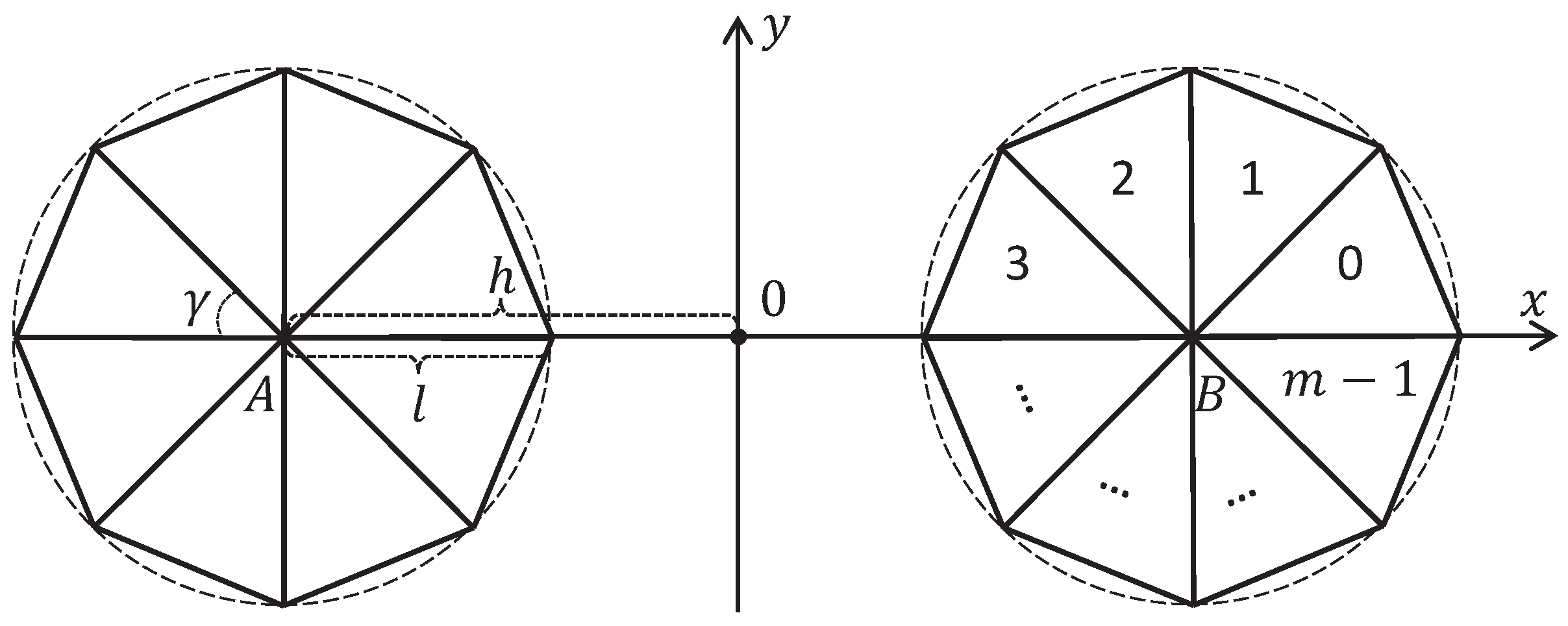
3. Two-Dimensional Model of Compound Eye Vision

The 2D model of binocular compound eye vision includes two circular compound eyes located symmetrically relative to the y-axis, the centers A and B of which lie on the x-axis (see Figure 2).

The distance from the origin to the center of each eye is equal to h. The composite eye consists of m ommatidia, represented as equal-sized isosceles triangles. The legs have the length l, and the base has the length s. The angle between the legs is equal to $\gamma$. It is obvious that

$$\gamma =\frac{2\pi }{m}.$$

(6)

In this model, we assume that $h>l,$ and $m⩾4$. Taking into account (6), it follows

$$\gamma ⩽\frac{\pi }{2}.$$

(7)

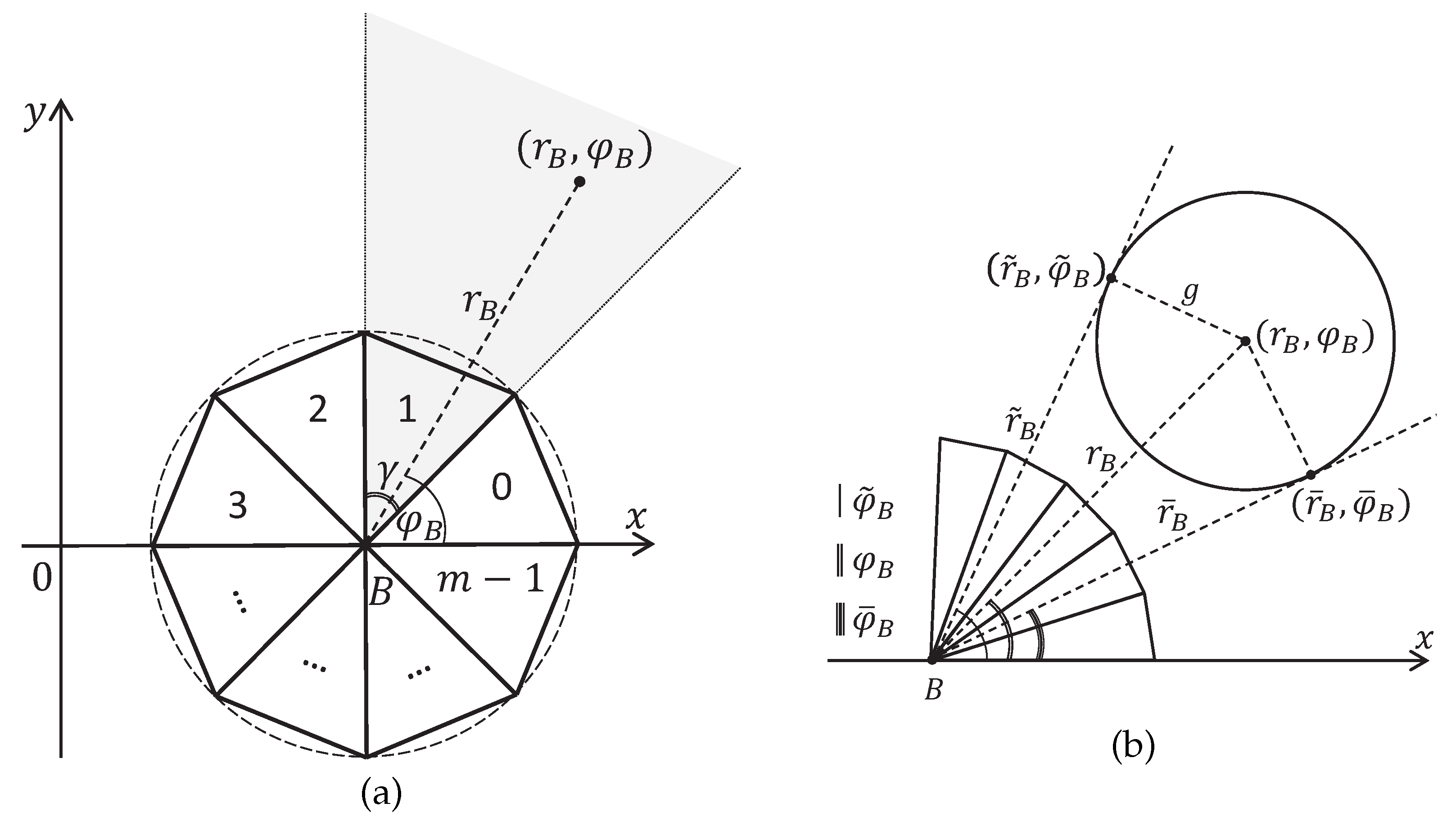
Let us number the ommatidia counterclockwise from 0 to $m-1$, starting with the ommatidium, which lies on the x-axis (see the right eye in Figure 2). In the model, the ommatidium field of view is defined as a solid angle bounded by its legs. In Figure 3a, the gray solid angle depicts the field of view of the ommatidium with number 1. If a point lies on the bound between adjacent ommatidia, then it is visible only for the ommatidium with the larger number. Thus, the fields of view of different ommatidia do not intersect, and their unions form a solid angle of ${360}^{\circ }$.

Let us build a ray tracing model. Consider the polar coordinate system $(r_B,{\phi }_B)$ with the origin in the point B and the angle measured from the x-axis. The following Proposition 1 gives an equation to calculate the number of ommatidia, which observes the point with given polar coordinates (see Figure 3a).

Proposition 1.

Let the point $(r_B,{\phi }_B)$ be given in polar coordinates with center B. The number k of the ommatidium, to whose field of view the point $(r_B,{\phi }_B)$ belongs, is determined by the equation

$$k=⌊\frac{m}{2\pi }{\phi }_B⌋.$$

(8)

Proof. 

It follows from Equation (6) that the angle ${\phi }_B$ must satisfy the system of inequalities

$$\left\{\begin{array}{c}{\phi }_B⩾\frac{2\pi }{m}k;\hfill \\ {\phi }_B<\frac{2\pi }{m}(k+1).\hfill \end{array}\right.$$

(9)

Convert this system to the form

$$\left\{\begin{array}{c}k⩽\frac{m}{2\pi }{\phi }_B;\hfill \\ k>\frac{m}{2\pi }{\phi }_B-1.\hfill \end{array}\right.$$

(10)

By the definition of the greatest integer less than or equal to $\frac{m}{2\pi }{\phi }_B$, it follows (8).   □

The next proposition extends Proposition 1 for the case of circular features (see Figure 3b).

Proposition 2.

Let a circular feature with radius g and center $(r_B,{\phi }_B)$ in polar coordinates with center B be given. This circular feature or part of it belongs to the field of view of the ommatidium with the number k if and only if

$$⌊\frac{m}{2\pi }\left({\phi }_B-arcsin\left(\frac{g}{r_B}\right)\right)⌋⩽k⩽⌊\frac{m}{2\pi }\left({\phi }_B+arcsin\left(\frac{g}{r_B}\right)\right)⌋.$$

(11)

Proof. 

Consider the tangents to the circle at the points $\left({\overline{r}}_B,{\overline{\phi }}_B\right)$ and $\left({\tilde{r}}_B,{\tilde{\phi }}_B\right)$ passing through the point B in Figure 3b. We have

$${\overline{\phi }}_B={\phi }_B-arcsin\frac{g}{r_B};{\tilde{\phi }}_B={\phi }_B+arcsin\frac{g}{r_B}.$$

(12)

Taking into account Proposition 1, it follows (11).    □

Definition 1.

In the context of the model under consideration, an object is invisible to the compound eye if and only if it lies in the field of view of only one ommatidium.

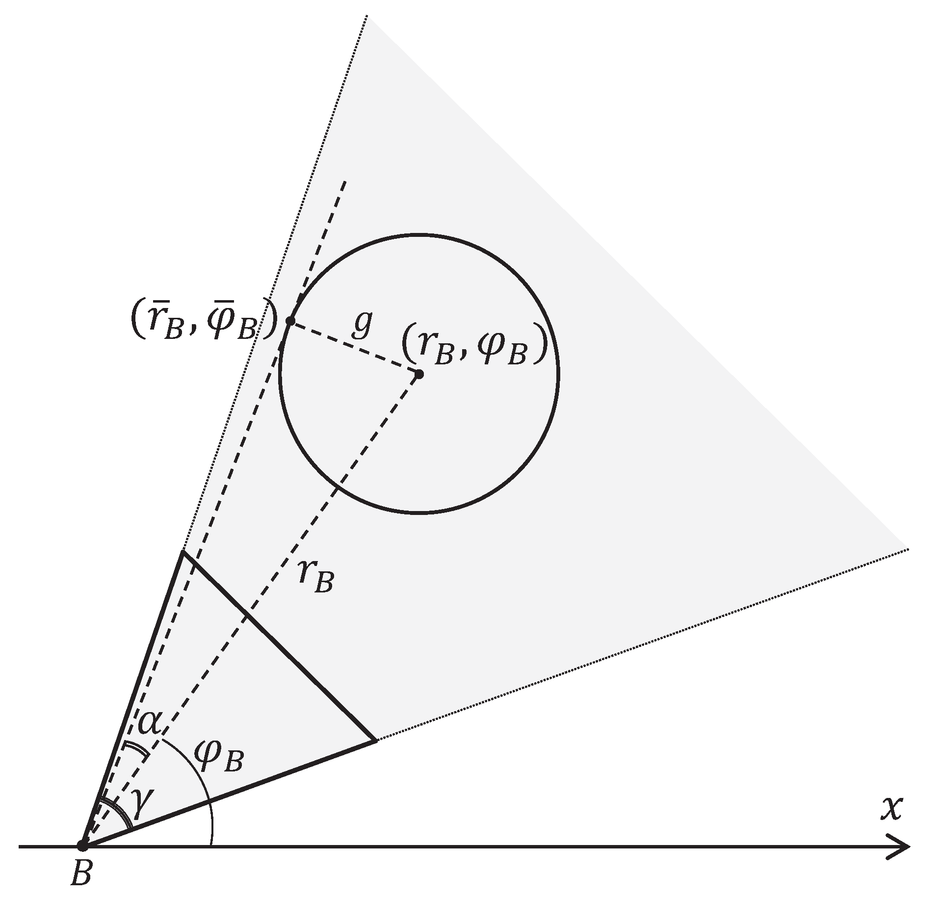
The following proposition gives us a sufficient condition for the visibility of the circular feature.

Proposition 3.

Let a circular feature with radius g and center $(r_B,{\phi }_B)$ in polar coordinates with center B be given. Let γ be the view field angle of an ommatidium. The inequality

$$g>r_{B}sin\frac{\gamma }{2}$$

(13)

is a sufficient condition for the visibility of the circular feature.

Proof. 

Let us assume the opposite: the circular feature with radius g and center $(r_B,{\phi }_B)$ is invisible, and inequality (13) holds. Consider the tangent to the circle at the point $\left({\overline{r}}_B,{\overline{\phi }}_B\right)$ passing through the point B in Figure 4.

Let $\alpha$ be the angle between this tangent and the ray from the point B to the point $(r_B,{\phi }_B)$. Taking into account Definition 1, inequality (7) and inequality (13), we obtain

$$g=r_{B}sin\alpha ⩽r_{B}sin\frac{\gamma }{2}<g.$$

(14)

Thus we have a contradiction.    □

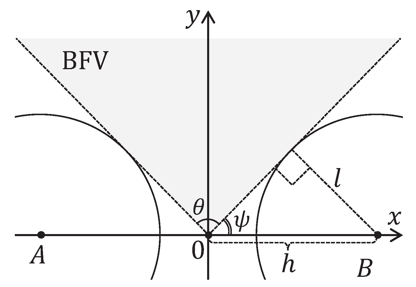
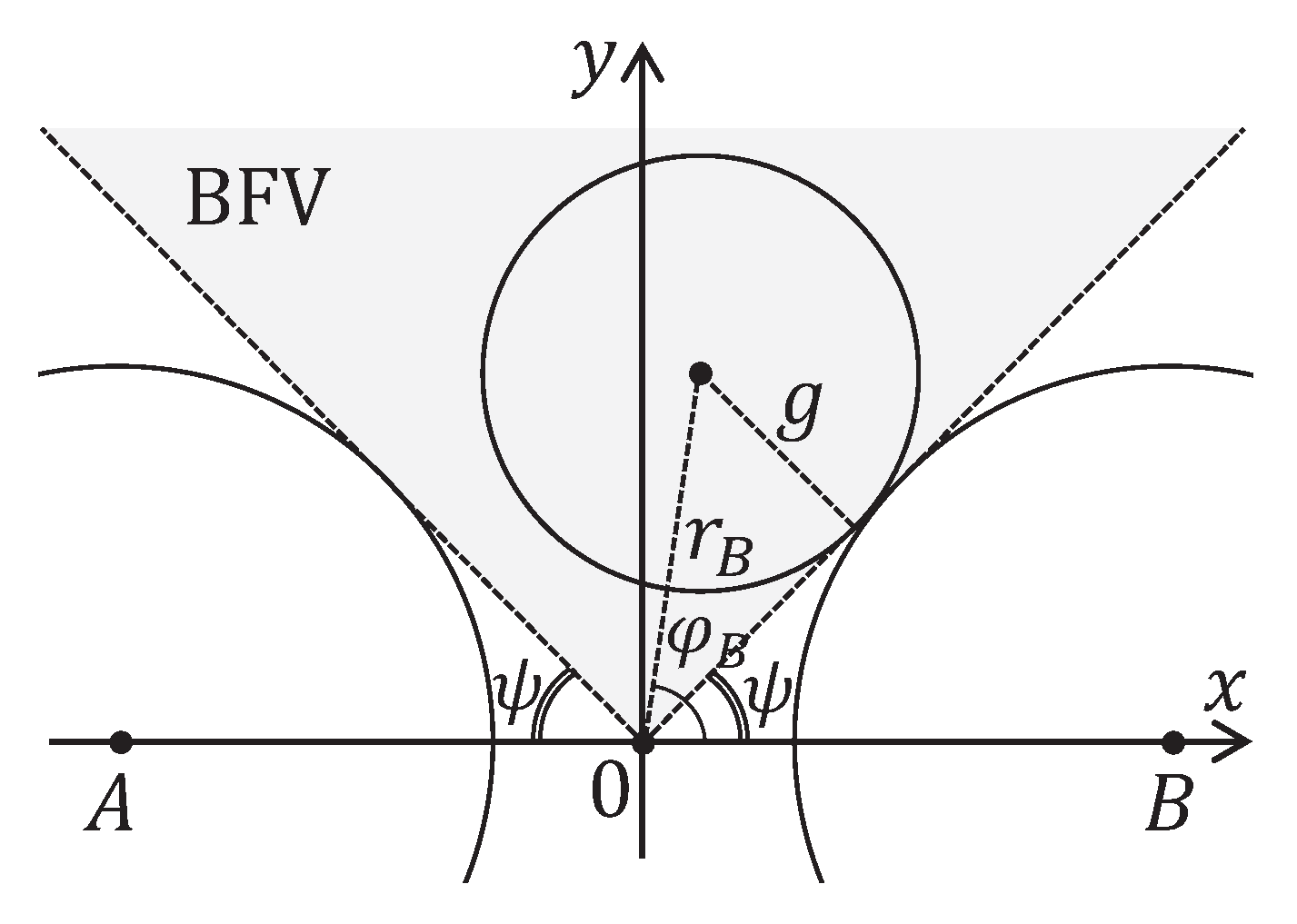
Definition 2.

In the context of the model under consideration, the binocular field of view (BFV) is the solid angle θ between the tangents to the compound eye circles drawn from the origin in the direction of the positive y-axis (see Figure 5).

BFV is uniquely determined by the angle $\psi$ between the right tangent and the x axis. Obviously,

$$\psi =arcsin\frac{l}{h}.$$

(15)

It follows

$$\theta =\pi -2arcsin\frac{l}{h}.$$

(16)

BFV has the following three important properties.

Property 1.

Any object lying in BFV does not cross the compound eyes.

Property 2.

Any object lying in the BFV is entirely visible to both compound eyes.

Property 3.

Any circular feature lying in BFV is invisible to all ommatidia located in the negative region of the y-axis.

The following proposition gives us a necessary and sufficient condition for a circular feature to lie entirely in BFV.

Proposition 4.

Let a circular feature with the radius g and the center $(r,\phi )$ in the polar coordinates centered at the origin be given ($0⩽\phi <2\pi$). This circular feature lies entirely inside the BFV defined by the angle ψ if and only if

$$\psi +arcsin\frac{g}{r}⩽\phi ⩽\pi -\psi -arcsin\frac{g}{r}.$$

(17)

Proof. 

Consider a circular feature with the radius g and the center $(r,\phi )$ that touches the right bound of BFV in the Figure 6.

Using right triangle properties, we have

$$g=rsin(\phi -\psi ).$$

(18)

It follows

$$\phi =\psi +arcsin\frac{g}{r}.$$

(19)

Hence, a circular feature with the radius g and the center $(r,\phi )$ lies to the left of the right BFV bound if and only if

$$\phi ⩾\psi +arcsin\frac{g}{r}.$$

(20)

In the same way, we obtain that a circular feature with the radius g and the center $(r,\phi )$ lies to the right of the left BFV bound if and only if

$$\phi ⩽\pi -\psi -arcsin\frac{g}{r}.$$

(21)

   □

Below, in the algorithm generating the training data set (see Section 4), we will need equations that convert the polar coordinates $(r,\phi )$ centered at the origin to the polar coordinates $(r_A,{\phi }_A)$ centered at the point $A=(0,-h)$ for the left compound eye, and to the polar coordinates $(r_B,{\phi }_B)$ centered at the point $B=(0,h)$ for the right compound eye. The following proposition provides us with such equations.

Proposition 5.

Let $0⩽\phi ⩽\pi$, $0<h$, $0<r$ be given. For the polar coordinates $(r,\phi )$ centered at the origin, the following equations convert them to the polar coordinates $(r_B,{\phi }_B)$ centered at the point $B=(0,h)$, and to the polar coordinates $(r_A,{\phi }_A)$ centered at the point $A=(0,-h)$:

$$r_B=\sqrt{h^2+r^2-2hrcos\phi };$$

(22)

$${\phi }_B=\pi -arccos\frac{h-rcos\phi }{\sqrt{h^2+r^2-2hrcos\phi }};$$

(23)

$$r_A=\sqrt{h^2+r^2+2hrcos\phi };$$

(24)

$${\phi }_A=arccos\frac{h+rcos\phi }{\sqrt{h^2+r^2+2hrcos\phi }}.$$

(25)

Proof. 

Take a look at Figure 7b.

By the law of cosines, we have:

$$r_B=\sqrt{h^2+r^2-2hrcos\phi };$$

(26)

$$\beta =arccos\frac{h^2+{r_B}^2-r^2}{2h{r}_B}.$$

(27)

Taking into account that $\beta =\pi -{\phi }_B$, it follows

$${\phi }_B=\pi -arccos\frac{h-rcos\phi }{\sqrt{h^2+r^2-2hrcos\phi }}.$$

(28)

In the same way, in the context of Figure 7a, we can obtain Equations (24) and  (25).    □

4. Algorithm for Generating Training Data Set

Based on the proposed 2D model of binocular compound eye vision, we developed Algorithm 1 for generating annotated data sets, for training artificial neural networks capable of determining the distance and azimuth to the observed objects. The data set $\mathcal{M}\subset {\mathbb{R}}^2\times {\{0,1\}}^{m/2}\times {\{0,1\}}^{m/2}$ consists of elements of the form $(r,\phi ,{\Omega }_A,{\Omega }_B)$. Each element corresponds to one observed circular feature with the following four parameters. The pair $(r,\phi )$ determines the polar coordinates of the circle feature center. The parameter ${\Omega }_A$ is the bit map with the length of $m/2$ produced by the left compound eye: ${\Omega }_A\left[i\right]=1$ if and only if the ith ommatidium of left eye observes the circular feature ($i=0,\dots ,m/2-1$). The parameter ${\Omega }_B$ is the bit map with the same length of $m/2$ produced by the right compound eye: ${\Omega }_B\left[j\right]=1$ if and only if the jth ommatidium of right eye observes the circular feature ($j=0,\dots ,m/2-1$).

Algorithm 1 Generating a training data set

1: input $h,l,m,n,r_{min},r_{max},g_{max}$; 2: $\gamma :=2\pi /m$; 3: $\psi :=arcsin(l/h)$; 4: $\mathcal{M}:=\varnothing$; 5: for  $i=1\dots n$  do 6:     repeat 7:         $r:=rnd(r_{min},r_{max})$; 8:         $g_{min}:=rsin(\gamma /2);$ 9:         if $g_{min}>g_{max}$ then continue; 10:         $g:=rnd(g_{min},g_{max})$; 11:         if $g>r$ then continue; 12:         $\phi :=rnd(\psi +arcsin(g/r),\pi -\psi -arcsin(g/r\left)\right)$; 13:         $r_B:=\sqrt{h^2+r^2-2hrcos\phi }$; ${\phi }_B:=\pi -arccos\frac{h-rcos\phi }{\sqrt{h^2+r^2-2hrcos\phi }}$; 14:         $L_B:=⌊\frac{m}{2\pi }\left({\phi }_B-arcsin\left(\frac{g}{r_B}\right)\right)⌋$; $R_B:=⌊\frac{m}{2\pi }\left({\phi }_B+arcsin\left(\frac{g}{r_B}\right)\right)⌋$; 15:         $r_A:=\sqrt{h^2+r^2+2hrcos\phi }$; ${\phi }_A:=arccos\frac{h+rcos\phi }{\sqrt{h^2+r^2+2hrcos\phi }}$; 16:         $L_A:=⌊\frac{m}{2\pi }\left({\phi }_A-arcsin\left(\frac{g}{r_A}\right)\right)⌋$; $R_A:=⌊\frac{m}{2\pi }\left({\phi }_A+arcsin\left(\frac{g}{r_A}\right)\right)⌋$; 17:         for $j=0\dots m/2-1$ do 18:            if $L_B⩽j⩽R_B$ then 19:                ${\Omega }_B\left[j\right]:=1$; 20:            else 21:                ${\Omega }_B\left[j\right]:=0$; 22:            end if; 23:            if $L_A⩽j⩽R_A$ then 24:                ${\Omega }_A\left[j\right]:=1$; 25:            else 26:                ${\Omega }_A\left[j\right]:=0$; 27:            end if; 28:         end for; 29:     until $(r,\phi ,{\Omega }_A,{\Omega }_B)\in \mathcal{M}$; 30:     $\mathcal{M}:=\mathcal{M}\cup \left\{(r,\phi ,{\Omega }_A,{\Omega }_B)\right\}$; 31: end for.

Let us make brief comments on the steps of Algorithm 1. Step 1 performs the input of the algorithm parameters:

h: the distance from the origin to the centers of compound eyes (see Figure 2);

• l: the radius of compound eye;
• m: the number of ommatidia in compound eye;
• n: the number of elements in the training data set;
• $r_{min}$: the minimum distance from the origin to the center of circular feature;
• $r_{max}$: the maximum distance from the origin to the center of circular feature;
• $g_{max}$: the maximum radius of circular feature.

Step 2 calculates the angle $\gamma$ of the ommatidium field of view according to Equation (6). In Step 3, the angle $\psi$ of the binocular field of view is calculated using Equation (15). In Step 4, the set $\mathcal{M}$ is initially defined as an empty set. Steps 5–31 implement a for loop that inserts n elements into $\mathcal{M}$. The repeat/until loop (Steps 6–29) generates one new element of the training data set. Step 7 generates the distance r from the origin to the center of circular feature using the rnd function, which calculates a random real number from the interval $[r_{min},r_{max}]$. Step 8 calculates the minimum radius of circular feature by inequality (13), which provides a sufficient condition for its visibility. Step 9 checks the condition $g_{min}>g_{max}$. If this condition is true, then it forces the repeat/until loop to begin the next iteration. Step 10 calculates the radius g of circular feature as a random real number from the interval $[g_{min},g_{max}]$. Step 11 checks the condition $g>r$. If this condition is true, then it forces the repeat/until loop to begin the next iteration. Step 12 randomly generates the angle $\phi$ so that the circular feature of the radius g and the center $(r,\phi )$ in polar coordinates lies entirely inside the binocular field of view (see Proposition 4). Step 13 converts polar coordinates $(r,\phi )$ to polar coordinates $(r_B,{\phi }_B)$ using Equations (22) and (23). Based on Proposition 2, Step 14 determines, for the right compound eye, the interval $[L_B,R_B]$, which includes the numbers of the ommatidia that observe the circular feature. In the same way, Steps 15, 16 determine the interval $[L_A,R_A]$, which includes the numbers of the ommatidia that observe the circular feature in the case of the left compound eye. Using the obtained data, Steps 17–28 generate the new element $({\Omega }_A,{\Omega }_B,r,\phi )$ to include in the training data set. If the obtained element does not have a duplicate in $\mathcal{M}$, it is added to the training data set in Step 30.

Let us estimate the computational complexity of Algorithm 1. We assume that the assignment operator, all arithmetic operations, and all comparison operations take one time unit. Let the rnd function be calculated by the Lehmer pseudo-random number generator [33] using the following equation:

$$x_{k+1}=a·x_{k}modm,$$

(29)

where the modulus m is a prime number. The function $rnd(v_{min},v_{max})$ is defined as follows:

$$rnd(v_{min},v_{max})=v_{min}+\left(x_{k+1}mod(v_{max}-v_{min})\right).$$

(30)

Then we can assume that the rnd function takes 5 time units. We also assume that the square root and all trigonometric functions are calculated using the first four terms of the Taylor series:

$$f\left(x\right)=f\left(a\right)+\frac{f^{\prime }\left(a\right)}{1!}(x-a)+\frac{f^{″}\left(a\right)}{2!}{(x-a)}^2+\frac{f^{‴}\left(a\right)}{3!}{(x-a)}^3.$$

(31)

In this case, the calculation of one function will take 17 time units. The

Table 1. Cost of operations and functions.

Term	Type	Cost
$+,-,\times ,/,\lfloor \rfloor ,mod$	Arithmetic operations	1
$>,<,⩽,⩾,\ne$	Comparison operations	1
$:=$	Assignment operator	1
$rnd$	Random number generator	5
$\sqrt{x}$	Square root	17
$sin,cos,arcsin,arccos$	Trigonometric functions	17

summarizes the defined cost of operations and functions.

Table 2. Cost of steps of repeat/until loop.

Step No.	Type	Cost	Step No.	Type	Cost
7	state	6	14	state	48
8	state	20	15	state	121
9	if	1	16	state	48
10	state	6	17–28	for	$3m$
11	if	1	29	until	$2+m$
12	state	44
13	state	122	Total		$419+4m$

presents the cost of steps of the repeat/until loop in Algorithm 1.

So, the cost of the repeat/until loop is $419+4m$ time units. The conditions in steps 9, 11, 29 discard approximately 50% of the generated circular features. Therefore, the cost estimation of the for loop (steps 5–31) is $2n(419+4m)$. Hence, the computational complexity $T_{Algorithm1}(m,n)$ of Algorithm 1 can be estimated as follows:

$$T_{Algorithm1}(m,n)=O(m·n)+O\left(n\right),$$

(32)

where n is the number of precedents, and m is the number of ommatidia in the compound eye.

We implemented the described algorithm in the form of web application named CoViDSGen (compound vision data set generator). The web application CoViDSGen is accessible at https://sp.susu.ru/covidsgen (accessed on 6 November 2021). This system is implemented using Python programming language and the Flask web framework [34]. As an implementation of the rnd function invocated in the steps 7, 10, and 12 of Algorithm 1, we used the random.uniform function from the numpy library. The CoViDSGen source code is freely available at https://github.com/artem-starkov/covidsgen (accessed on 6 November 2021). CoViDSGen allows you to set the parameters of Algorithm 1 in a dialog box. As a result, you can load a text file in CSV format that includes elements of the training data set.

5. Design of Deep Neural Networks

The deep neural network (DNN) [35,36] is one of the most promising and rapidly developing techniques used to control the autonomous mobile robot behavior. This technology is used for navigation [37,38,39], object detection and recognition [40,41], obstacle avoidance [42,43], autonomous driving [44,45], and other applications. One of the main factors limiting the use of DNNs in robotics is the need to create large annotated data sets (up to one hundred thousand copies) for training a neural network [46]. In many use cases, collecting or labeling data is very difficult or not possible at all [47]. One more factor limiting the design of robotic imaging systems based on compound eyes is the necessity to use expensive facilities and complicated fabrication procedures for manufacturing compound vision sensors [48]. Mathematical modeling and computer simulation of compound eye vision systems are effective ways to overcome these limitations.

Using the 2D model of binocular compound eye vision presented in Section 3, we investigated the capability of DNN to determine the distance and azimuth to a visible object. To train DNN, we generated a data set in CSV format using Algorithm 1. This data set consists of 100,000 elements and is obtained with the parameters presented in

Table 3. Parameters of model.

Para-Meter	Semantics	Value
m	Number of ommatidia in compound eye	720
l	Compound eye radius	20
h	Distance between compound eye centers	40
$\gamma$	Ommatidium angle of view	0.05°
$\theta$	BFV angle	120°

and 

Table 4. Parameters of objects.

Para-Meter	Semantics	Value
$r_{min}$	Minimum distance to circular feature	1000
$r_{max}$	Maximum distance to circular feature	5000
$g_{min}$	Minimum radius of circular feature	0.5
$g_{max}$	Maximum radius of circular feature	500

.

The parameters of the model of compound eye vision system (see Table 3) are comparable to the proportions of the robber fly vision system [49]. The angle $\gamma$ of ommatidium field of view is calculated by Equation (6). The angle $\theta$ of BFV is calculated by Equation (16). The parameters of observed objects are presented in Table 4. All observed objects are the circular features of different radii located at different distances from the observer. The estimation of $g_{min}$ is obtained using the equation $g_{min}=r_{min}sin(\gamma /2)$ inspired by inequality (13). All 100,000 elements of the training data set were generated in one pass (single execution) of Algorithm 1. We inspected the obtained data set using a machine learning platform “Weights & Biases Sweeps (W&B)” [50]. The results are presented in Figure 8, Figure 9, Figure 10 and Figure 11.

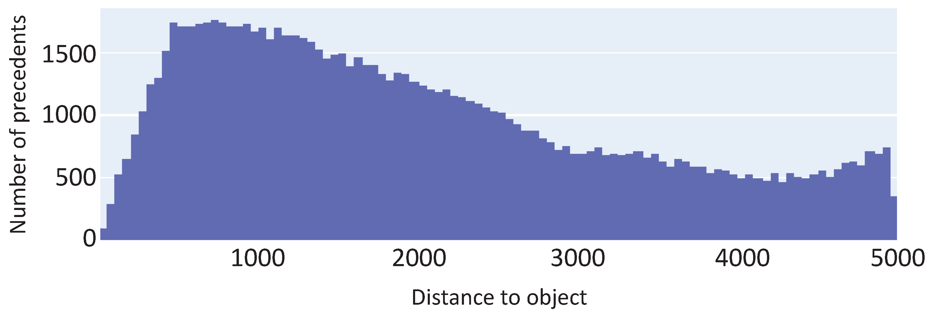
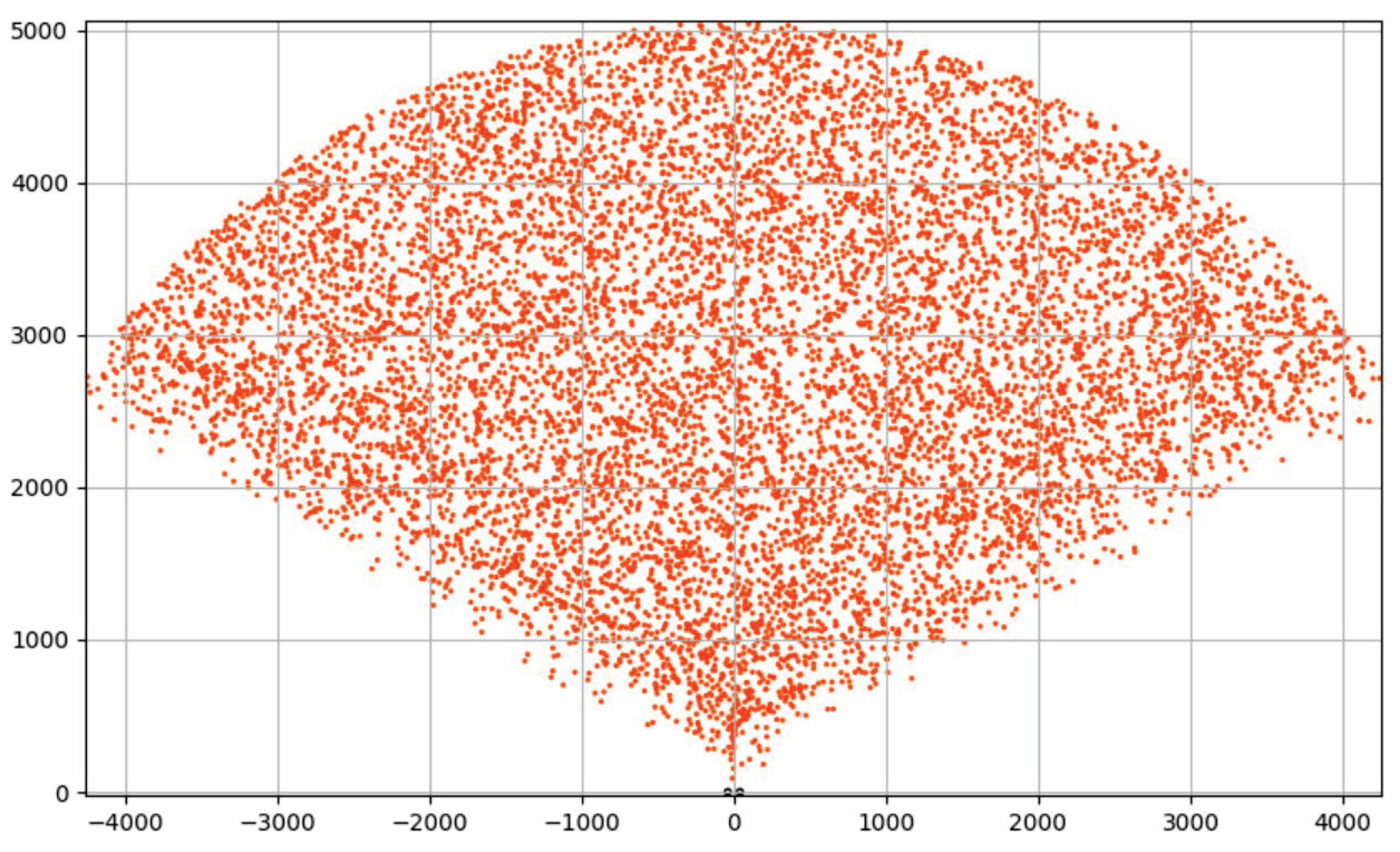
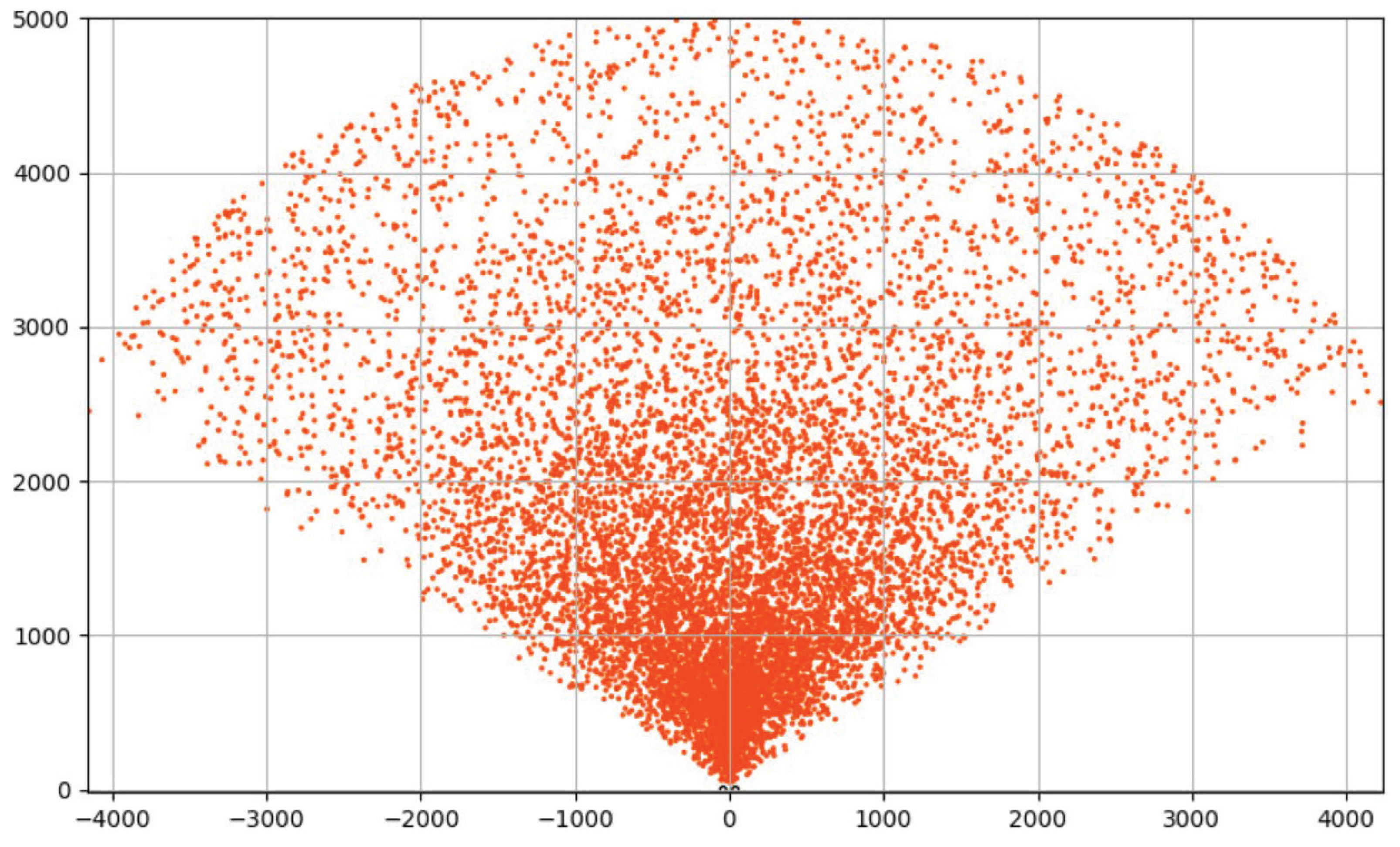
The histogram in Figure 8 shows that, after data set generation in one pass, most of objects accumulate in the interval $[500,3000]$ of distances to the observer. Such a skew can severely affect the quality of neural network training. The explanation of this anomaly is presented in Figure 10, which shows a diagram of the spatial distribution of object centers in the BFV zone after generation in one pass. For each orbit with radius r, Algorithm 1 generates approximately the same number of objects. However, the length of the orbit increases linearly with the growth of its radius. 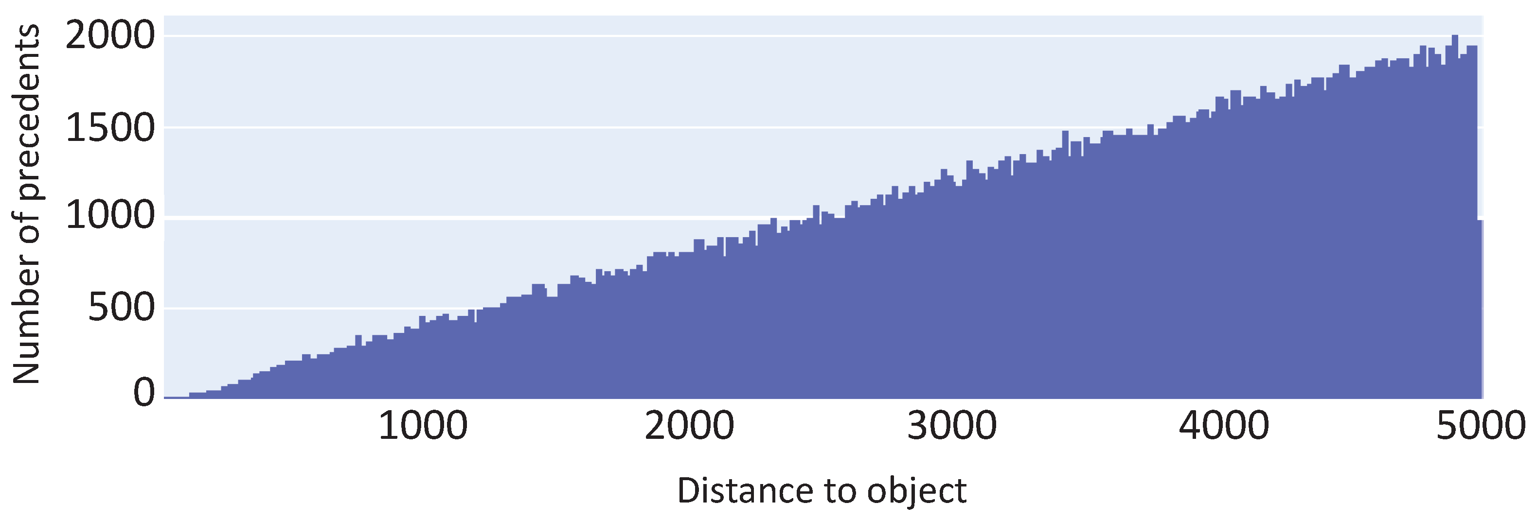Therefore, the density of objects decreases with increasing distance r from the observer. To overcome this issue, we used the method of multi-pass generation of the training data set. To do this, we divided the interval of values [0, 5000], specifying the distance to object, into 1000 segments of length 5. In each ith segment ($i=1,\dots ,1000$), using Algorithm 1, we generated $1000+200(i-1)$ precedents. In total, we received 100,900 precedents. The resulting distribution relative to the distance r to the object is shown in Figure 9; the spatial distribution of the observed object centers is shown in Figure 11. The data set generated in this way is freely available at https://github.com/artem-starkov/covidsgen/tree/main/dataset (accessed on 6 November 2021).

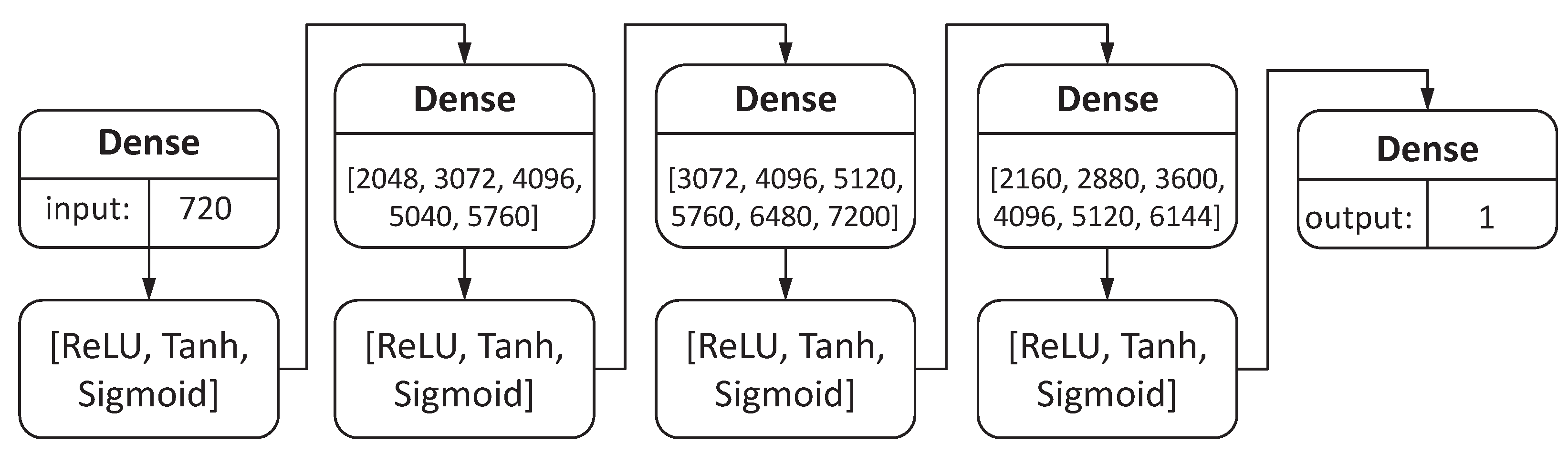
For the sake of simplicity, we decided to design two separate feedforward DNNs: the first to determine the distance and the second to determine the azimuth to a circular feature. To search for an optimal set of neural network hyperparameters, we constructed a common hypermodel for both networks. A diagram of the hypermodel is shown in Figure 12.

The hypermodel includes the input layer, three hidden layers, and the output layer. All of these layers are fully connected (have dense connections). For the input layer and all hidden layers, the activation functions to choose from are [ReLU, Tanh, Sigmoid]. The input layer has 720 neurons receiving external data: 360-bitmap from the left compound eye and 360-bitmap from the right compound eye. The output layer has a single neuron producing the ultimate result: the distance for the first DNN and the azimuth for the second DNN. For the first hidden layer, the numbers of neurons to choose from is [2048, 3072, 4096, 5040, 5760]. For the second and the third hidden layers, the numbers of neurons to choose from is [3072, 4096, 5120, 5760, 6480, 7200] and [2160, 2880, 3600, 4096, 5120, 6144], respectively.

Based on this hypermodel, we performed a limited random search for optimal sets of neural network hyperparameters using W&B [50]. As an optimization algorithm, we tested SGD (stochastic gradient descent) and RMSProp [51]. The batch size ranged from 4 to 64. As a loss function, we used MAE (mean absolute error) [52] calculated by the following equation:

$$MAE=\frac{1}{n}\sum _{i=1}^n\left|y_i-x_i\right|,$$

(33)

where n is the number of elements of the training data set, $y_i$ is the DNN output, and $x_i$ is the true value. The generated data set of 100,000 items was divided as follows:

• training sample: 68,000 items;
• validation sample: 12,000 items;
• test sample: 20,000 items.

The preliminary computational experiments with the hypermodel showed that a training sample with fewer than 60,000 items degrades the quality of training. For instance, a 50% reduction in the training sample results in a 20% decrease in detection accuracy. At the same time, an increase in the training sample of over 68,000 items does not improve accuracy.

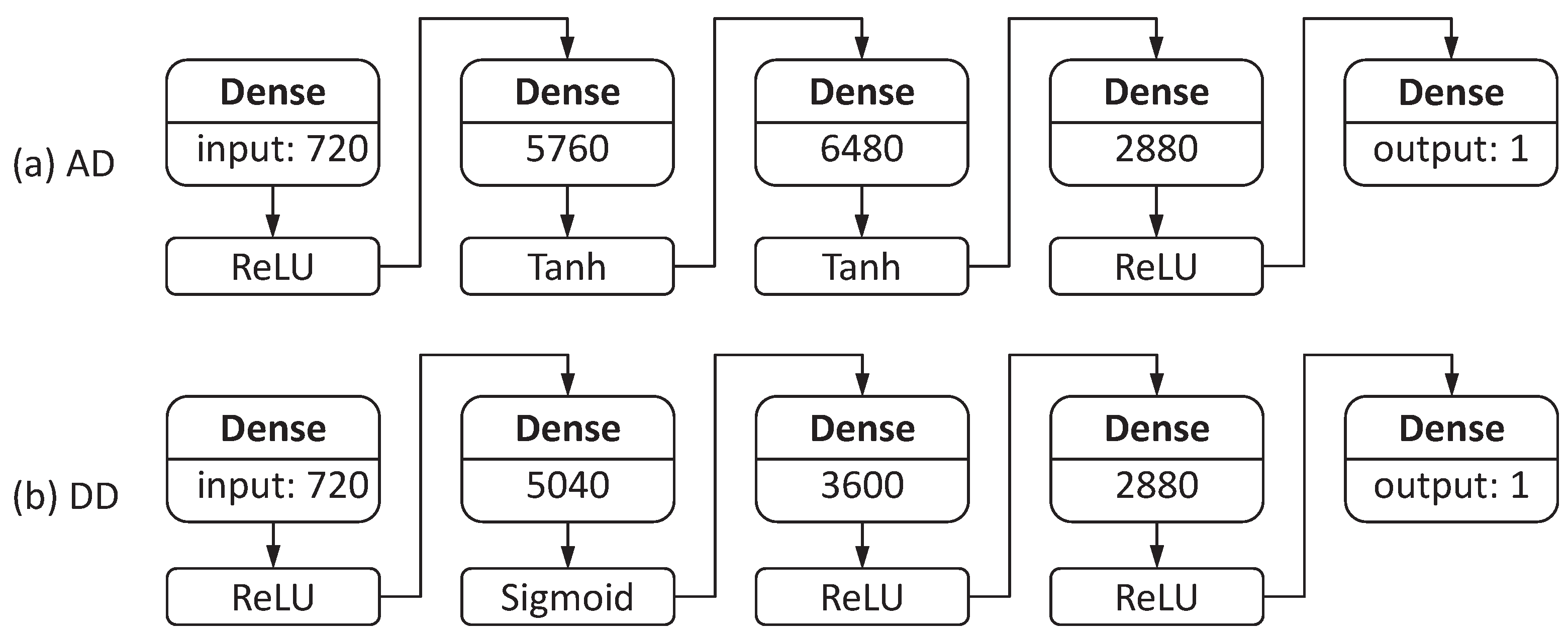
We used Keras and TensorFlow in Python to implement the hypermodel that was trained and tested on the Google Colab cloud platform [53] equipped with nVidia Tesla P4 graphics card. As a result, we obtained two DNNs shown in Figure 13.

The AD network includes the input layer, three hidden layers, and the output layer. The number of neurons in these layers is 720, 5760, 6480, 2880, and 1, respectively. All these layers are fully connected. For the input layer and the third hidden layer, the activation function is ReLU. For the thirst and second hidden layers, the activation function is Tanh. The input layer receives external data: 360-bitmap from the left compound eye and 360-bitmap from the right compound eye. The output layer produces the ultimate result: the azimuth to the object. The implementation of the AD network is presented in Appendix A.

Figure 13b illustrates the structure of the DD neural network that detects the distance to the object. The DD network includes the input layer, three hidden layers, and the output layer. The number of neurons in these layers is 720, 5040, 3600, 2880, and 1, respectively. All of these layers are fully connected. For the input layer, the second and third hidden layers, the activation function is ReLU. For the first hidden layer, the activation function is Sigmoid. The input layer receives the same external data: 360-bitmap from the left compound eye and 360-bitmap from the right compound eye. The output layer produces the ultimate result: the distance to the object. The implementation of the DD network is presented in Appendix B.

To assess the quality of the neural network models obtained, we used the following two metrics: MAPE (mean absolute percentage error) [54] defined by the equation

$$MAPE=\frac{100}{n}\sum _{i=1}^n\left|\frac{y_i-x_i}{x_i}\right|,$$

(34)

and the coefficient of determination $R^2$ [55] defined by the equation

$$R^2=1-\sum _{i=1}^n{\left(y_i-x_i\right)}^2/\sum _{i=1}^n{\left(y_i-y_{mean}\right)}^2,$$

(35)

where

$$y_{mean}=\frac{1}{n}\sum _{i=1}^n{y}_i.$$

(36)

The MAPE is often used in practice because of its very intuitive interpretation in terms of relative error. The coefficient of determination $R^2$ gives some information about the goodness of fit of a neural network model to the training data set. The models with $R^2>0.8$ can be considered quite good. The final training parameters and values of these metrics are presented in

Table 5. Final parameters of neural networks.

Parameter	Azimuth Detection	Distance Detection
Optimizer	RMSProp	SGD
Batch size	64	32
Learning rate	0.004	0.001
Training time	2 h 3 m 49 s	48 m 53 s
MAPE	0.832	7.713
$R^2$	0.998	0.899

.

6. Computational Experiments

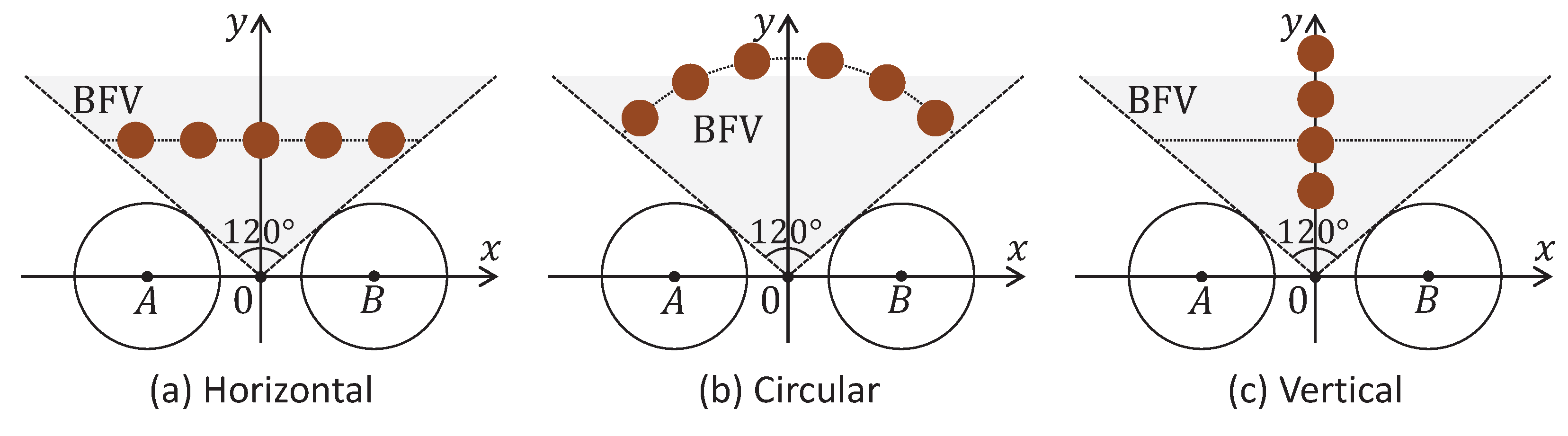
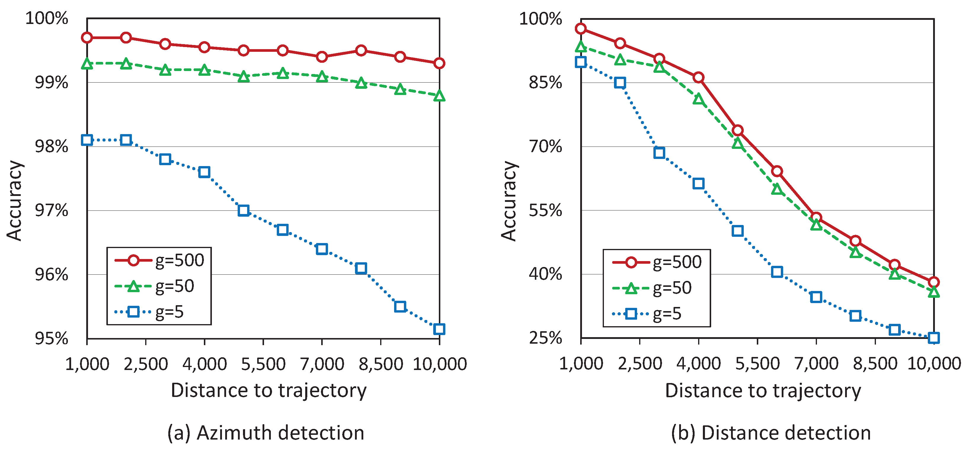
To test the accuracy of both designed neural network models, we performed a series of computational experiments. When developing the experiments, we took into account the following important point. It is well known that insects clearly see only moving objects [56]. The image motion can be a result of the movement of the object or the insect itself. The insect vision senses static images as a set of very blurred spots. Therefore, in our experiments, we simulated the movement of circular features of different radii along the three different trajectories shown in Figure 14.

The first type of trajectory is horizontal (see Figure 14a). Such trajectory is defined by a straight line parallel to the x-axis and located at a distance of r from the origin. The segment that is the intersection of this line with the BFV area has a length of $2tan\left({60}^{\circ }\right)r\approx 3.5r$. For this type of trajectory, we generated a set of circular features with a radius of g in the amount of $1.5r/g$, uniformly distributed along the trajectory. We fed the set of precedents constructed in this way to neural networks presented in Figure 13. The results for $g=5$, $g=50$, and $g=500$ are presented in Figure 15. Here and after $Accuracy=100\%-MAPE$. Diagram (a) in Figure 15 shows that the AD neural network (see Figure 13a) demonstrates great accuracy in determining an object’s azimuth. For all investigated trajectories, the accuracy of detecting the azimuth of large $(g=500)$ and medium $(g=50)$ objects is about 99%; for small objects $(g=5)$, the accuracy is more than 95%. Diagram (b) in Figure 15 shows the results obtained by the DD neural network (see Figure 13b) when detecting the distance to the object.

We can see that, in this case, the accuracy of determining the distance to large objects decreases from 98% to 74% with increasing distance to the trajectory from 1000 to 5000. In this interval, the accuracy decreases from 94% to 71% for medium objects and from 90% to 50% for small objects. Increasing the trajectory distance to 10,000, the accuracy of determining the distance to the object decreases to 38% for large objects, 36% for medium, and 25% for small. We should note that both neural networks learned at distances in the segment $[1000,5000]$. The experiments show that the AD neural network can work adequately at longer distances. This is explained by the fact that the object images shrink with increasing distance; small objects disappear, and large ones seem small. Therefore, the neural network can use the experience gained from training at shorter distances to detect azimuth at longer distances.

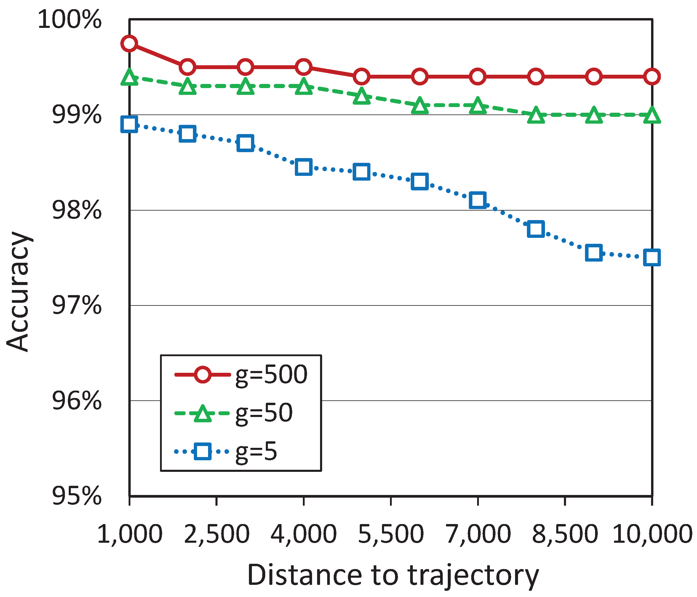
The second type of trajectory is circular (see Figure 14b). Such a trajectory is defined by a circle with radius r and the center at the origin. The arc that is the intersection of this circle with the BFV area has a length of $2\pi r120/360\approx 2.1r$. For this type of trajectory, we generated a set of circular features with a radius of g in the amount of $r/g$, uniformly distributed along the trajectory. We fed the set of precedents constructed in this way to the AD neural network (see Figure 13a). The results are presented in Figure 16.

We can see that the AD neural network demonstrates great accuracy in determining an object’s azimuth. For all investigated trajectories, the accuracy of detecting the azimuth of large $(g=500)$ and medium $(g=50)$ objects is more then 99%; for small objects $(g=5)$, the accuracy is more than 97%. The results obtained in this experiment look a little better than ones obtained when the object moves along a horizontal trajectory (see Figure 15a). This is because the ends of the horizontal segment of the trajectory are farther from the observer than its middle. In contrast, in the case of circular trajectory, the distance to the observer is always constant.

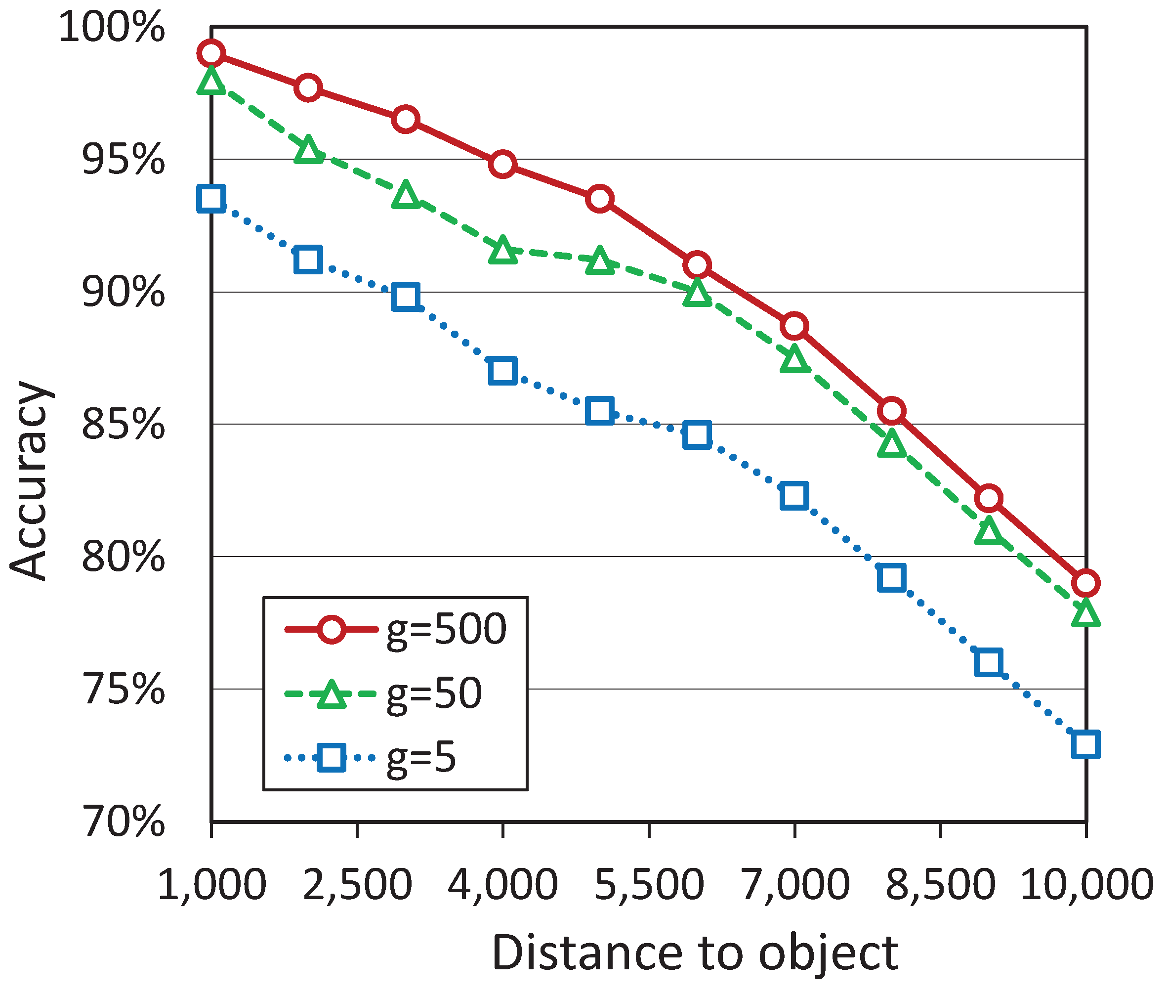
The third type of trajectory is vertical (see Figure 14c). Vertical trajectory coincides with the central axis of the BFV area. In our experiment, this trajectory has a length of 9000. For this type of trajectory, we generated a set of circular features with a radius of g in the amount of $4500/g$, uniformly distributed along the trajectory. We fed the set of precedents constructed in this way to the DD neural network (see Figure 13b). The results are presented in Figure 17.

The diagram shows that the accuracy of distance detection for all objects does not decrease below 70% in segment (1000, 10,000). Thus, the results obtained in this experiment look much better than ones obtained when the object moves along a horizontal trajectory (see Figure 15b). This is because the objects, in the case of vertical trajectory, are located on the central axis of the BFV area. We can conclude that to detect the distance to the object more accurately, the binocular compound eye vision system must turn frontally to the observed object.

Experiments showed that increasing the radius g of a circular feature improves the accuracy of determining the distance and azimuth. However, a tradeoff between size and accuracy is achieved when the dimensions of the object reach the boundaries of the BFV region (see Figure 5). Further expansion of the object size beyond the BFV region leads to a decrease in the accuracy of azimuth and distance measurements. In the extreme case, when the object completely overlaps the visible horizon, our neural networks can say nothing about the distance and azimuth to the object.

7. Discussion

In this section, we will discuss the following issues.

• What is the main contribution of this article?
• What are the advantages and disadvantages of the proposed approach compared to other known methods?
• Is the 2D model of compound eye vision applicable in practice?
• What are the future applications of the proposed model?
• What confirms the adequacy of the model?

Let us start answering the indicated questions. The main contribution of the article is a mathematical model of planar compound eye vision and a method for detecting the azimuth and distance to the observed object, which does not require the use of active sensors. Another important result is that DNNs based on the proposed model are able to detect azimuth and distance with high accuracy.

The advantage of the proposed method is a potentially more accurate measurement of azimuth and distance to the object compared to other known methods using passive sensors. The disadvantage of the described method is its inapplicability for the case when the observer and the object are static, relative to each other. Below, we explain why.

The 2D model of compound eye vision can be used to develop ground-based autonomous mobile robots. To operate on a surface, it is enough for the robot to have two planar compound eyes, each of which has one row of optical sensors (artificial ommatidia) installed in a circle. Similar implementations are known in the literature (see, for example, [13]). The optical sensor of the artificial compound eye transmits a signal to the neural network only when it detects an increase in light intensity. The signal will be especially strong if the adjacent optical sensor simultaneously detects a decrease in light intensity. In such a way, the neural network can sharply see the bounds of a moving object. That is why the object must move relative to the compound eye vision system in order to be detected.

The future applications of the proposed model are the following. First, the 2D model of compound eye vision can serve as a basis for designing physical optical systems for ground-based mobile robots. Such robots can participate in the mitigation of the consequences of accidents at nuclear power plants and extinguish fires at industrial facilities. Second, the proposed model makes it possible to construct an synthetic data set for prior supervised learning a neural network to detect the azimuth and distance to the observed object. After that, the pre-trained neural network is embedded in the physical prototype, and the final reinforcement learning is performed.

To confirm the adequacy of the developed model, we must implement it in the form of a physical prototype and check its operability. This is the subject of our future research. Nevertheless, when developing this model, we used the bionic principles inspired by the compound eyes of insects. To simulate a binocular compound eye system, we used the parameters comparable to the proportions of the robber fly vision system. This allows us to hope that the adequacy of the model will be confirmed in practice.

8. Conclusions

In this paper, we proposed a 2D model of the binocular compound eye vision inspired by insect eyes. The model includes two circular compound eyes located on a plane. The compound eye includes one row of ommatidia (optical sensors), arranged in a circle. The ommatidia are represented by equal-sized isosceles triangles. In the model, the ommatidium field of view is defined as a solid angle bounded by its legs. A ray tracing model was built on this basis. Using this model, an algorithm was developed for generating labeled data sets for training artificial neural networks capable of determining the distance and azimuth to the observed objects. Using the data sets generated by this algorithm, we designed and trained two feedforward deep neural networks: one to determine the distance and the other to determine the azimuth to circular features. To test the accuracy of both designed neural network models, we simulated the movement of circular features along different trajectories. Computational experiments have shown that the designed networks can detect azimuth with an accuracy of about 99% and the distance with an accuracy of about 80% for medium and large circular features.

Our future research directions on this subject are the following. We plan to investigate the dependence of the accuracy of azimuth and distance detection on the following parameters of the binocular compound eye vision system: the diameter of compound eyes, the distance between the eyes, and the number of ommatidia in the eye. We also plan to create a prototype of a planar binocular compound eye vision system to validate the described mathematical model. The same prototype will be used for reinforcement learning of the neural networks trained on synthetic data in the present study. Our next goal is to create and investigate a three-dimensional model of a binocular compound eye vision system focused on azimuth and distance detection.