Steady-State Solutions for Two Mixed Initial-Boundary Value Problems Which Describe Isothermal Motions of Burgers’ Fluids: Application

Abstract

Steady-state solutions of two mixed initial-boundary value problems are presented in equivalent forms. They describe isothermal permanent motions of incompressible Burgers’ fluids over an infinite flat plate that applies time-dependent shear stresses to the fluid. More exactly, they are the first exact solutions for motions of Burgers’ fluids with differential expressions of the shear stress or velocity on the boundary. The obtained results are designed to make equivalent solutions for motions caused by an infinite plate moving in its plane at velocities that seem to be similar to previous shear stresses. It is simple to limit all results for the purpose of providing efficient results for incompressible Oldroyd-B, Maxwell, second grade and Newtonian fluids undergoing comparable motions. They may also be used to estimate how long it will take to get to a steady or permanent state.

1. Introduction

The one-dimensional rate type fluid model proposed by Burgers [1] has often been used to describe the behavior of different viscoelastic materials such as polymeric liquids, cheese, soil and asphalt [2,3]. For instance, Lee and Markwick [4] reported that the behavior of asphalt and sand-asphalt and the predictions of their model agreed well. Additionally, this model was designed to describe the earth’s mantle’s ephemeral creep tendencies [5,6] and the fine-grained polycrystalline olivine’s high-temperature viscoelasticity [7,8]. Krishnan and Rajagopal have given a detailed analysis of the modeling, use and applications of asphalt concrete from antiquity to the present [9]. The same authors explored the expansion of Burgers’ model to a frame-indifferent three-dimensional form [10].

First exact steady solutions for isothermal motions of incompressible Burgers’ fluids are those obtained by Ravindran et al. [11] in an orthogonal rheometer. Hayat et al. [12] have derived steady-state solutions for periodic motions of the same fluid over an infinite plate or between parallel plates. Starting solutions for oscillatory motions (the second problem of Stokes) of incompressible Burgers’ fluids over an infinite moving plate, for instance, can be found in the references [13,14,15]. However, none of these solutions correspond to a motion in which a differential expression of the shear stress is given on the boundary.

The main purpose of this note is to present the first closed-form formulations for the dimensionless steady-state solutions corresponding to some motions of the incompressible Burgers’ fluids over an infinite flat plate. The novelty of this work consists in the consideration of the shear stress or velocity on the boundary of the flow domain as a time-dependent function defined as the sum between a decreasing exponential function and an oscillatory function with a given pulsation. The steady-state (permanent) solutions which are determined in this article are presented in elegant forms and are new in the literature. They correspond to isothermal motions of incompressible Burgers’ fluids for which differential expressions of shear stress or velocity are given on the boundary.

The solutions that have been obtained for motions with shear on the boundary are given in their most basic form and are easily particularized to provide the comparable responses for incompressible Oldroyd-B, Maxwell, second grade and Newtonian fluids flowing in a similar way. They may also be used to determine the time needed to attain the steady or permanent state, which is essential for experimentalists’ researchers in practice. Additionally, new precise solutions are developed for motions of the same fluids caused by the infinite plate that moves in its plane at velocities of the same form as the previous shear stresses. It is exploited by the fact that the governing equations of the fluid velocity and shear stress have identical forms.

2. Constitutive and Governing Equations

The constitutive equations of the incompressible Burgers’ fluids (IBF) are given by Equations.

$$\mathit{T}=-p\mathit{I}+{\widehat{\mathit{S}}}_1, {\widehat{\mathit{S}}}_1+\alpha \frac{D{\widehat{\mathit{S}}}_1}{D{\widehat{t}}_1}+\beta \frac{D^2{\widehat{\mathit{S}}}_1}{D{\widehat{t}}_1{}^2}=\mu \left({\widehat{\mathit{A}}}_1+\gamma \frac{D{\widehat{\mathit{A}}}_1}{D{\widehat{t}}_1}\right),$$

(1)

where $\mathit{T}$—Cauchy stress tensor, ${\widehat{\mathit{S}}}_1$—extra-stress tensor, I—unit tensor, ${\widehat{\mathit{A}}}_1={\widehat{\mathit{L}}}_1+{\widehat{\mathit{L}}}_1{}^T$ is the first Rivlin–Ericksen tensor (${\widehat{\mathit{L}}}_1$ being grad υ), $p$—hydrostatic pressure, $\mu$—fluid viscosity, $\alpha , \beta$ and $\gamma (\le \alpha )$ are material constants and $D/D{\widehat{t}}_1$—upper-convected derivative. The model defined by Equation (1) contains as particular cases the Oldroyd-B fluids if $\beta =0$, Maxwell fluids if $\beta =\gamma =0$ and Newtonian fluids if $\alpha =\beta =\gamma =0$. In some motions, the governing equations of second grade fluids can also be obtained as particular cases of the present equations. Since the incompressible fluids undergo isochoric motions only, it results in the following condition

$$\mathbf{tr} {\widehat{\mathit{A}}}_1=0 \mathrm{or} \mathrm{equivalently} \mathrm{div}\mathsf{\upsilon }=0,$$

(2)

having to be identically satisfied.

In the following, we shall consider isothermal unsteady motions of IBF over an infinite flat plate with velocity field:

$$\mathsf{\upsilon }=\mathsf{\upsilon }({\widehat{y}}_1,{\widehat{t}}_1)={\widehat{u}}_1({\widehat{y}}_1,{\widehat{t}}_1){\mathbf{e}}_{{\widehat{x}}_1},$$

(3)

where ${\mathbf{e}}_{{\widehat{x}}_1}$—unit vector along the ${\widehat{x}}_1$—direction of the Cartesian coordinate system (CCS) ${\widehat{x}}_1, {\widehat{y}}_1 \mathrm{and} {\widehat{z}}_1$ whose ${\widehat{y}}_1$—axis is perpendicular to the plate. At ${\widehat{t}}_1=0$, the fluid is at rest. We also assume that ${\widehat{\mathit{S}}}_1$, as well as υ, are functions of ${\widehat{y}}_1$ and ${\widehat{t}}_1$ only. Substituting the fluid velocity in Equation (1)₂ and bearing in mind that the fluid has been at rest at the initial moment ${\widehat{t}}_1=0$, it is easy to show that the components ${\widehat{S}}_{{\widehat{y}}_1{\widehat{y}}_1}, {\widehat{S}}_{{\widehat{y}}_1{\widehat{z}}_1}, {\widehat{S}}_{{\widehat{z}}_1{\widehat{z}}_1}$ and ${\widehat{S}}_{{\widehat{z}}_1{\widehat{x}}_1}$ of the ${\widehat{S}}_1$ are zero while the non-trivial shear stress ${\widehat{\tau }}_1({\widehat{y}}_1,{\widehat{t}}_1)={\widehat{S}}_{{\widehat{x}}_1{\widehat{y}}_1}({\widehat{y}}_1,{\widehat{t}}_1)$ has to satisfy the partial differential equation

$$\left(1+\alpha \frac{\partial }{\partial {\widehat{t}}_1}+\beta \frac{{\partial }^2}{\partial {\widehat{t}}_1{}^2}\right){\widehat{\tau }}_1({\widehat{y}}_1,{\widehat{t}}_1)=\mu \left(1+\gamma \frac{\partial }{\partial {\widehat{t}}_1}\right)\frac{\partial {\widehat{u}}_1({\widehat{y}}_1,{\widehat{t}}_1)}{\partial {\widehat{y}}_1}; {\widehat{y}}_1>0, {\widehat{t}}_1>0.$$

(4)

The incompressibility condition (2) is identically satisfied. When the body forces are conservative and there is no pressure gradient in the flow direction, the motion equations reduce to the following relevant partial differential equation

$$\frac{\partial {\widehat{\tau }}_1({\widehat{y}}_1,{\widehat{t}}_1)}{\partial {\widehat{y}}_1}=\rho \frac{\partial {\widehat{u}}_1({\widehat{y}}_1,{\widehat{t}}_1)}{\partial {\widehat{t}}_1}; {\widehat{y}}_1>0, {\widehat{t}}_1>0,$$

(5)

where $\rho$—constant density. The boundary conditions that will be used here are:

$$\left(1+\alpha \frac{\partial }{\partial {\widehat{t}}_1}+\beta \frac{{\partial }^2}{\partial {\widehat{t}}_1{}^2}\right){\widehat{\tau }}_1(0,{\widehat{t}}_1)=\mu \left(1+\gamma \frac{\partial }{\partial {\widehat{t}}_1}\right){\left.\frac{\partial {\widehat{u}}_1({\widehat{y}}_1,{\widehat{t}}_1)}{\partial {\widehat{y}}_1}\right|}_{{\widehat{y}}_1=0}={\widehat{S}}_1\cos (\omega {\widehat{t}}_1), \underset{{\widehat{y}}_1\to \infty }{\lim }{\widehat{u}}_1({\widehat{y}}_1,{\widehat{t}}_1)=0,$$

(6)

or

$$\left(1+\alpha \frac{\partial }{\partial {\widehat{t}}_1}+\beta \frac{{\partial }^2}{\partial {\widehat{t}}_1{}^2}\right){\widehat{\tau }}_1(0,{\widehat{t}}_1)=\mu \left(1+\gamma \frac{\partial }{\partial {\widehat{t}}_1}\right){\left.\frac{\partial {\widehat{u}}_1({\widehat{y}}_1,t_1)}{\partial {\widehat{y}}_1}\right|}_{{\widehat{y}}_1=0}={\widehat{S}}_1\sin (\omega {\widehat{t}}_1), \underset{{\widehat{y}}_1\to \infty }{\lim }{\widehat{u}}_1({\widehat{y}}_1,{\widehat{t}}_1)=0.$$

(7)

The second condition from the relations (6) and (7) tell us that the fluid is quiet far away from the plate. We also assume that there is no shear in the free stream, i.e.,

$$\underset{{\widehat{y}}_1\to \infty }{\lim }{\widehat{\tau }}_1({\widehat{y}}_1,{\widehat{t}}_1)=0.$$

(8)

The initial conditions ${\widehat{\tau }}_1(0,0)={\left.\frac{\partial {\widehat{\tau }}_1(0,{\widehat{t}}_1)}{\partial {\widehat{t}}_1}\right|}_{{\widehat{t}}_1=0}=0$ and the boundary conditions (6) and (7) imply for ${\widehat{\tau }}_1(0,{\widehat{t}}_1)$ the following expressions

$$\begin{array}{l}{\widehat{\tau }}_1(0,{\widehat{t}}_1)=\frac{(1-\beta {\omega }^2)\cos (\omega {\widehat{t}}_1)+\alpha \omega \sin (\omega {\widehat{t}}_1)}{{(\alpha \omega )}^2+{(1-\beta {\omega }^2)}^2}{\widehat{S}}_1\\ +\frac{{\widehat{S}}_1}{r_2-r_1}\left[\frac{\alpha {\omega }^2-r_2(1-\beta {\omega }^2)}{{(\alpha \omega )}^2+{(1-\beta {\omega }^2)}^2}{\mathrm{e}}^{r_1{\widehat{t}}_1}-\frac{\alpha {\omega }^2-r_1(1-\beta {\omega }^2)}{{(\alpha \omega )}^2+{(1-\beta {\omega }^2)}^2}{\mathrm{e}}^{r_2{\widehat{t}}_1}\right] ,\end{array}$$

(9)

respectively,

$$\begin{array}{l}{\widehat{\tau }}_1(0,{\widehat{t}}_1)=\frac{(1-\beta {\omega }^2)\sin (\omega {\widehat{t}}_1)-\alpha \omega \cos (\omega {\widehat{t}}_1)}{{(\alpha \omega )}^2+{(1-\beta {\omega }^2)}^2}{\widehat{S}}_1\\ +\frac{\omega {\widehat{S}}_1}{r_2-r_1}\left[\frac{\alpha r_2+1-\beta {\omega }^2}{{(\alpha \omega )}^2+{(1-\beta {\omega }^2)}^2}{\mathrm{e}}^{r_1{\widehat{t}}_1}-\frac{\alpha r_1+1-\beta {\omega }^2}{{(\alpha \omega )}^2+{(1-\beta {\omega }^2)}^2}{\mathrm{e}}^{r_2{\widehat{t}}_1}\right] ,\end{array}$$

(10)

where $r_{1,2}=(-\alpha \pm \sqrt{{\alpha }^2-4\beta })/(2\beta )$.

Consequently, the result is that the fluid motion is generated by the flat plate that applies a shear stress ${\widehat{\tau }}_1(0,{\widehat{t}}_1)$ of the form (9) or (10) to the fluid. If $\beta \to 0$, then $r_2\to -\infty , r_1\to -1/\alpha$ and the previous expressions take the simpler forms (see [16], Equations (5) and (6))

$${\widehat{\tau }}_1(0,{\widehat{t}}_1)=\left[\frac{\cos (\omega {\widehat{t}}_1)+\alpha \omega \sin (\omega {\widehat{t}}_1)}{{(\alpha \omega )}^2+1}-\frac{1}{{(\alpha \omega )}^2+1}\exp \left(-\frac{{\widehat{t}}_1}{\alpha }\right)\right]{\widehat{S}}_1,$$

(11)

$${\widehat{\tau }}_1(0,{\widehat{t}}_1)=\left[\frac{\sin (\omega {\widehat{t}}_1)-\alpha \omega \cos (\omega {\widehat{t}}_1)}{{(\alpha \omega )}^2+1}+\frac{\alpha \omega }{{(\alpha \omega )}^2+1}\exp \left(-\frac{{\widehat{t}}_1}{\alpha }\right)\right]{\widehat{S}}_1,$$

(12)

corresponding to similar motions of incompressible Maxwell and Oldroyd-B fluids. If both $\alpha$ and $\beta$ tend to zero, the plate applies an oscillatory shear stress

$${\widehat{\tau }}_1(0,t_1)={\widehat{S}}_1\cos (\omega {\widehat{t}}_1) \mathrm{or} {\widehat{\tau }}_1(0,{\widehat{t}}_1)={\widehat{S}}_1\sin (\omega {\widehat{t}}_1) ,$$

(13)

to the fluid. Such shear stresses are applied by the flat plate to incompressible second grade fluids if $\gamma$ is different to zero or to Newtonian fluids if $\gamma =0$.

3. Exact Steady-State Solutions

Let us introduce the following non-dimensional variables, functions and parameters in order to get exact results that are independent of the flow geometry.

$$\begin{array}{l}\mathsf{\Upsilon }={\widehat{y}}_1\sqrt{\frac{{\widehat{S}}_1}{\mu \nu }}, \mathfrak{J}=\frac{{\widehat{S}}_1}{\mu }{\widehat{t}}_1, \varpi ={\widehat{u}}_1\sqrt{\frac{\rho }{{\widehat{S}}_1}}, {\tau }^{\ast }=\frac{{\widehat{\tau }}_1}{{\widehat{S}}_1}, {\omega }^{\ast }=\frac{\mu }{{\widehat{S}}_1}\omega ,\\ {\alpha }^{\ast }=\frac{{\widehat{S}}_1}{\mu }\alpha , {\beta }^{\ast }=\frac{{\widehat{S}}_1{}^2}{{\mu }^2}\beta , {\gamma }^{\ast }=\frac{{\widehat{S}}_1}{\mu }\gamma .\end{array}$$

(14)

The dimensionless forms of the relations (4) and (5), namely

$$\left(1+\alpha \frac{\partial }{\partial \Im }+\beta \frac{{\partial }^2}{\partial {\Im }^2}\right)\tau (\mathsf{\Upsilon },\Im )=\left(1+\gamma \frac{\partial }{\partial \Im }\right)\frac{\partial \varpi (\mathsf{\Upsilon },\Im )}{\partial \mathsf{\Upsilon }}; \frac{\partial \tau (\mathsf{\Upsilon },\mathfrak{J})}{\partial \mathsf{\Upsilon }}=\frac{\partial \varpi (\mathsf{\Upsilon },\mathfrak{J})}{\partial \mathfrak{J}},$$

(15)

are immediately obtained using Equation (14) and dropping out the star notation. Eliminating $\tau (\mathsf{\Upsilon },\mathfrak{J})$ between the two relations (15), one obtains the next governing equation

$$\left(1+\alpha \frac{\partial }{\partial \mathfrak{J}}+\beta \frac{{\partial }^2}{\partial {\mathfrak{J}}^2}\right)\frac{\partial \varpi (\mathsf{\Upsilon },\mathfrak{J})}{\partial \mathfrak{J}}=\left(1+\gamma \frac{\partial }{\partial \mathfrak{J}}\right)\frac{{\partial }^2\varpi (\mathsf{\Upsilon },\mathfrak{J})}{\partial {\mathsf{\Upsilon }}^2}; \mathsf{\Upsilon }>0, \mathfrak{J}>0,$$

(16)

for the dimensionless velocity field $\varpi (\mathsf{\Upsilon },\mathfrak{J})$.

The corresponding dimensionless boundary conditions are

$$\left(1+\alpha \frac{\partial }{\partial \mathfrak{J}}+\beta \frac{{\partial }^2}{\partial {\mathfrak{J}}^2}\right)\tau (0,\mathfrak{J})=\left(1+\gamma \frac{\partial }{\partial \mathfrak{J}}\right){\left.\frac{\partial \varpi (\mathsf{\Upsilon },\mathfrak{J})}{\partial \mathsf{\Upsilon }}\right|}_{\mathsf{\Upsilon }=0}=\cos (\omega \mathfrak{J}), \underset{\mathsf{\Upsilon }\to \infty }{\lim }\varpi (\mathsf{\Upsilon },t)=0; \mathfrak{J}>0,$$

(17)

or

$$\left(1+\alpha \frac{\partial }{\partial \mathfrak{J}}+\beta \frac{{\partial }^2}{\partial {\mathfrak{J}}^2}\right)\tau (0,\mathfrak{J})=\left(1+\gamma \frac{\partial }{\partial \mathfrak{J}}\right){\left.\frac{\partial \varpi (\mathsf{\Upsilon },\mathfrak{J})}{\partial \mathsf{\Upsilon }}\right|}_{\mathsf{\Upsilon }=0}=\sin (\omega \mathfrak{J}), \underset{\mathsf{\Upsilon }\to \infty }{\lim }\varpi (\mathsf{\Upsilon },\mathfrak{J})=0; \mathfrak{J}>0.$$

(18)

The boundary conditions (17) and (18) and the fact that the fluid was at rest at the initial moment $\mathfrak{J}=0$, tell us that the two unsteady motions become permanent or steady in time. An important problem for such motions is to know the need time to reach the permanent or steady state. To determine this time, exact expressions have to be known for the transient or steady-state components of starting solutions. Unfortunately, there is no modality to verify the correctness of the transient solutions. This is the reason that we shall provide closed-form expressions for the steady-state solutions corresponding to the two motions in consideration. These solutions are independent of the initial conditions, but they satisfy the governing equations and boundary conditions. In order to avoid a possible confusion, we denote by ${\varpi }_{cp}(\mathsf{\Upsilon },\mathfrak{J})$, ${\tau }_{cp}(\mathsf{\Upsilon },\mathfrak{J})$ and ${\varpi }_{sp}(\mathsf{\Upsilon },\mathfrak{J})$, ${\tau }_{sp}(\mathsf{\Upsilon },\mathfrak{J})$ the permanent solutions corresponding to the partial differential Equation (16) with the boundary conditions (17), respectively (18).

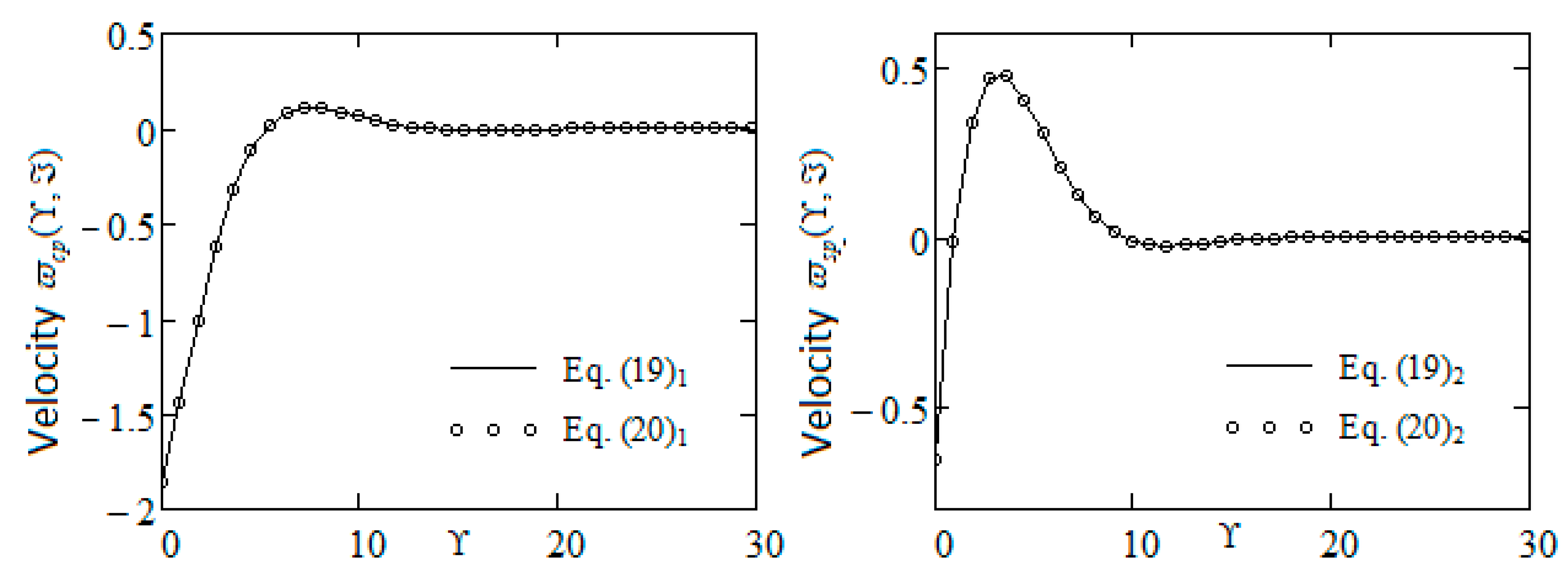
Direct computations show that the dimensionless velocity fields ${\varpi }_{cp}(\mathsf{\Upsilon },\mathfrak{J})$ and ${\varpi }_{sp}(\mathsf{\Upsilon },\mathfrak{J})$ corresponding to the two motions can be presented in the simple forms

$${\varpi }_{cp}(\mathsf{\Upsilon },\mathfrak{J})=-\Re e\left\{\frac{1}{(1+i\omega \gamma )\delta }{\mathrm{e}}^{-\delta \mathsf{\Upsilon }+i\omega \mathfrak{J}}\right\}, {\varpi }_{sp}(\mathsf{\Upsilon },\mathfrak{J})=-\mathrm{Im}\left\{\frac{1}{(1+i\omega \gamma )\delta }{\mathrm{e}}^{-\delta \mathsf{\Upsilon }+i\omega \mathfrak{J}}\right\},$$

(19)

or equivalently

$$\begin{array}{l}{\varpi }_{cp}(\mathsf{\Upsilon },\mathfrak{J})=-\sqrt{p^2+q^2} {\mathrm{e}}^{-\wp \mathsf{\Upsilon }}\cos (\omega \mathfrak{J}-\eta \mathsf{\Upsilon }+\varphi ),\\ {\varpi }_{sp}(\mathsf{\Upsilon },\mathfrak{J})=-\sqrt{p^2+q^2} {\mathrm{e}}^{-\wp \mathsf{\Upsilon }}\sin (\omega \mathfrak{J}-\eta \mathsf{\Upsilon }+\varphi ),\end{array}$$

(20)

where $\mathfrak{R}e$ and Im denote the real and the imaginary part, respectively, of that which follows.

$$\wp =\sqrt{\frac{\omega }{2}}\sqrt{\frac{a\omega +\sqrt{{\left(a\omega \right)}^2+b^2}}{1+{\left(\gamma \omega \right)}^2}}, \eta =\sqrt{\frac{\omega }{2}}\sqrt{\frac{-a\omega +\sqrt{{\left(a\omega \right)}^2+b^2}}{1+{\left(\gamma \omega \right)}^2}},$$

(21)

$$\begin{gathered} p=\frac{\omega \eta \gamma -\wp }{{(\omega \wp \gamma +\eta )}^2+{(\omega \eta \gamma -\wp )}^2}, q=\frac{\omega \wp \gamma +\eta }{{(\omega \wp \gamma +\eta )}^2+{(\omega \eta \gamma -\wp )}^2}, \\ \delta =\sqrt{i\omega (1-\beta {\omega }^2+i\omega \alpha )/(1+i\omega \gamma )}, a=\gamma (1-\beta {\omega }^2)-\alpha , b=1-\beta {\omega }^2+\alpha \gamma {\omega }^2, \varphi =\mathrm{arctg}(q/p) \end{gathered}$$

(22)

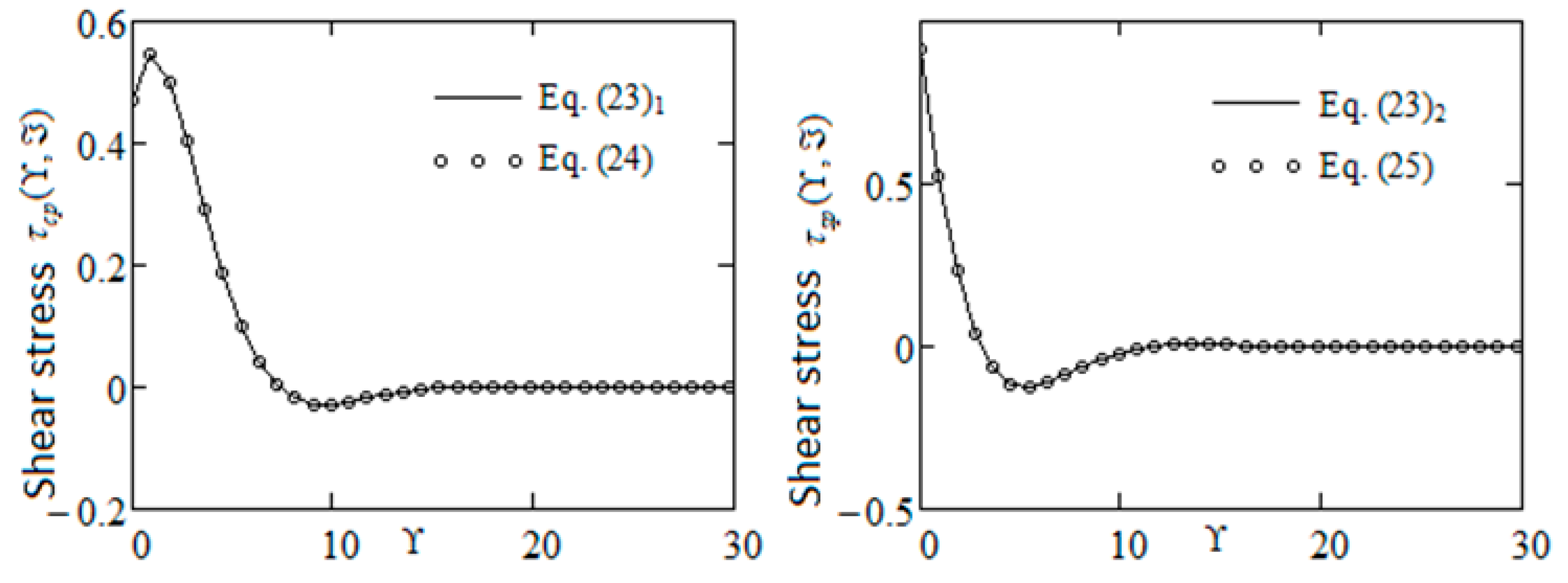
The corresponding shear stresses ${\tau }_{cp}(\mathsf{\Upsilon },\mathfrak{J})$ and ${\tau }_{sp}(\mathsf{\Upsilon },\mathfrak{J})$ are given by the relations

$${\tau }_{cp}(\mathsf{\Upsilon },\mathfrak{J})=\omega \mathfrak{R}e\left\{\frac{i}{(1+i\omega \gamma ){\delta }^2}{\mathrm{e}}^{-\delta \mathsf{\Upsilon }+i\omega \mathfrak{J}}\right\}, {\tau }_{sp}(\mathsf{\Upsilon },\mathfrak{J})=\omega \mathrm{Im}\left\{\frac{i}{(1+i\omega \gamma ){\delta }^2}{\mathrm{e}}^{-\delta \mathsf{\Upsilon }+i\omega \mathfrak{J}}\right\},$$

(23)

or equivalently

$${\tau }_{cp}(\mathsf{\Upsilon },\mathfrak{J})=\omega \sqrt{\frac{p^2+q^2}{{\wp }^2+{\eta }^2}} {\mathrm{e}}^{-\wp \mathsf{\Upsilon }}\cos (\omega \mathfrak{J}-\eta \mathsf{\Upsilon }+\varphi +\psi ),$$

(24)

$${\tau }_{sp}(\mathsf{\Upsilon },\mathfrak{J})=\omega \sqrt{\frac{p^2+q^2}{{\wp }^2+{\eta }^2}} {\mathrm{e}}^{-\wp \mathsf{\Upsilon }}\sin (\omega \mathfrak{J}-\eta \mathsf{\Upsilon }+\varphi +\psi ),$$

(25)

where $\psi =\mathrm{arctg}(\wp /\eta )$. Equivalence of the expressions of ${\varpi }_{cp}(\mathsf{\Upsilon },\mathfrak{J})$, ${\varpi }_{sp}(\mathsf{\Upsilon },\mathfrak{J})$ and ${\tau }_{cp}(\mathsf{\Upsilon },\mathfrak{J})$, ${\tau }_{sp}(\mathsf{\Upsilon },\mathfrak{J})$ given by Equation (19), respectively (23) to those from the equalities (20), (24) and (25), is graphically proved by Figure 1 and Figure 2.

Additionally, the exact solutions corresponding to incompressible Oldroyd-B, Maxwell, Newtonian or even second-grade fluids performing the same motions may be found straight immediately as limiting instances of the earlier discoveries. As an illustration, the dimensionless steady-state solutions for the isothermal motions of incompressible Newtonian fluids brought on by the flat plate that applies shear stresses to the fluid of type (13)

$$\begin{array}{l}{\varpi }_{Ncp}(\mathsf{\Upsilon },\mathfrak{J})=-\frac{1}{\sqrt{\omega }}\exp \left(-\mathsf{\Upsilon }\sqrt{\frac{\omega }{2}}\right)\cos \left(\omega \mathfrak{J}-\mathsf{\Upsilon }\sqrt{\frac{\omega }{2}}-\frac{\pi }{4}\right) ,\\ {\varpi }_{Nsp}(\mathsf{\Upsilon },\mathfrak{J})=-\frac{1}{\sqrt{\omega }}\exp \left(-\mathsf{\Upsilon }\sqrt{\frac{\omega }{2}}\right)\sin \left(\omega \mathfrak{J}-\mathsf{\Upsilon }\sqrt{\frac{\omega }{2}}-\frac{\pi }{4}\right),\end{array}$$

(26)

$$\begin{array}{l}{\tau }_{Ncp}(\mathsf{\Upsilon },\mathfrak{J})=\exp \left(-\mathsf{\Upsilon }\sqrt{\frac{\omega }{2}}\right)\cos \left(\omega \mathfrak{J}-\mathsf{\Upsilon }\sqrt{\frac{\omega }{2}}\right) ,\\ {\tau }_{Nsp}(\mathsf{\Upsilon },\mathfrak{J})=\exp \left(-\mathsf{\Upsilon }\sqrt{\frac{\omega }{2}}\right)\sin \left(\omega \mathfrak{J}-\mathsf{\Upsilon }\sqrt{\frac{\omega }{2}}\right) ,\end{array}$$

(27)

or equivalently

$${\varpi }_{Ncp}(\mathsf{\Upsilon },\mathfrak{J})=-\mathfrak{R}e\left\{\frac{1}{\sqrt{i\omega }}{\mathrm{e}}^{\sqrt{i\omega }(\mathfrak{J}\sqrt{i\omega }-\mathsf{\Upsilon })}\right\} , {\varpi }_{Nsp}(\mathsf{\Upsilon },\mathfrak{J})=-\mathrm{Im}\left\{\frac{1}{\sqrt{i\omega }}{\mathrm{e}}^{\sqrt{i\omega }(\mathfrak{J}\sqrt{i\omega }-\mathsf{\Upsilon })}\right\},$$

(28)

$${\tau }_{Ncp}(\mathsf{\Upsilon },\mathfrak{J})=\mathfrak{R}e\left\{{\mathrm{e}}^{\sqrt{i\omega }(\mathfrak{J}\sqrt{i\omega }-\mathsf{\Upsilon })}\right\} , {\tau }_{Nsp}(\mathsf{\Upsilon },\mathfrak{J})=\mathrm{Im}\left\{{\mathrm{e}}^{\sqrt{i\omega }(\mathfrak{J}\sqrt{i\omega }-\mathsf{\Upsilon })}\right\} ,$$

(29)

are immediately obtained taking $\alpha =\beta =\gamma =0$ in Equations (19), (20) and (23)–(25).

Finally, in order to use previous results to develop dimensionless steady-state solutions for other unsteady motions of the IBF, let us bring to light the fact that eliminating $\varpi (\mathsf{\Upsilon },\mathfrak{J})$ between Equation (15), one obtains for the corresponding shear stress $\tau (\mathsf{\Upsilon },\mathfrak{J})$, a partial differential equation identical in form with that of the fluid velocity, namely

$$\left(1+\alpha \frac{\partial }{\partial \mathfrak{J}}+\beta \frac{{\partial }^2}{\partial {\mathfrak{J}}^2}\right)\frac{\partial \tau (\mathsf{\Upsilon },\mathfrak{J})}{\partial \mathfrak{J}}=\left(1+\gamma \frac{\partial }{\partial \mathfrak{J}}\right)\frac{{\partial }^2\tau (\mathsf{\Upsilon },\mathfrak{J})}{\partial {\mathsf{\Upsilon }}^2}; \mathsf{\Upsilon }>0, \mathfrak{J}>0.$$

(30)

Consequently, the result is that the expressions of the dimensionless steady-state shear stresses ${\tau }_{cp}(\mathsf{\Upsilon },\mathfrak{J})$ and ${\tau }_{sp}(\mathsf{\Upsilon },\mathfrak{J})$ given by the relations (23)₁, (24), respectively (23)₂, (25) can be obtained solving the dimensionless differential Equation (30) with the boundary conditions

$$\left(1+\alpha \frac{\partial }{\partial \mathfrak{J}}+\beta \frac{{\partial }^2}{\partial {\mathfrak{J}}^2}\right)\tau (0,\mathfrak{J})=\cos (\omega \mathfrak{J}), \underset{\mathsf{\Upsilon }\to \infty }{\lim }\tau (\mathsf{\Upsilon },\mathfrak{J})=0; \mathfrak{J}>0,$$

(31)

respectively

$$\left(1+\alpha \frac{\partial }{\partial \mathfrak{J}}+\beta \frac{{\partial }^2}{\partial {\mathfrak{J}}^2}\right)\tau (0,\mathfrak{J})=\sin (\omega \mathfrak{J}), \underset{\mathsf{\Upsilon }\to \infty }{\lim }\tau (\mathsf{\Upsilon },\mathfrak{J})=0; \mathfrak{J}>0.$$

(32)

4. Application

Let us again consider an IBF at rest over an infinite flat plate which at the moment ${\widehat{t}}_1=0^{+}$ begins to move in its plane with a time-dependent velocity

$$\begin{array}{l}{\widehat{u}}_1(0,{\widehat{t}}_1)=\frac{(1-\beta {\omega }^2)\cos (\omega {\widehat{t}}_1)+\alpha \omega \sin (\omega {\widehat{t}}_1)}{{(\alpha \omega )}^2+{(1-\beta {\omega }^2)}^2}V\\ +\frac{V}{r_2-r_1}\left[\frac{\alpha {\omega }^2-r_2(1-\beta {\omega }^2)}{{(\alpha \omega )}^2+{(1-\beta {\omega }^2)}^2}{\mathrm{e}}^{r_1{\widehat{t}}_1}-\frac{\alpha {\omega }^2-r_1(1-\beta {\omega }^2)}{{(\alpha \omega )}^2+{(1-\beta {\omega }^2)}^2}{\mathrm{e}}^{r_2{\widehat{t}}_1}\right] ,\end{array}$$

(33)

or

$$\begin{array}{l}{\widehat{u}}_1(0,{\widehat{t}}_1)=\frac{(1-\beta {\omega }^2)\sin (\omega {\widehat{t}}_1)-\alpha \omega \cos (\omega {\widehat{t}}_1)}{{(\alpha \omega )}^2+{(1-\beta {\omega }^2)}^2}V\\ +\frac{\omega V}{r_2-r_1}\left[\frac{\alpha r_2+1-\beta {\omega }^2}{{(\alpha \omega )}^2+{(1-\beta {\omega }^2)}^2}{\mathrm{e}}^{r_1{\widehat{t}}_1}-\frac{\alpha r_1+1-\beta {\omega }^2}{{(\alpha \omega )}^2+{(1-\beta {\omega }^2)}^2}{\mathrm{e}}^{r_2{\widehat{t}}_1}\right] ,\end{array}$$

(34)

where V is a dimensional constant velocity.

Owing to the shear, the fluid is gradually moved and the corresponding velocity vector υ$({\widehat{y}}_1,{\widehat{t}}_1)$, reported to the same CCS as before, is again given by Equation (3). We also assume that the extra-stress tensor ${\widehat{\mathit{S}}}_1$ is a function of ${\widehat{y}}_1$ and ${\widehat{t}}_1$ only. Its components ${\widehat{S}}_{{\widehat{y}}_1{\widehat{y}}_1}, {\widehat{S}}_{{\widehat{y}}_1{\widehat{z}}_1}, {\widehat{S}}_{{\widehat{z}}_1{\widehat{z}}_1}$ and ${\widehat{S}}_{{\widehat{z}}_1{\widehat{x}}_1}$ are again zero and the dimensional fluid velocity ${\widehat{u}}_1({\widehat{y}}_1,{\widehat{t}}_1)$ together with the corresponding non-trivial shear stress ${\widehat{\tau }}_1({\widehat{y}}_1,{\widehat{t}}_1)$ satisfy the same partial differential Equations (4) and (5). The corresponding boundary conditions can be written in suitable forms

$$\left(1+\alpha \frac{\partial }{\partial {\widehat{t}}_1}+\beta \frac{{\partial }^2}{\partial {\widehat{t}}_1{}^2}\right){\widehat{u}}_1(0,{\widehat{t}}_1)={\widehat{V}}_1\cos (\omega {\widehat{t}}_1), \underset{{\widehat{y}}_1\to \infty }{\lim }{\widehat{u}}_1({\widehat{y}}_1,{\widehat{t}}_1)=0; {\widehat{t}}_1>0,$$

(35)

respectively

$$\left(1+\alpha \frac{\partial }{\partial {\widehat{t}}_1}+\beta \frac{{\partial }^2}{\partial {\widehat{t}}_1{}^2}\right){\widehat{u}}_1(0,{\widehat{t}}_1)={\widehat{V}}_1\sin (\omega {\widehat{t}}_1), \underset{{\widehat{y}}_1\to \infty }{\lim }{\widehat{u}}_1({\widehat{y}}_1,{\widehat{t}}_1)=0; {\widehat{t}}_1>0.$$

(36)

The following non-dimensional variables, functions and parameters are introduced

$$\begin{array}{l}\mathsf{\Upsilon }=\frac{{\widehat{V}}_1}{\nu }{\widehat{y}}_1, \mathfrak{J}=\frac{{\widehat{V}}_1{}^2}{\nu }{\widehat{t}}_1, \varpi =\frac{{\widehat{u}}_1}{{\widehat{V}}_1}, {\tau }^{\ast }=\frac{{\widehat{\tau }}_1}{\rho {\widehat{V}}_1{}^2}, {\omega }^{\ast }=\frac{\nu }{{\widehat{V}}_1{}^2}\omega ,\\ {\alpha }^{\ast }=\frac{{\widehat{V}}_1{}^2}{\nu }\alpha , {\beta }^{\ast }=\frac{{\widehat{V}}_1{}^4}{{\nu }^2}\beta , {\gamma }^{\ast }=\frac{{\widehat{V}}_1{}^2}{\nu }\gamma \end{array}$$

(37)

and again, abandoning star notation, one obtains for the two dimensionless entities $\varpi (\mathsf{\Upsilon },\mathfrak{J})$ and $\tau (\mathsf{\Upsilon },\mathfrak{J})$ partial differential equations of the forms (15). The velocity field $\varpi (\mathsf{\Upsilon },\mathfrak{J})$ also satisfies the partial differential Equation (16) which is identical in form with Equation (30).

The corresponding non-dimensional boundary conditions are

$$\left(1+\alpha \frac{\partial }{\partial \mathfrak{J}}+\beta \frac{{\partial }^2}{\partial {\mathfrak{J}}^2}\right)u(0,\mathfrak{J})=\cos (\omega \mathfrak{J}), \underset{\mathsf{\Upsilon }\to \infty }{\lim }\varpi (\mathsf{\Upsilon },\mathfrak{J})=0; \mathfrak{J}>0,$$

(38)

or

$$\left(1+\alpha \frac{\partial }{\partial \mathfrak{J}}+\beta \frac{{\partial }^2}{\partial {\mathfrak{J}}^2}\right)\varpi (0,\mathfrak{J})=\sin (\omega \mathfrak{J}), \underset{\mathsf{\Upsilon }\to \infty }{\lim }\varpi (\mathsf{\Upsilon },\mathfrak{J})=0; \mathfrak{J}>0.$$

(39)

Bearing in mind the results of the previous section, it is clear that the dimensionless velocity fields ${\varpi }_{cp}(\mathsf{\Upsilon },\mathfrak{J})$ and ${\varpi }_{sp}(\mathsf{\Upsilon },\mathfrak{J})$ corresponding to these motions are given by the following relations (see Equations (23)–(25))

$${\varpi }_{cp}(\mathsf{\Upsilon },\mathfrak{J})=\omega \mathfrak{R}e\left\{\frac{i}{(1+i\omega \gamma ){\delta }^2}{\mathrm{e}}^{-\delta \mathsf{\Upsilon }+i\omega \mathfrak{J}}\right\}, {\varpi }_{sp}(\mathsf{\Upsilon },\mathfrak{J})=\omega \mathrm{Im}\left\{\frac{i}{(1+i\omega \gamma ){\delta }^2}{\mathrm{e}}^{-\delta \mathsf{\Upsilon }+i\omega \mathfrak{J}}\right\},$$

(40)

or equivalently

$${\varpi }_{cp}(\mathsf{\Upsilon },\mathfrak{J})=\omega \sqrt{\frac{p^2+q^2}{{\wp }^2+{\eta }^2}} {\mathrm{e}}^{-\wp \mathsf{\Upsilon }}\cos (\omega \mathfrak{J}-\eta \mathsf{\Upsilon }+\varphi +\psi ),$$

(41)

$${\varpi }_{sp}(\mathsf{\Upsilon },\mathfrak{J})=\omega \sqrt{\frac{p^2+q^2}{{\wp }^2+{\eta }^2}} {\mathrm{e}}^{-\wp \mathsf{\Upsilon }}\sin (\omega \mathfrak{J}-\eta \mathsf{\Upsilon }+\varphi +\psi ),$$

(42)

where $\varphi$ and $\psi$ have already been defined.

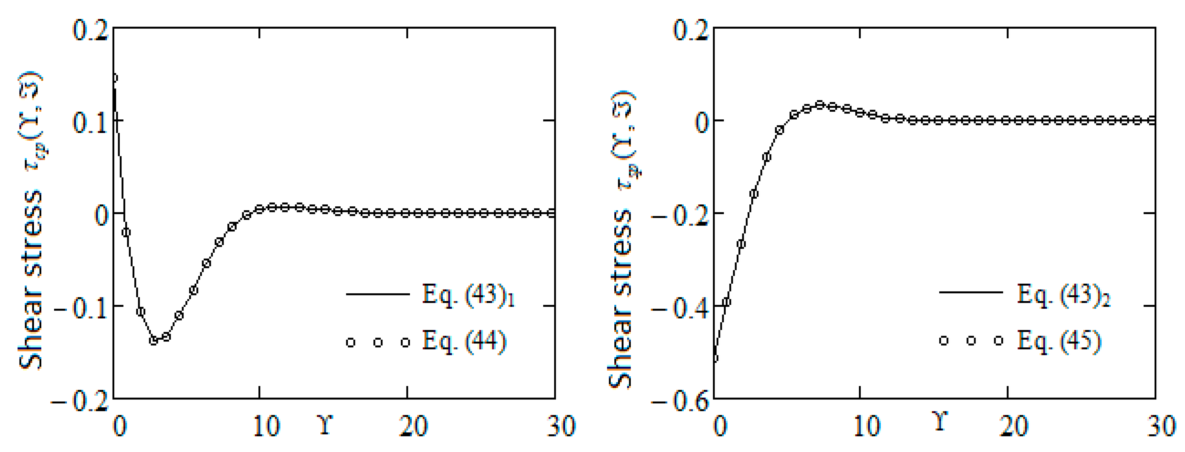
The corresponding shear stresses, namely

$${\tau }_{cp}(\mathsf{\Upsilon },\mathfrak{J})={\omega }^2\mathfrak{R}e\left\{\frac{1}{(1+i\omega \gamma ){\delta }^3}{\mathrm{e}}^{-\delta \mathsf{\Upsilon }+i\omega \mathfrak{J}}\right\}, {\tau }_{sp}(\mathsf{\Upsilon },\mathfrak{J})={\omega }^2\mathrm{Im}\left\{\frac{1}{(1+i\omega \gamma ){\delta }^3}{\mathrm{e}}^{-\delta \mathsf{\Upsilon }+i\omega \mathfrak{J}}\right\},$$

(43)

or equivalently

$${\tau }_{cp}(\mathsf{\Upsilon },\mathfrak{J})=-{\omega }^2\frac{\sqrt{p^2+q^2}}{{\wp }^2+{\eta }^2} {\mathrm{e}}^{-\wp \mathsf{\Upsilon }}\cos (\omega \mathfrak{J}-\eta \mathsf{\Upsilon }+\varphi +2\psi ),$$

(44)

$${\tau }_{sp}(\mathsf{\Upsilon },\mathfrak{J})=-{\omega }^2\frac{\sqrt{p^2+q^2}}{{\wp }^2+{\eta }^2} {\mathrm{e}}^{-\wp \mathsf{\Upsilon }}\sin (\omega \mathfrak{J}-\eta \mathsf{\Upsilon }+\varphi +2\psi ),$$

(45)

have been obtained using the relations (8) and (15)₂. The equivalence of the expressions of ${\tau }_{cp}(\mathsf{\Upsilon },\mathfrak{J})$ and ${\tau }_{sp}(\mathsf{\Upsilon },\mathfrak{J})$ given by Equation (43)₁, respectively (43)₂ to those from the equalities (44) and (45) is graphically proved by Figure 3.

Finally, taking $\alpha =\beta =\gamma =0$ in Equations (40)–(45), we recover the dimensionless steady-state solutions corresponding to isothermal motions of the incompressible Newtonian fluids generated by the flat plate that moves in its plane with the oscillatory velocities ${\widehat{V}}_1\cos (\omega {\widehat{t}}_1)$ or ${\widehat{V}}_1\sin (\omega {\widehat{t}}_1)$ (see [17], Equations (27)–(33)). The corresponding velocity fields, namely

$${\varpi }_{Ncp}(\mathsf{\Upsilon },\mathfrak{J})=\exp \left(-\mathsf{\Upsilon }\sqrt{\frac{\omega }{2}}\right)\cos \left(\omega \mathfrak{J}-\mathsf{\Upsilon }\sqrt{\frac{\omega }{2}}\right) ,{\varpi }_{Nsp}(\mathsf{\Upsilon },\mathfrak{J})=\exp \left(-\mathsf{\Upsilon }\sqrt{\frac{\omega }{2}}\right)\sin \left(\omega \mathfrak{J}-\mathsf{\Upsilon }\sqrt{\frac{\omega }{2}}\right) ,$$

(46)

are the dimensionless forms of the solutions (12) and (17) obtained by Erdogan [18].

5. Conclusions

The exact steady-state solutions to initial-boundary value problems often explain the motions or deformations of various fluids or solids. Additionally, they may be used as tests to validate numerical schemes created to research more difficult problems as well as to calculate the amount of time needed to reach the steady or permanent state. For two mixed initial-boundary value problems describing isothermal unsteady motions of IBF over an infinite flat plate when differential expressions of the shear stress are given on the boundary, we provided equivalent closed-form expressions for the dimensionless steady-state velocity and shear stress fields in this note.

The exact dimensionless steady-state solutions for unsteady motions of the same fluids over an infinite plate that move in its plane with time-dependent velocities of the same form as the previously applied shear stresses are developed using these solutions. They seem to be the first exact solutions of this type in the existing literature. All of the results found here may be easily customized to provide exact steady-state solutions for incompressible Oldroyd-B, Maxwell, second grade and Newtonian fluids acting in similar motions. For illustration, the corresponding solutions for isothermal unsteady motions of the incompressible Newtonian fluids due to the infinite plate that applies a shear stress ${\widehat{S}}_1\cos (\omega {\widehat{t}}_1)$ or ${\widehat{S}}_1\sin (\omega {\widehat{t}}_1)$ to the fluid are brought to light. The results that have been obtained here, especially the method used to find them, will be useful for establishing similar solutions for MHD motions of incompressible Burgers’ fluids through a porous media. The authors also believe that present results can be used to investigate flows of stratified fluids or nanofluids with Burgers’ fluids as base.