Abstract
In order to solve the problem in which structurally incoherent low-rank non-negative matrix decomposition (SILR-NMF) algorithms only consider the non-negativity of the data and do not consider the manifold distribution of high-dimensional space data, a new structurally incoherent low rank two-dimensional local discriminant graph embedding (SILR-2DLDGE) is proposed in this paper. The algorithm consists of the following three parts. Firstly, it is vital to keep the intrinsic relationship between data points. By the token, we introduced the graph embedding (GE) framework to preserve locality information. Secondly, the algorithm alleviates the impact of noise and corruption uses the L1 norm as a constraint by low-rank learning. Finally, the algorithm improves the discriminant ability by encrypting the structurally incoherent parts of the data. In the meantime, we capture the theoretical basis of the algorithm and analyze the computational cost and convergence. The experimental results and discussions on several image databases show that the proposed algorithm is more effective than the SILR-NMF algorithm.
MSC:
68U10
1. Introduction
In the past few decades, “curse of dimensionality” [1] problems have been a hot topic for many researchers. A popular dimensionality reduction method, 2D Local Preserving Projections (2DLPP) [2,3,4], has been widely utilized in pattern recognition [5,6,7] and computer vision [8,9,10]. However, on the basis of the 2DLPP unsupervised algorithm, some improved 2DLPP supervised algorithms have also been proposed [11,12,13].
Unfortunately, these above algorithms are similar in that they all use the L2 norm, which will hinder the algorithms’ performance when dealing with noise or abnormal data. Therefore, in order to solve the problem in which the L2 norm is affected by outliers, many researchers use L1-norm-based algorithms as dimension reduction algorithms of distance criteria, which are widely considered to be effective methods [14,15,16,17,18]. For example, L1-PCA [14] and PCA-L1 [15], based on the PCA algorithm, solve the noise and outlier sensitivity in the data through an optimization problem. Finally, the Rotation Invariant L1-norm PCA (R1-PCA) [16] algorithm proposed on the basis of L1-PCA has some PCA properties, which has some PCA properties. In order to solve the general L1 norm local preservation problem, Ref. [17] proposed the LPP algorithm (LPP-L1) based on the PCA-L1 algorithm to more effectively preserve the spatial topological structure. At the same time, in order to solve the outliers and corrosion problems in LPP-L1, a 2DLPP algorithm based on LPP-L1 algorithm (2DLPP-L1) was proposed [18].
In recent years, compared with algorithms based on L1 norm, many feature extraction algorithms using low rank representation (LRR) are conducive to extracting clean information, which has proved to be crucially important when there is noise in the data. The robustness of these algorithms has attracted considerable attention from researchers [19,20,21,22,23,24]. For example, in order to better maintain the lowest rank representation and global structure of data, the LRR in reference [19,20] introduced the single subspace clustering problem into multiple subspace clustering. The subspace structure was recovered from the data damaged by noise or occlusion. On the basis of LRR, a robust PCA (RPCA) was proposed by introducing kernel norm [21,22]. On the basis of LRR, the manifold structure was introduced as the regularization term, and Laplace regularization LRR [23] was proposed and applied to clustering data. Based on the combination of the NNLRS-graph and LRR, the non-negative concept was introduced to propose a non-negative low-rank sparse graph (NNLRS) [24] to maintain the global structure in the data.
A new matrix factorization method with structural incoherence (SILR-NMF) [25] has been introduced into face recognition to improve the recognition performance in the presence of corrupted data. In Ref. [26], a new structurally incoherent method was proposed to improve the additional discrimination ability in face recognition by introducing the structural incoherence. Motivated by [25] and [26], we propose a new algorithm dubbed structural incoherent low rank two-dimensional local discriminant mapping embedding (SILR-2DLDGE), which is superior to the SILR-NMF algorithm who has important limitations. Since the SILR-NMF algorithm can not make full use of the neighborhood relationship between data points. SILR-2DLDGE is implemented in three steps. Firstly, the intra-class weighted matrix graph and the inter-class weighted matrix graph are constructed to maintain the discriminant information of local neighborhood. Secondly, low-rank learning is used to eliminate noise and damage in the data. Finally, the structural incoherencies [25,26] are combined to optimize the discriminant information of different classes.
The four main contributions of this paper are as follows:
- We present a novel algorithm-based 2DLPP, which can simultaneously perform structurally incoherent, optimal graph Laplacian, and low-rank functions in a unified strategy. The algorithm has stronger discriminant ability than SILR-NMF, which fully reveals the structure information of the neighborhood to improve the discrimination ability.
- We propose to introduce intraclass and interclass graphs into the structurally incoherent model to make the data points in the same class more compact and different class data points as far away as possible.
- We used the low-rank feature to ensure that the given data are treated as two parts composed of the low-rank matrix and sparse matrix, representing useful features and nasty noise, respectively, so as to improve the performance of the algorithm using kernel norms as a measure of the regularization term.
- We designed a practical and simple algorithm to cater to the optimization process, and verified the algorithm on five datasets. Actually, our proposed method can achieve better performance.
The rest of study was planned as follows: Section 2 mainly introduces the early algorithms such as LRR, SILR-NMF, and LRMD-SI. Section 3 introduces the details of proposed algorithm, and analyzes the computational complexity and convergence of the SILR-2DLDGE algorithm. In Section 4, we compare the proposed algorithm with other state-of-the-art algorithms, and verify the promising performance of the SILR-2DLDGE algorithm on five databases. The summary and future work can be seen in the last section of the paper.
2. Related Works
2.1. Notation
To facilitate the understanding of this article, we will introduce the related work on some early algorithms, i.e., LRR, LRMD-SI, and SILR-NMF algorithms.
Firstly, we consider original space samples into feature space . Then, the linear transformation shown in Equation (1) can be obtained:
where is a transformation matrix, and .
Secondly, we define the matrix , and then or is used to represent the or row of , respectively.
Finally, we define the matrix , , and , respectively. Additionally, represents the kernel norm which is used to compute the sum of the singular matrix.
2.2. LRR
The LRR [19] algorithm is different from sparse representation [27]. LRR adopts a joint approach to transfer the recovery of damaged data to multiple subspaces, which is an effective subspace segmentation algorithm. At the same time, the global structure of data is obtained by searching the lowest rank representation of all data.
Each data vector in can be learned by the linear combination of the :
where is the coefficient matrix being, representation :
Here, denotes the nuclear norm.
The noise E can be separated from corrupted data as follows [19]:
where is a parameter.
2.3. SILR-NMF
In view of the fact that face is often affected by noise, SILR-NMF [25] is a better choice for feature representation and image classification. We can obtain Equation (5) as the final form of its objective function:
where , , and are positive parameters.
2.4. LRMD-SI
In view of the fact that face is often affected by noise, Wei et al. [26] introduced a structurally incoherent constraint based on low-rank matrix decomposition (LRMD-SI), which is considered to have good performance in image representation and classification. We can obtain Equation (6) as the final form of its objective function:
where matrix is the F-norm of the matrix, is the parameter, and .
3. Structurally Incoherent Low-Rank 2D Local Discriminant Graph Embedding
This section discusses the objective function of the SILR-2DLDGE algorithm, and describes its optimization process, computational complexity, and convergence.
3.1. The Objective Function of SILR-2DLDGE
In low-rank matrix recovery, the training dataset , which is divided into the low-rank matrix and the noise matrix , where , is the number of class of training sample , and N is the total number of data in the class of training sample . Then, we have the following:
where is a parameter.
The following equation can be obtained by encoding the 2DLDGE algorithm into Equation (10) and introducing an orthogonal constraint on :
where the balance parameters and .
We define the scatter matrix (intra-class) and the scatter matrix (inter-class) in Equation (8):
where or in the same class means the index set of the Kc nearest neighbors of the sample or , respectively. Additionally, or in the different class express the index set of the Kb nearest neighbors of the sample or , respectively.
We added structural incoherence to Equation (8), which is expressed as follows to improve the discrimination ability and further distinguish the different classes of the Equation (7) algorithm:
In Equation (11), the algorithm improves the incoherence of algorithm structure by adding the F-norm between different pairs of and . The first term is to maintain the neighborhood information in the low dimensional subspace consistent with the clean data structure. The second term is used to learn a low rank matrix to ensure that its noise interference is reduced as much as possible. The last term has the discrimination ability and further distinguishes the different classes in the data.
3.2. The Optimization of SILR-2DLDGE
Due to the product term , the minimization Equation (11) is non-convex. We iteratively replaced low-rank matrices to solve the following problems:
By introducing the auxiliary variable to solve Equation (12), the following equation can be obtained:
Augmented Lagrange multipliers or ADMM [28] and other techniques can be used to solve Equation (13). We solved Equation (13) by performing singular value decomposition (SVD) at each iteration step, but it may have high computational complexity. We used the nuclear norm property [29] to reduce the complexity of Equation (13) as follows [30]:
where is an arbitrary matrix. If of , the factorization is obtained by the minimum solution of the above equation.
We can write the equivalent of Equation (13) using the conclusion of Equation (14) as follows:
The augmented Lagrange function of Equation (15) is detailed as follows:
where the penalty parameter is , and the Lagrange multipliers are , , and .
Next, we separated the solutions for each variable.
- (1)
- Fix , , , , and , and update : since , , , , and are fixed, we can obtain the following equation from Equation (16):
Letting the partial derivative of variable B be zero in Equation (17):
Then, we have the following:
- (2)
- Fix , , , , and , and update : by fixing other variables, we can obtain the following equation from Equation (16):
In Equation (20), letting the partial derivative of be zero, we have:
where , and .
- (3)
- Fix , , , , and , and update : to fix other variables, the optimal can be obtained in Equation (16); thus, we have:
To simplify the solution of the above problem, we introduce a shrinkage operator according to reference [31]. In addition, represents the soft threshold to achieve the above purposes [32]. Finally, it is converted into Equation (23):
- (4)
- Fix , , , , and , and update : we obtain the following Equation (24) by fixing all variables except in Equation (16):
In Equation (24), letting the partial derivative of variable be zero, we obtain:
- (5)
- Fix , , , , and , and update : we fix all other variables in Equation (16) except ; thus, the following equation can be obtained:
The following equation is obtained to use the partial derivative of Equation (26):
- (6)
- Fix , , , , and , and update : we simplify Equation (16) and obtain the solution of variable :
In order to solve the equation better, we add a constraint adjustment; the equation is as follows:
Equations (29) and (30) can be transformed into the following formula:
The solution of Equation (31) is the same as solving the generalized eigenvalue equation as follows:
Algorithm 1 gives the concrete steps of SILR-2DLDGE.
| Algorithm 1 SILR-2DLDGE |
| Input: Parameters , , and ; and Training set X in Equation (14). Initialization: = 0, = 0, > 0, = 0, = 0, = 0. Repeat Step 1. Fixing , , , and , update with Equation (17); Step 2. Fixing , , , and , update with Equation (20); Step 3. Fixing , , , and , update with Equation (22); Step 4. Fixing , , , and , update with Equation (24); Step 5. Fixing , , , and , update with Equation (26); Step 6. Fixing , , , and , update with Equation (28); Step 7. Update parameter , , and as follows: Update through ; Update through ; Update through ; Step 8. Update through ; Step 9. Update through t = t + 1; Until Equation (11) is converged. Step 10. Obtain the (, , , , , ) optimal solution; Output: Obtain projection matrix |
The flow chart of the SILR-2DLDGE method is shown in Figure 1.
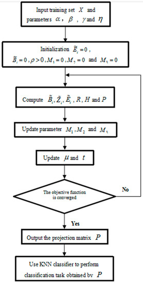
Figure 1.
The flow chart of the SILR-2DLDGE method.
3.3. The Convergence Analysis
Firstly, we analyzed and proved the weak convergence of the proposed SILR-2DLDGE algorithm. In some cases, any limit point of the iterative sequence generated by the SILR-2DLDGE algorithm is a stationary point satisfying the Karush–Kuhn–Tucker (KKT) condition [33].
Assuming that the SILR-2DLDGE algorithm reaches a stationary point, any convergence point must satisfy the KKT condition, which is a necessary condition for a local optimal solution. Therefore, we can derive the KKT condition of Equation (11) as follows (note that Lagrange multiplier is not involved in the process of solving ; thus, we do not prove its KKT condition):
It can be deduced from the last relationship in Equation (33) that:
where the application element to is the scalar function . From [34], the following relationships will be learned:
where . Thus, the following equation can be obtained with the KKT condition:
On the basis of the above conditions, the point convergence satisfying the KKT condition is proved.
Theorem 1 [25].
Suppose that is bounded to be generated by the SILR-2DLDGE algorithm and let. Ifsatisfies KKT conditions and converges, then it can be obtained that any point converges to the KKT point in.
Proof of Theorem 1.
is the next point of in the sequence . Firstly, , , and can be obtained, as shown in the following equation:
If , and , then we can obtain that , and . Thus, the sequence variables of , and converge to the stationary point, and we obtain the first three conditions in Equation (37).
Next, according to the SILR-2DLDGE algorithm and the fourth KKT condition, we obtain Equation (38):
When , we can derive from the second condition.
The following equation is obtained by the third KKT condition:
Thus, when .
Similarly, the following equation can be obtained:
When , can be obtained. Similarly:
When , we have .
From the last condition in Equation (35), the following equation is as follows:
We can obtain the last condition when .
Both sides of Equations (38)–(42) indicate tending to 0 when . Finally, the sequence variable of can be obtained asymptotically to satisfy the KKT condition in Equation (11).
QED □
3.4. Computational Complexity
The main computation steps of SILR-2DLDGE algorithm are shown in steps 2 and 6. In the SILR-2DLDGE algorithm, the complexity of step 2 is O(t(2a2l)) to solve the Sylvester equation problem, and the complexity of step 6 is O(t(2a3)). Therefore, we can obtain the total complexity of the SILR-2DLDGE algorithm, which is O(t(2(a3 + a2l))), where t is the number of iterations.
4. Experiment Results
In this section, we introduce several representative experiments to verify the robustness of the proposed SILR-2DLDGE algorithm. We compared the results of the proposed algorithm with 2DLPP [2,3,4], LPP-L1 [17], 2DLP-L1 [18], LRR [19,20], SILR-NMF [25], LRMD-SI [26], and LPP [35,36] algorithms on FERET [37], ORL [38], coil100 [39], Yale [40], AR [41], and PolyU [42] databases, respectively.
4.1. Selection of Samples and Parameters
In each subsequent experiment, we will randomly select T = 5, 6, 10, 5, 6, 3 samples from each class in FERET, ORL, COIL 100, Yale, AR, and PolyU databases for training. In each running experiment, NN classifier was used for classification, and the experiment was repeated 10 times.
In all the following experiments, we used an iterative algorithm to derive solutions of the L1-norm algorithms and set the maximum value of iterations of the relevant iterative algorithm to 500. The LPP, 2DLPP, LPP-L1, and 2DLPP-L1 algorithms based on local graph embedding are obtained using k-nearest neighbors, where k = T − 1 (T is the training sets of each databases) is well collected in the observation space [43]. We choose the parameters of LRR, LRMD-SI, and SILR-NMF models in the references. From the objective function of the SILR-2DLDGE algorithm in Equation (13), the parameter range of α, β, and η were selected from [0.001, 0.01, 0.1, 1, 10, 100, 1000], and the γ parameter was selected from [0.1, 0.2, ……, 0.9, 1] to evaluate the effect, the values of parameters in our algorithm are given in Table 1.

Table 1.
Parameter values of the SILR-2DLDGE algorithm on different datasets.
4.2. Experiments on Occlusion Databases
To verify the robustness of the algorithm, we will randomly add 10 × 10 blocks to different positions of images to carry out continuous occlusion experiments in FERET, ORL, and COIL100 databases.
- FERET database
The FERET database is mainly used to study changes in pose, illumination, and facial expression. There are 200 classes in the FERET database, and each class has seven images with a resolution of 40 × 40 pixels, resulting in a total of 1400 gray-scale images.
- ORL database
The ORL database is mainly used to study changes with different expressions, postures, and illuminations. There are 40 classes in the ORL database., and each class has 10 images with a resolution of 56 × 46 pixels, resulting in a total of 400 gray-scale images.
- COIL 100 database
The COIL 100 object database is mainly used to study changes with different illuminations. There are 100 subjects, and each subject has 72 images with a resolution of 32 × 32 pixels, resulting in a total of 7200 gray-scale images. Figure 2 shows some occlusion images on the three different databases.
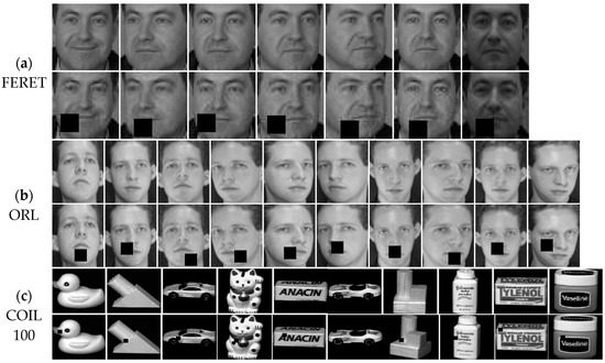
Figure 2.
Some occlusion images from the three different databases. (a) FERET, (b) ORL, and (c) COIL 100.
To verify the effectiveness of continuous occlusion in FERET, ORL, and COIL100 databases, respectively, we randomly added 10 × 10 blocks to different positions of images. Figure 3, Figure 4 and Figure 5 show the average recognition rates (%) of different dimension changes on the three different databases.
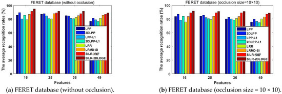
Figure 3.
The average recognition rates (%) of the eight algorithms in the FERET database vary with the dimension.
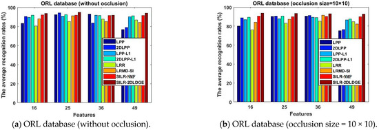
Figure 4.
The average recognition rates (%) of the eight algorithms in the ORL database varies with the dimension.
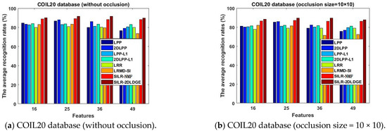
Figure 5.
The average recognition rates (%) of the eight algorithms in COIL20 database vary with the dimension.
We ran a set of experimental results and compared them with seven methods; the results are presented in this section. According to the settings in Section 4.1, when each class in FERET, ORL, and COIL100 databases randomly selects T sample points to form a training sample set, the optimal average recognition rate (%) of the seven algorithms is shown in Table 2.
Table 2.
The best average recognition rates (%) of the eight algorithms in FERET, ORL, and COIL100 databases and the corresponding dimensions (D).
4.3. Experiments on Noise Databases
Experiments were carried out on different levels of random pixel corruptions to verify the robustness of the algorithm. “Salt & pepper” noise with a density of 0.1 was added to the Yale, AR, and PolyU databases for corrosion experiments.
- Description of the Yale database
The Yale face database is mainly used to study changes in facial expressions and lighting conditions. There are 15 classes in the Yale database, and each class has 11 images with a resolution of 50 × 40 pixels, resulting in a total of 165 gray-scale images.
- Description of the AR database
The AR database is mainly used to study the changes in lighting conditions, facial expressions, and occlusion. There are 70 men and 56 women with a total of 126 people in the AR database, including 4000 color images with a resolution of 50 × 40 pixels.
- Description of the PolyU palmprint database
The PolyU database is mainly used to study image changes in two periods. There are 100 different palms in the PolyU database, and each palm has six samples, resulting in a total of 600 gray images with a resolution of 64 × 64 pixels. Figure 6 shows the original images and some corrosion images on the three different databases.
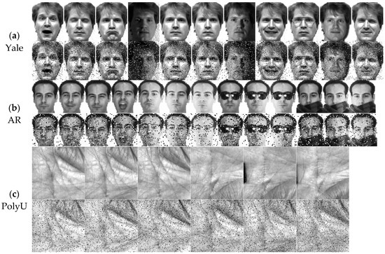
Figure 6.
Some the original images and corrosion images on the three different databases. (a) Yale, (b) AR, and (c) PolyU.
For continuous corrosion experiments, we randomly added a density of 0.1 of “salt & pepper” noise to the Yale, AR, and PolyU databases. Then, we ran a set of experiments and compared them with seven methods to evaluate the proposed SILR-2DLDGE algorithm. Figure 7, Figure 8 and Figure 9 show the average recognition rates (%) of different dimension changes on the three different databases.
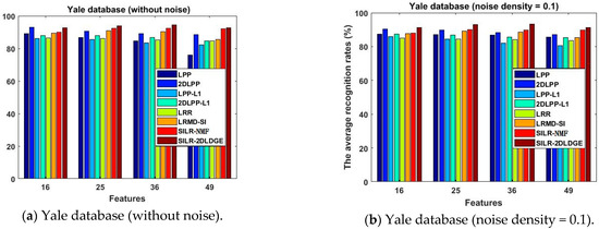
Figure 7.
The average recognition rates (%) of the eight algorithms in the Yale database vary with the dimension.
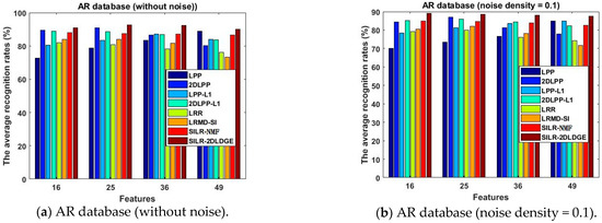
Figure 8.
The average recognition rates (%) of the eight algorithms in the AR database vary with the dimension.
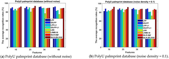
Figure 9.
The average recognition rates (%) of the eight algorithms in the PolyU palmprint database vary with the dimension.
As in the last experiment, we can obtain the best average recognition rates (%) of the eight algorithms according to the settings in Section 4.1, as shown in Table 3.
Table 3.
The best average recognition rates (%) of different algorithms and corresponding dimensions (D) on the Yale, AR, and PolyU databases and the corresponding dimensions.
4.4. Convergence Study
In the last experiment, we will further prove the convergence of the SILR-2DLDGE algorithm on the FERET and AR databases, respectively. The objective function values decreased monotonically; Figure 10 shows that the proposed algorithms are convergent due to the increase in the number of iterations.
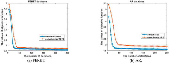
Figure 10.
Convergence of the proposed algorithm. (a) FERET databases; (b) AR databases.
In addition, to further verify the effectiveness of our proposed algorithm, we took the first three training samples from each class on the PolyU palmprint database; Table 4 shows the CPU time of each method.
Table 4.
The average CPU time consumed of the eight algorithms in the PolyU palmprint database.
4.5. Observations and Discussion
The four contributions of the SILR-2DLDGE algorithm are as follows:
- (1)
- In Table 2 and Table 3, the maximum average recognition rate of the SILR-2DLDGE algorithm on different databases is the highest, which fully shows that our algorithm is optimal and robust. The key reason is that SILR-2DLDGE not only learns a base matrix with low-rank property and local discriminant ability, but also has the advantages of SILR-NMF, which can weaken the disturbance of noise.
- (2)
- The SILR-2DLDGE algorithm has the advantages of low-rank learning, sparse learning, and incoherent structure learning, similarly to the SILR-NMF algorithm, as well as the advantages of graph embedding, which shows that more discrimination information can be obtained by sparse learning combined with the L1 norm and L * norm. We can see from the curve changes in Figure 3, Figure 4, Figure 5, Figure 7, Figure 8 and Figure 9 that the average recognition rates of this algorithm in three noisy databases and three occlusion databases are higher than that of other algorithms, which fully show that our algorithm has stronger robustness than other algorithms.
- (3)
- The SILR-2DLDGE algorithm takes less time than the others (Table 4) and learns the sparse transformation matrix to encode the geometric structure of the data and effectively improve the classification accuracy, which can obtain clean data in cases of noise disturbance. At the same time, structural incoherence can ensure that it is easier to separate data points of different classes.
- (4)
- The maximum average recognition rate of the SILR-2DLDGE algorithm varies among different databases. For example, the SILR-2DLDGE algorithm has the highest average maximum recognition rate without occlusion on the ORL database, whereas it has the lowest average maximum recognition rate with an occlusion of 10 × 10 on the COIL20 database. At the same time, the SILR-2DLDGE algorithm has the highest average maximum recognition rate without noise on the YALE database, whereas it has the lowest average maximum recognition rate with added “salt and pepper” noise with a density of 0.1 on the AR database. The above reasons are due to the small number of ORL and YALE samples, the large AR and PolyU palmprint databases, the presence of glasses and other occlusions in AR, and the presence of illumination and other effects in the PolyU palmprint.
5. Conclusions
This study mainly combined the 2DLPP algorithm with low-rank representation learning and proposed a structurally incoherent low-rank two-dimensional local discriminant graph embedding (SILR-2DLDGE) algorithm based on subspace learning, graph embedding, low-rank sparsity, and structural incoherence. Identification information, local geometry information, low-rank representation information, and structural incoherence existed simultaneously in the proposed algorithm. In addition, the ultimate goal of the proposed algorithm is to make the data points as independent as possible from different classes. In particular, it used low-rank learning L1 norms as constraints to reduce the influence of noise and corruption. The noise and occlusion experiments on six public databases further proved that the proposed SILR-2DLDGE algorithm is more robust than other algorithms. The algorithm is sensitive to parameters. In the future, we will study various parameters and further improve the robustness of the algorithm.
Author Contributions
Conceptualization, H.G. and A.S.; methodology, H.G. and A.S.; software, H.G. and A.S.; validation, H.G. and A.S.; formal analysis, H.G.; investigation, H.G.; resources, H.G.; data curation, H.G.; writing—original draft preparation, H.G. and A.S.; writing—review and editing, H.G. and A.S.; visualization, H.G.; supervision, A.S.; project administration, H.G. and A.S.; funding acquisition, H.G. and A.S. All authors have read and agreed to the published version of the manuscript.
Funding
This research was supported by the National Natural Science Foundation of China (No. 71972102), the Research and Planning fund for Humanities and Social Sciences of the Ministry of Education (No. 19YJAZH100), and the Key University Science Research Project of Jiangsu Province (No. 20KJA520002).
Institutional Review Board Statement
Not applicable.
Informed Consent Statement
Not applicable.
Data Availability Statement
Not applicable.
Conflicts of Interest
The authors declare no conflict of interest. The funders had no role in the design of the study; in the collection, analyses or interpretation of data; in the writing of the manuscript or in the decision to publish the results.
References
- Qian, J.; Zhu, S.; Wong, W.K.; Zhang, H.; Lai, Z.; Yang, J. Dual robust regression for pattern classifification. Inf. Sci. 2021, 546, 1014–1029. [Google Scholar] [CrossRef]
- Niu, B.; Yang, Q.; Shiu, S.C.K.; Pal, S.K. Two-dimensional Laplacianfaces algorithm for face recognition. Pattern Recognit. 2008, 41, 3237–3243. [Google Scholar] [CrossRef]
- Hu, D.; Feng, G.; Zhou, Z. Two-dimensional locality preserving projections (2DLPP) with its application to palmprint recognition. Pattern Recognit. 2007, 40, 339–342. [Google Scholar] [CrossRef]
- Wan, M.; Chen, X.; Zhan, T.; Xu, C.; Yang, G.; Zhou, H. Sparse Fuzzy Two-Dimensional Discriminant Local Preserving Projection (SF2DDLPP) for Robust Image Feature Extraction. Inf. Sci. 2021, 563, 1–15. [Google Scholar] [CrossRef]
- Zheng, H.; Wang, R.; Ji, W.; Zong, M.; Wong, W.K.; Lai, Z.; Lv, H. Discriminative deep multi-task learning for facial expression recognition. Inf. Sci. 2020, 533, 60–71. [Google Scholar] [CrossRef]
- Shen, F.; Zhou, X.; Yu, J.; Yang, Y.; Liu, L.; Shen, H.T. Scalable Zero-Shot Learning via Binary Visual-Semantic Embeddings. IEEE Trans. Image Process. 2019, 28, 3662–3674. [Google Scholar] [CrossRef] [PubMed]
- Zhao, C.; Wang, X.; Zuo, W.; Shen, F.; Shao, L.; Miao, D. Similarity learning with joint transfer constraints for person re-identification. Pattern Recognit. 2020, 97, 107014. [Google Scholar] [CrossRef]
- Zhou, J.; Lai, Z.; Miao, D.; Gao, C.; Yue, X. Multigranulation rough-fuzzy clustering based on shadowed sets. Inf. Sci. 2020, 507, 553–573. [Google Scholar] [CrossRef]
- Zhang, Z.; Zhang, Y.; Liu, G.; Tang, J.; Yan, S.; Wang, M. Joint Label Prediction Based Semi-Supervised Adaptive Concept Factorization for Robust Data Representation. IEEE Trans. Knowl. Data Eng. 2019, 32, 952–970. [Google Scholar] [CrossRef]
- Liu, Z.; Lai, Z.; Ou, W.; Zhang, K.; Zheng, R. Structured optimal graph based sparse feature extraction for semi-supervised learning. Signal Process 2020, 170, 107456. [Google Scholar] [CrossRef]
- Zhi, R.; Ruan, Q. Facial expression recognition based on two-dimensional discriminant locality preserving projections. Neurocomputing 2008, 71, 1730–1734. [Google Scholar] [CrossRef]
- Wan, M.; Lai, Z.; Shao, J.; Jin, Z. Two-dimensional local graph embedding discriminant analysis (2DLGEDA) with its application to face and Palm Biometrics. Neurocomputing 2009, 73, 197–203. [Google Scholar] [CrossRef]
- Jove, E.; Casteleiro-Roca, J.-L.; Quintián, H.; Méndez-Pérez, J.-A.; Calvo-Rolle, J.-L. A new method for anomaly detection based on non-convex boundaries with random two-dimensional projections. Inf. Fusion 2021, 65, 50–57. [Google Scholar] [CrossRef]
- Meng, D.; Zhao, Q.; Xu, Z. Improve robustness of sparse PCA by L1-norm maximization. Pattern Recognit. 2012, 45, 487–497. [Google Scholar] [CrossRef]
- Kwak, N. Principal Component Analysis Based on L1-Norm Maximization. IEEE Trans. Pattern Anal. Mach. Intell. 2008, 30, 1672–1680. [Google Scholar] [CrossRef]
- Ding, C.; Zhou, D.; He, X.; Zha, H. R1-PCA: Rotational invariant L1-norm principal component analysis for robust subspace factorization. In Proceedings of the 23rd International Conference on Machine Learning, Pittsburgh, PA, USA, 25–29 June 2006; pp. 281–288. [Google Scholar]
- Pang, Y.; Yuan, Y. Outlier-resisting graph embedding. Neurocomputing 2010, 73, 968–974. [Google Scholar] [CrossRef]
- Zhao, H.X.; Xing, H.J.; Wang, X.Z.; Chen, J.F. L1-norm-based 2DLPP. In Proceedings of the 2011 Chinese Control and Decision Conference (CCDC), Mianyang, China, 23–25 May 2011; pp. 1259–1264. [Google Scholar]
- Liu, G.; Lin, Z.; Yu, Y. Robust subspace segmentation by low-rank representation. In Proceedings of the 27th International Conference on International Conference on Machine Learning, Haifa, Israel, 21–24 June 2010; pp. 663–670. [Google Scholar]
- Liu, G.; Lin, Z.; Yan, S.; Sun, J.; Yu, Y.; Ma, Y. Robust Recovery of Subspace Structures by Low-Rank Representation. IEEE Trans. Pattern Anal. Mach. Intell. 2012, 35, 171–184. [Google Scholar] [CrossRef]
- Wright, J.; Ganesh, A.; Rao, S.; Peng, Y.; Ma, Y. Robust principal component analysis: Exact recovery of corrupted low-rank matrices via convex optimization. In Proceedings of the 22nd International Conference on Neural Information Processing Systems, Whistler, BC, Canada, 7–10 December 2009; pp. 1–9. [Google Scholar]
- Candès, E.J.; Li, X.; Ma, Y.; Wright, J. Robust principal component analysis. J. ACM 2009, 58, 1–17. [Google Scholar] [CrossRef]
- Liu, J.; Chen, Y.; Zhang, J.; Xu, Z. Enhancing Low-Rank Subspace Clustering by Manifold Regularization. IEEE Trans. Image Process. 2014, 23, 4022–4030. [Google Scholar] [CrossRef]
- Zhuang, L.; Gao, H.; Lin, Z.; Ma, Y.; Zhang, X.; Yu, N. Non-negative low-rank and sparse graph for semi-supervised learning. In Proceedings of the 2012 IEEE Conference on Computer Vision and Pattern Recognition, Providence, RI, USA, 16–21 June 2012; pp. 2328–2335. [Google Scholar]
- Lu, Y.; Yuan, C.; Zhu, W.; Li, X. Structurally Incoherent Low-Rank Nonnegative Matrix Factorization for Image Classification. IEEE Trans. Image Process. 2018, 27, 5248–5260. [Google Scholar] [CrossRef]
- Wei, C.-P.; Chen, C.-F.; Wang, Y.-C.F. Robust face recognition with structurally incoherent low-rank matrix decomposition. IEEE Trans. Image Process. 2014, 23, 3294–3307. [Google Scholar] [CrossRef]
- Wright, J.; Yang, A.Y.; Ganesh, A.; Sastry, S.S.; Ma, Y. Robust face recognition via sparse representation. IEEE Trans. Pattern Anal. Mach. Intell. 2009, 31, 210–227. [Google Scholar] [CrossRef]
- Lin, Z.; Chen, M.; Ma, Y. The augmented Lagrange multiplier algorithm for exact recovery of corrupted low-rank matrices. arXiv 2009, arXiv:1009.5055. [Google Scholar]
- Boyd, S.; Parikh, N.; Chu, E.; Peleato, B.; Eckstein, J. Distributed optimization and statistical learning via the alternating direction algorithm of multipliers. Found. Trends Mach. Learn. 2011, 3, 1–122. [Google Scholar] [CrossRef]
- Mazumder, R.; Hastie, T.; Tibshirani, R. Spectral Regularization Algorithms for Learning Large Incomplete Matrices. J. Mach. Learn. Res. 2010, 11, 2287–2322. [Google Scholar]
- Drineas, P.; Frieze, A.; Kannan, R.; Vempala, S.; Vinay, V. Clustering Large Graphs via the Singular Value Decomposition. Mach. Learn. 2004, 56, 9–33. [Google Scholar] [CrossRef]
- Hosseini-Asl, E.; Zurada, J.M.; Nasraoui, O. Deep Learning of Part-Based Representation of Data Using Sparse Autoencoders With Nonnegativity Constraints. IEEE Trans. Neural Netw. Learn. Syst. 2015, 27, 2486–2498. [Google Scholar] [CrossRef]
- Boyd, S.P.; Vandenberghe, L. Convex Optimization; Cambridge University Press: Cambridge, UK, 2004. [Google Scholar]
- Kim, E.; Lee, M.; Oh, S. Elastic-net regularization of singular values for robust subspace learning. In Proceedings of the 2015 IEEE Conference on Computer Vision and Pattern Recognition (CVPR), Boston, MA, USA, 7–12 June 2015; pp. 915–923. [Google Scholar]
- He, X.; Niyogi, P. Locality Preserving Projections. In Proceedings of the Advances in Neural Information Processing System 16, Vancouver, BC, Canada, 8–13 December 2003. [Google Scholar]
- He, X.; Yan, S.; Hu, Y.; Niyogi, P.; Zhang, H.J. Face recognition using laplacianfaces. IEEE Trans. Pattern Anal. Mach. Intell. 2005, 27, 328–340. [Google Scholar]
- Phillips, P.J.; Moon, H.; Rizvi, S.A.; Rauss, P.J. The FERET evaluation algorithmology for face-recognition algorithms. IEEE Trans. Pattern Anal. Mach. Intell. 2000, 22, 1090–1104. [Google Scholar] [CrossRef]
- Samaria, F.S.; Harter, A.C. Parameterisation of a stochastic model for human face identifification. In Proceedings of the 1994 IEEE Workshop on Applications of Computer Vision, Sarasota, FL, USA, 5–7 December 1994; pp. 138–142. [Google Scholar]
- Nene, S.A.; Nayar, S.K.; Murase, H. Columbia Object Image Library (COIL-100); Columbia University: New York, NY, USA, 1996. [Google Scholar]
- Yang, J.; Zhang, D.; Frangi, A.F.; Yang, J.Y. Two-dimensional PCA: A new approach to appearance-based face representation and recognition. IEEE Trans. Pattern Anal. Mach. Intell. 2004, 26, 131–137. [Google Scholar] [CrossRef]
- Martinez, A.M.; Benavente, R. The AR Face Database; Centrede Visió per Computador, Univ. Autonoma de Barcelona: Bellaterra, Barcelona, 1998. [Google Scholar]
- Liu, Z.; Ou, W.; Lu, W.; Wang, L. Discriminative feature extraction based on sparse and low-rank representation. Neurocomputing 2019, 362, 129–138. [Google Scholar] [CrossRef]
- Yang, J.; Zhang, D.; Yang, J.; Niu, B. Globally maximizing, locally minimizing: Unsupervised discriminant projection with applications to face and palm biometrics. IEEE Trans. Pattern Anal. Mach. Intell. 2007, 29, 650–664. [Google Scholar] [CrossRef] [PubMed]
Publisher’s Note: MDPI stays neutral with regard to jurisdictional claims in published maps and institutional affiliations. |
© 2022 by the authors. Licensee MDPI, Basel, Switzerland. This article is an open access article distributed under the terms and conditions of the Creative Commons Attribution (CC BY) license (https://creativecommons.org/licenses/by/4.0/).