Using Domain Adaptation for Incremental SVM Classification of Drift Data

Abstract

A common assumption in machine learning is that training data is complete, and the data distribution is fixed. However, in many practical applications, this assumption does not hold. Incremental learning was proposed to compensate for this problem. Common approaches include retraining models and incremental learning to compensate for the shortage of training data. Retraining models is time-consuming and computationally expensive, while incremental learning can save time and computational costs. However, the concept drift may affect the performance. Two crucial issues should be considered to address concept drift in incremental learning: gaining new knowledge without forgetting previously acquired knowledge and forgetting obsolete information without corrupting valid information. This paper proposes an incremental support vector machine learning approach with domain adaptation, considering both crucial issues. Firstly, a small amount of new data is used to fine-tune the previous model to generate a model that is sensitive to the new data but retains the previous data information by transferring parameters. Secondly, an ensemble and model selection mechanism based on Bayesian theory is proposed to keep the valid information. The computational experiments indicate that the performance of the proposed model improved as new data was acquired. In addition, the influence of the degree of data drift on the algorithm is also explored. A gain in performance on four out of five industrial datasets and four synthetic datasets has been demonstrated over the support vector machine and incremental support vector machine algorithms.

1. Introduction

The success of machine learning has been demonstrated in data analysis methods such as classification, clustering, regression, and image and speech recognition. In batch machine learning projects, a common assumption is made that the training dataset is obtained at once and follows a specific invariant distribution. However, the assumptions used in the traditional data analysis do not fully meet the requirements of the practical applications due to the continuous generation of new data. Some machine learning tasks require datasets collected continuously over an extended period to be processed. With the increasing amount of data collected, historical data may become less and less relevant for the purposes of the current project. For example, the importance of browsing data used by a recommendation increases over time. Moreover, getting enough training data in the initial stages of machine learning does not ensure that its models perform well enough on new data due to the changing distribution of intrinsic data over time. For example, Amazon collects historical shopping information about customers to obtain their shopping preferences. However, customers’ shopping biases tend to change with age and region, and at this time, the corresponding recommendation model should dynamically adapt to these changes.

Natural learning systems have an inherent incremental nature, in which new knowledge is continuously acquired over time while existing knowledge is maintained. In the real world, incremental learning capabilities are required for many applications. In the case of a face recognition system, for example, it should be possible to add new persons while keeping the previously recognised faces. Unfortunately, most machine learning algorithms suffer from catastrophic forgetting, which results in significant performance degradation when past data are unavailable. Incremental learning is a great approach to meet the need to learn new data and update models continually.

Incremental learning involves the continuous use of data to enrich a model developed on previously available data. Polikar R. provided the most widely accepted definition of an incremental learning algorithm that meets the following conditions [1]: it should be able to learn from new data, and at the same time, it should be able to retain previously acquired knowledge without accessing previous data.

Current incremental learning always follows the definition and assumption proposed by Polikar R. [1]. Two challenges are presented by the absence of data for old classes: maintaining the classification performance on old classes and balancing the classification performance between old and new classes. The former challenge has been effectively addressed through distillation. Recent studies have also demonstrated that selecting a few exemplars from the old classes can help correct the imbalance problem. These incremental learning methods usually assume that the training and the test data share the same distribution. However, it is essential to note that the concept drift problem makes training a stable model challenging, because predictions become increasingly inaccurate as the data sample’s distribution changes over time. This variation in a regular pattern of evolution over time can result in the input data shifting from time to time following a period of minimal persistence. As the number of samples increases, most batch machine learning models can gradually approximate the stationary distribution of the data [2]. However, in a non-stationary environment with concept drift, this machine learning faces more difficulties. For example, in recommender systems, user preferences change.

Models of incremental learning must consider two factors when considering concept drift. The first is the stability–plasticity dilemma: a model gains new knowledge without corrupting or forgetting previously acquired knowledge. The second is how the model selectively forgets worthless previous information and retains still valuable, already learned information [3]. In this paper, an ISVM (incremental support vector machine) using domain adaptation is proposed to decrease the impact of concept drift. First, for the first factor, a small amount of new data is used to fine-tune the previous model to obtain a model that adapts the new data and retains the previous data information by parameter transfer. The amount of past information retained is determined by the difference in the distribution of old and new data. Second, for the second factor, an ensemble mechanism and model selection mechanism based on Bayesian theory are proposed. Only a limited number of models are stored as base models for the ensemble. The effectiveness of the proposed methodology is demonstrated with the help of a case study.

The remainder of this paper is structured as follows. In Section 2, a review of relevant studies of incremental learning, concept drift in incremental learning, and domain adaptation is provided. Section 3 outlines the proposed methodology. Section 4 reports an experimental study using several datasets to demonstrate the effectiveness of the method. Section 5 concludes the paper.

2. Related Work

2.1. Incremental Learning Method

A common assumption in machine learning is that training data is complete, and the data distribution is fixed. Since this assumption does not hold in many practical applications, machine learning sometimes does not fully meet the requirement. Therefore, incremental learning, which does not need this assumption, is an urgent need. There are three main approaches: ensemble learning-based approaches, batch machine learning-based approaches, and deep learning approaches.

Ensemble learning is a common algorithm for an incremental learning task, mainly focusing on combining multiple neural networks. Polikar R. proposed the first ensemble algorithm named Learn++, which utilises Adaboost to integrate several neural networks and update the weight of each one when a chunk of new data arrives [1]. This algorithm performed well on several standard datasets and a real classification dataset. However, it also exposed shortcomings such as out-voting, non-stationary environment, unbalanced data, and new classes. To address these problems, some improvement has been made. Muhlbaier proposed Learn++.MT and Learn++.MT2 [4,5,6,7]. It solved out-voting by improving the performance of weak classifiers and reducing the generation of weak classifiers. Moreover, this algorithm is also friendly to data with new classes. Learn++.NSE was proposed for learning in non-stationary environments [8,9,10]. It gave a solution to the periodic drift of data distribution. Suppose the periodic drift of data distribution re-relates the previous classifiers to the new data. In that case, the algorithm will recognise this change in the data and assign a higher weight to the previous classifiers. Ditzler proposed an improved algorithm Learn++.NIE for unbalanced data analysis [11]. Learn++.NIE is based on Learn++.NSE, which introduced a dynamic weight mechanism. In the present, the Learn++ algorithm has been greatly developed, and it can gain good performance in most situations. Here, we mention ensemble learning to provide a kind of incremental learning approach rather than discuss ensemble learning in-depth. Extensive overviews of ensemble learning can be found in [12,13].

Some traditional machine learning algorithms can also be developed as incremental algorithms. An ISVM is a common one. A support vector is a small part of samples that can fully describe exclusive features. This characteristic allows an SVM (support vector machine) to be easily developed as an ISVM. Wang utilises support vectors and proposes an incremental learning algorithm based on forgetting factors [14]. It selects parts of samples through the knowledge of the spatial distribution of samples accumulated gradually and forgets them. This algorithm greatly reduces the storage space occupied and improves the efficiency of the algorithm. Liang proposed an incremental SVM implemented in the original model and showed that data arriving in the sequence was learned very well [15]. Zheng proposed an incremental SVM consisting mainly of two parts: a learning prototype and a learning support vector [16]. The learning prototype learns prototypes and constantly adjusts the prototypes to fit the conceptual transfer of data. The learning support vector will obtain a new SVM by combining the learned primitive type with the trained support vector set to realise incremental learning. This algorithm can promote the efficiency of big data analysis. Based on ISVM, many researchers proposed improved algorithms and applications. Wang J et al. introduced a kernel regression to ISVM to deal with semi-supervised incremental learning by estimating the unlabelled samples [17]. Gu B. et al. extended the traditional cost-sensitive learning to an online scenario by a chunk of incremental SVM to avoid time waste [18]. Li J et al. combined the incremental learning paradigm with incremental SVM, which has a remarkable improvement for solving the travelling salesman problem) [19]. Aldana Y.R. et al. proposed an SVM-based incremental learning method to address the problem that the batch (nonconvulsive epileptic seizures) detection method failed in the changing data [20].

Furthermore, some methods extend incremental learning to semi-supervised and unsupervised learning. For example, Li Y. et al. used a generative network to learn the intrinsic features of the data, some of which are unlabelled [21]. Hu J et al. used soft clustering to determine region boundaries, helping deal with the overlapping distribution in incremental classification [22]. Pari R. et al. proposed an MTSE (Mmultitier stacked ensemble) algorithm, which introduced meta-learning [23]. Magdiel J.G. et al. applied a class incremental learning approach to EEG-based emotion recognition [24].

Both batch machine learning-based and ensemble learning-based incremental learning algorithms are widely studied. However, most algorithms face a difficult problem in incremental learning: concept drift.

2.2. Concept Drift in Incremental Learning

Concept drift refers to the change in data distribution. Based on Bayes theory, it has two categories: the change of $P\left(X\right)$, called virtual concept drift, and the change of $P(Y|X)$, called real concept drift. In most cases, it refers to the second one. There are two main methods to detect concept drift: slip window and concept drift detection.

The sliding window is widely used in concept drift detection. Sliding windows maintain a fixed or variable amount of data. By adding new data to the window and moving the previous data out, the data in sliding windows can approximately represent the latest data distribution. An update of the model is determined by a change in the data distribution in sliding windows. The Flora method proposed by G. Widmer is an earlier sliding window algorithm which uses decision rules as a learning model and updates these rules according to the data distribution in sliding windows [25]. Hulten G. also proposed the CVFDT algorithm, and these two algorithms are both single sliding windows [26]. However, the window size is such a core issue that a large window is not sensible enough, especially for gradual drift. In contrast, the small window is so reasonable that models are over-updated.

Zhu Qun proposed a two-layer window algorithm detecting concept drift according to the change of data in two sliding windows [27]. It can obtain better performance compared to a single sliding window. However, the window size is also a problem. Due to the uncertainty of concept drift, the fixed-size window is not enough. Therefore, a variable-size window is considered [28]. The OnlineTree2 algorithm Núñez M. proposed uses a decision tree model. It utilises different size windows in each decision tree leaflet node to improve the processing precision of concept drift [29].

After the concept drift occurs, the original model will have a significant error on new data. Therefore, processing the concept drift after detecting it is also very important. There is still a lack of a method for decreasing concept drift. Retraining the whole model is the most common. However, it is time-consuming and expensive. The appearance of transfer learning provides a new idea to solve the concept drift problem.

2.3. Domain Adaptation

Domain adaptation, a particular category of transfer learning, aims to learn a model that reduces the data shift between the source and target distributions and is considered a new approach for concept drift. Most domain adaptation algorithms bridge the source and target domains by estimating instance importance or learning domain-invariant representations using labelled source domain and unlabelled target domain data [30,31,32,33]. Domain adaptation has been a success in diverse applications across many fields, such as computer vision and natural language processing, due to its good performance.

As discussed, the existing ISVM algorithms have two categories: adding the previous support vectors to new data and training them together or using previous SVMs as a part of the ensemble model. These two algorithms are effective and easy to implement in incremental learning. However, the first one has little effect on concept drift because previous support vectors may not benefit current data. An ensemble model can solve it because the previous SVM would be assigned a small weight when the diversity between previous and current data is significant. In the extreme case, its weight may be 0, which means the knowledge contained in the previous SVM is useless. However, this is not proper because all previous knowledge is forgotten. Due to the above problems, an ISVM algorithm with domain adaptation is proposed in this study [34]. We view previous data and current data as the source domain and target domain and adapt the previous SVM to current data before the final ensemble. Furthermore, considering using fewer models to maintain more precious knowledge, we select a model combined with the biggest diversity.

3. Methodology

Before introducing our method, we first introduce some key concepts and definitions mentioned in this study.

Definition 1:

Transfer learning is a machine learning method which reuses a pre-trained model as the starting point for a model on a new task [35].

Definition 2:

Domain adaptation is an essential part of transfer learning, which aims to build machine learning models that can be generalised into a target domain and deal with the discrepancy across domain distributions [36].

Definition 3:

Catastrophic forgetting is a phenomenon of the tendency for knowledge of the previously learned task(s) to be abruptly lost as information relevant to the current task(s) [37].

Definition 4:

A Hilbert Space is an inner product space that is complete and separable with respect to the norm defined by the inner product [38].

Definition 5:

A RKHS (Reproducing Kernel Hilbert Space) is a Hilbert space H with a reproducing kernel whose span is dense in H. We could equivalently define an RKHS as a Hilbert space of functions with all evaluation functionals bounded and linear [38].

Definition 6:

Mercer kernel refers to the kernel function determined by the Mercer theory that can be used for SVM [38].

3.1. Support Vector Machine

SVM is an algorithm based on statistical theory, and it improves the ability to learn generalisation by seeking the minimum structured risk [39]. The SVM classifier is constructed from samples and depends on an RKHS with a Mercer kernel [38,39,40,41,42]. In many areas, deep learning has proven to achieve better results than traditional machine learning algorithms by training many samples, usually reaching tens of thousands of samples. However, sometimes, the amount of data stored falls far short of the requirements of deep learning. SVM can generally achieve good results in problems with limited data [43,44,45]. In addition, SVMs can be extended to incremental SVMs without requiring an integration strategy. In this paper, the proposed ISVM_DD (incremental support vector machine with domain adaptation) is based on ISVM. Some notions of SVM [46] are shown in Table 1.

Table 1. Notions of SVM.

Notions	Description
$\left(X,d\right)$	a compact metric space
$Y$	label space, $Y=\left\{-1, 1\right\}$
$h$	two-class classifier which labels each point, $x\in X$ with a value $y\in Y, h:X\to Y$
$p$	probability distribution on $Z=X\times Y$
$\left(x,y\right)$	random variable on $Z=X\times Y$
$R\left(g\right)$	classification error of a classifier $h$, $R\left(g\right)=p\left(h\left(x\right)\ne y\right)$
$K$	kernel, $X\times X\to R$
$H_k$	reproducing kernel Hilbert space $K$
$C$	regularisation parameter
$C\left(X\right)$	the space of continuous function on $X$ with the norm ${\left|\left|f\right|\right|}_{\infty }=su{p}_{x\in X}\left|f\left(x\right)\right|$
$k$	$k=su{p}_{x\in X}\sqrt{K\left(x,x\right)}$

Based on the above notions, some basic definitions were given. A function is identified as a Mercer kernel when: one $K$ is continuous, symmetric, and positive semi-definite; and two, for any finite set of distinct points $x_i,x_j\in X$, the matrix $K\left(x_i,x_i\right)$ is positive semi-definite. $H_k$ is defined as the closure of the linear span of the set of functions $\left\{K_x=K\left(x,·\right):x\in X\right\}$ with the dot product $⟨·,·{⟩}_{H_k}=⟨·,·{⟩}_K$ satisfying $⟨K_{x_i},K_{x_j}⟩{}_K=K\left(x_i,x_i\right)$. The reproducing property takes the form $⟨K_x,f{⟩}_K=f\left(x\right)$, $\forall x\in X, \forall f\in H_k$. For a function $g:X\to R$, the sign function is defined as $sign\left[g\left(x\right)\right]=1$ if $g\left(x\right)\ge 0$, and $sign\left[g\left(x\right)\right]=-1$ if $g\left(x\right)<0$.

The above reproducing property tells that ${\left|\left|f\right|\right|}_{\infty }\le k{\left|\left|f\right|\right|}_K$, $\forall f\in H_k$. The SVM classifier associated with the Mercer kernel $K$ is defined as $\left(f_Z\right)$, and $f_Z$ is defined as Equation (1):

$$\begin{gathered} f_Z=\arg \underset{f\in H_k}{\min }\frac{1}{2}{\left|\left|f\right|\right|}_K^2+C{\displaystyle \sum }_{i=1}^m{\xi }_i \\ s.t. y_{i}f\left(x_i\right)\ge 1-{\xi }_i, \\ {\xi }_i\ge 0, \\ 1\le i\le m \end{gathered}$$

(1)

3.2. Incremental Support Vector Machine with Adaptation Strategy

The above SVM algorithm cannot learn under concept drift. This paper extended it with a domain adaptation strategy and proposed an ISVM_DD algorithm.

The SVM classifier is $(\overrightarrow{W},b)$ and discriminant function is $f(\overrightarrow{X})={\overrightarrow{W}}^T\overrightarrow{X}+b$, and the classification decision function is $L(\overrightarrow{X})=sign(f(\overrightarrow{X}))$. In incremental learning, data are in the form of a sequence, which means there is constantly a new chunk of data. Suppose the first chunk of data is the source domain. If a new chunk of data has the same data distribution as the first one, the new chunk of data will also be divided into the source domain. In contrast, a new chunk of data with different data distribution will be defined as the target domain. We assumed that if two domains are related, then the $\overrightarrow{W}$ of them are similar. Therefore, we introduce $\mu {||\overrightarrow{W_t}-\overrightarrow{W_s}||}^2$ to the $f(\overrightarrow{X})$ to adapt the SVM from the source domain to the target domain. The ${||\overrightarrow{W_t}-\overrightarrow{W_s}||}^2$ refers to the diversity between the source and target domain models, and if the diversity is larger, its value will be larger. The parameter $\mu$ controls the degree of adaptation.

Suppose the SVM classifier built from source domain data is $(\overrightarrow{W_s},b_s)$. Select $n$ samples from the target domain, and then use source domain knowledge and these n samples to get an adaptive SVM classifier $(\overrightarrow{W_t},b_t)$, We transferred this adaptation process to the following optimisation problem as Equation (2):

$$\begin{gathered} \underset{\overrightarrow{W_t},\overrightarrow{b_t}}{\min }\frac{1}{2}{\left||\overrightarrow{W_t}|\right|}^2+C_t{\displaystyle \sum }_{i=1}^n{\xi }_i^t+\mu {\left||\overrightarrow{W_t}-\overrightarrow{W_s}|\right|}^2 \\ s.t. y_i^t((\overrightarrow{W_t}·x_i^t)+b_t)\ge 1-{\xi }_i^t, \\ i=1,2,\cdots ,n \\ {\xi }_i^t\ge 0, i=1,2,\cdots ,n \end{gathered}$$

(2)

To solve this optimisation problem, we introduced the Lagrange parameter $\overrightarrow{\alpha }={\left({\alpha }_1,{\alpha }_2,\cdots ,{\alpha }_n\right)}^T$ and $\overrightarrow{\beta }={\left({\beta }_1,{\beta }_2,\cdots ,{\beta }_n\right)}^T$. The Lagrange form corresponds to the optimisation problem, and Equation (2) can be transformed into Equation (3):

$$L(\overrightarrow{W_t},b_t,\overrightarrow{{\xi }^t},\overrightarrow{\alpha },\overrightarrow{\beta })=\frac{1}{2}{\left||\overrightarrow{W_t}|\right|}^2+C_t{\displaystyle \sum }_{i=1}^n{\xi }_i^t+\mu {||\overrightarrow{W_t}-\overrightarrow{W_s}||}^2-{\displaystyle \sum }_{i=1}^n{\alpha }_i[y_i^t(\overrightarrow{W_t}·x_i^t)+b_t-1+{\xi }_i^t]-{\displaystyle \sum }_{i=1}^n{\beta }_i{\xi }_i^t$$

(3)

We can solve Formula (2) by solving its dual problem, as shown in Equation (4);

$$\underset{\overrightarrow{\alpha }}{\max }\underset{\overrightarrow{W_t},b_t,\overrightarrow{{\xi }^t}}{\min } L(\overrightarrow{W_t},b_t,\overrightarrow{{\xi }^t},\overrightarrow{\alpha },\overrightarrow{\beta })$$

(4)

To solve Equation (4), we need to solve $\underset{\overrightarrow{W_t},b_t,\overrightarrow{{\xi }^t}}{\min } L(\overrightarrow{W_t},b_t,\overrightarrow{{\xi }^t},\overrightarrow{\alpha },\overrightarrow{\beta })$. Firstly, setting the partial derivative of the (3) to the original variable $\overrightarrow{W_t},b_t$ and ${\xi }_i^t$ is 0, and representing variable $\overrightarrow{W_t},b_t$ and ${\xi }_i^t$ by $\overrightarrow{\alpha }$:

$$\frac{\partial L(\overrightarrow{W_t},b_t,\overrightarrow{{\xi }_i^t},\overrightarrow{\alpha },\overrightarrow{\beta })}{\partial \overrightarrow{W_t}}=\overrightarrow{W_t}+2\mu (\overrightarrow{W_t}-\overrightarrow{W_s})-{\displaystyle \sum }_{i=1}^n{\alpha }_i{y}_i^t{x}_i^t=0$$

(5)

$$\frac{\partial L(\overrightarrow{W_t},b_t,\overrightarrow{{\xi }_i^t},\overrightarrow{\alpha },\overrightarrow{\beta })}{\partial b_t}=-{\displaystyle \sum }_{i=1}^n{\alpha }_i{y}_i^t=0$$

(6)

$$\frac{\partial L(\overrightarrow{W_t},b_t,\overrightarrow{{\xi }_i^t},\overrightarrow{\alpha },\overrightarrow{\beta })}{\partial \overrightarrow{{\xi }_i^t}}=C_t-{\alpha }_i-{\beta }_i=0$$

(7)

Then, taking the result of (5)–(7) back into (3) and simplifying Equation (4) to Equation (8):

$$\begin{gathered} \underset{\overrightarrow{\alpha }}{\max }[\frac{-{\sum }_{i=1}^n{\sum }_{j=1}^n{\alpha }_i{\alpha }_j{y}_i^t{y}_j^t(x_i^t·x_j^t)}{2\left(2\mu +1\right)}+{\displaystyle \sum }_{i=1}^n{\alpha }_i(1\frac{2\mu y_i^t(x_i^t·\overrightarrow{W_s})}{2\mu +1})+\frac{\mu }{2\mu +1}{\left||\overrightarrow{W_s}|\right|}^2] \\ \hspace{1em}\hspace{1em}\hspace{1em}\hspace{1em}\hspace{1em}\hspace{1em}\hspace{1em}\hspace{1em}\hspace{1em}\hspace{1em}\hspace{1em}\mathrm{s}.\mathrm{t}. {\displaystyle \sum }_{i=1}^n{\alpha }_i{y}_i^t=0 \\ \hspace{1em}\hspace{1em}\hspace{1em}\hspace{1em}\hspace{1em}\hspace{1em}\hspace{1em}\hspace{1em}\hspace{1em}\hspace{1em}\hspace{1em}{C}_t-{\alpha }_i-{\beta }_i=0 \\ \hspace{1em}\hspace{1em}\hspace{1em}\hspace{1em}\hspace{1em}\hspace{1em}\hspace{1em}\hspace{1em}\hspace{1em}\hspace{1em}\hspace{1em}\hspace{1em}{\alpha }_i\ge 0, {\beta }_i\ge 0 \end{gathered}$$

(8)

At the same time, the $\overrightarrow{W_t}$ can be represented as (9):

$$\overrightarrow{W_t}=\frac{{\sum }_{i=1}^n{\alpha }_i{y}_i^t{x}_i^t+2\mu \overrightarrow{W_s}}{2\mu +1}$$

(9)

Then, we can obtain the dual problem of Equation (8) as Equation (10):

$$\begin{gathered} \underset{\overrightarrow{\alpha }}{\min [}\frac{1}{2\left(2\mu +1\right)}{\displaystyle \sum }_{i=1}^n{\displaystyle \sum }_{j=1}^n{\alpha }_i{\alpha }_j{y}_i^t{y}_j^t\left(x_i^t·x_j^t\right)-{\displaystyle \sum }_{i=1}^n{\alpha }_i(1-\frac{2\mu y_i^t(x_i^t·\overrightarrow{W_s})}{2\mu +1}-\frac{\mu }{2\mu +1}{\left||\overrightarrow{W_s}|\right|}^2)] \\ s.t. {\displaystyle \sum }_{i=1}^{ n}{\alpha }_i{y}_i^t=0 \\ 0\le {\alpha }_i\le C_t, i=1,2,\cdots ,n \end{gathered}$$

(10)

Due to the adaptive discriminant function is $f(\overrightarrow{X})={\overrightarrow{W_t}}^2\overrightarrow{X}+b_t$, and the hyperplane is ${\overrightarrow{W_t}}^2\overrightarrow{X}+b_t=0$. We introduced kernel function $K\left(·\right)$ to Equation (10), and $b_t$ is as Equation (11):

$$b_t=y_j^t-{\sum }_{i=1}^n\frac{{\alpha }_i{y}_i^t}{2\mu +1}K(x_i^t·x_j^t)-\frac{2\mu }{2\mu +1}K(\overrightarrow{W_s}·x_j^t)$$

(11)

Then, use the SMO (sequential minimal optimisation) algorithm to solve this problem [47].

3.3. Model Ensemble Strategy

Based on the above SVM algorithm and adaptation strategy described, the detailed steps of the model ensemble algorithm are presented in Algorithm 1. It is hypothesised that $k$ datasets arrive in chronological sequence. The algorithm first builds an SVM $f_1$ from the first dataset $D_1$, and preserving $f_1$ in the model set could store $M$ models at maximum. Then, when a new dataset $D_2$ arrives, an SVM $f_2$ is built from $D_2$. All previous SVMs are adapted in a model set to $D_2$. Finally, an ensemble of these adapted SVMs and $f_2$ are conducted by a dynamic weight mechanism. Weight updating is according to the error of each SVM on the current dataset. SVM with smaller errors would be assigned with a larger weight. The error of $kth$ SVM $f_k$ on the current dataset was calculated according to Equation (12), $m_t$ was the number of instances in the current dataset $D^t$:

$${\epsilon }_k=\frac{count\left(f_k\left(x_i\right)\ne y_i\right)}{m_t}, 1\le i\le m_t$$

(12)

We performed the transformation of ${\epsilon }_k$ to $B_k$, and the smaller ${\epsilon }_k$ is the bigger $B_k$ would be. It was calculated according to Equation (13):

$$B_k=\frac{1}{2}log\frac{1-{\epsilon }_k}{{\epsilon }_k}$$

(13)

Then, the weight of $f_k$ was updated according to Equation (14):

$$w_k^t=w_k^{t-1}\times B_k^t$$

(14)

Then, the final ensemble model $F^t$ at time $t$ was as Equation (15):

$$F^t=sign({\sum }_{k=1}^M{f}_k\left(X^t\right)\times w_k^t)$$

(15)

The accuracy of $F^t$ on $D^t$ was calculated according to Equation (16):

$$accuracy\left(F^t\right)=1-\frac{count\left(F^t\left(x_j^t\right)\ne y_j^t\right)}{m_t}, j=1,\cdots ,m$$

(16)

Algorithm 1: Model ensemble strategy.

Inputs:

• Dataset arrived before time $t$,$D=\left\{D^1,D^2,\cdots ,D^{t-1},D^t\right\}$,

• Sequence of $m_i$ examples at time $i$:

• New arriving dataset at time $t$: $D_t$

• Learning algorithm SVM Initialise: $w_k^0=1$

Do:       for each $i=1,2,\cdots ,t-1,t$

Training $f^i$ from $D^i$;      if $i\le M$:      add $f^i$ into model set directly;      update $w_k^i$ according to $w_k^{i-1}$ and ${\epsilon }_k^i$      else:      add $f^i$ into model set temporally      remove one $f$ out to maximum $div\left(S\right)$      update $w_k^i$ according to $w_k^{i-1}$ and ${\epsilon }_k^i$ Output: New model set

4. Results and Discussion

Two computational experiments are conducted to assess the performance of the algorithm proposed and the effect of different kinds of concept drift. The algorithm is then compared with SVM and ISVM without domain adaptation. Five real datasets are used to compare the performance of algorithms, and two synthetic datasets are used to compare the effect of different concept drifts. In this study, Matlab software was used to analyse the data distribution. Python was used to generate Synthetic data and train models.

4.1. Dataset

4.1.1. Real Data

Five generic real datasets are used to test the performance of the proposed algorithm ISVM_DD. The five datasets have different dimensions and scales:

• Clean Data is a dataset with high dimensions and a small scale. It consists of 476 instances, and each instance has 166 features. For all instances, there are two kinds of classes;
• Credit Data is a dataset with high dimensions and a large scale. It consists of 6000 instances, each with 65 features about credit card information. For all instances, there are two kinds of classes about whether or not to approve credit;
• Mushroom Data is a dataset with low dimensions and a large scale. It consists of 5644 instances, and each instance has 23 features of the characteristics of a mushroom. For all instances, there are two classes about whether it is poisonous;
• Spambase Data is a high-dimension and medium-scale dataset. It consists of 4601 instances, each with 57 features about keywords of a message. For all instances, there are two classes about whether it is spam;
• Waveform Data is a dataset with a middle dimension and medium scale. It consists of 3345 instances, and each instance has 40 features of the characteristics of the waveform. For all instances, there are two classes of the waveform catalogue.

All of the real datasets are generated with five data chunks, shown in Table 2:

Table 2. Concept drift of real data.

Dataset	Example Number	Feature Number	Label	Chunk Size
Clean Data	475	166	2	95
Credit Data	6000	16	2	1200
Mushroom Data	5600	22	2	1120
Spambase Data	4600	57	2	920
Waveform Data	3300	40	2	660

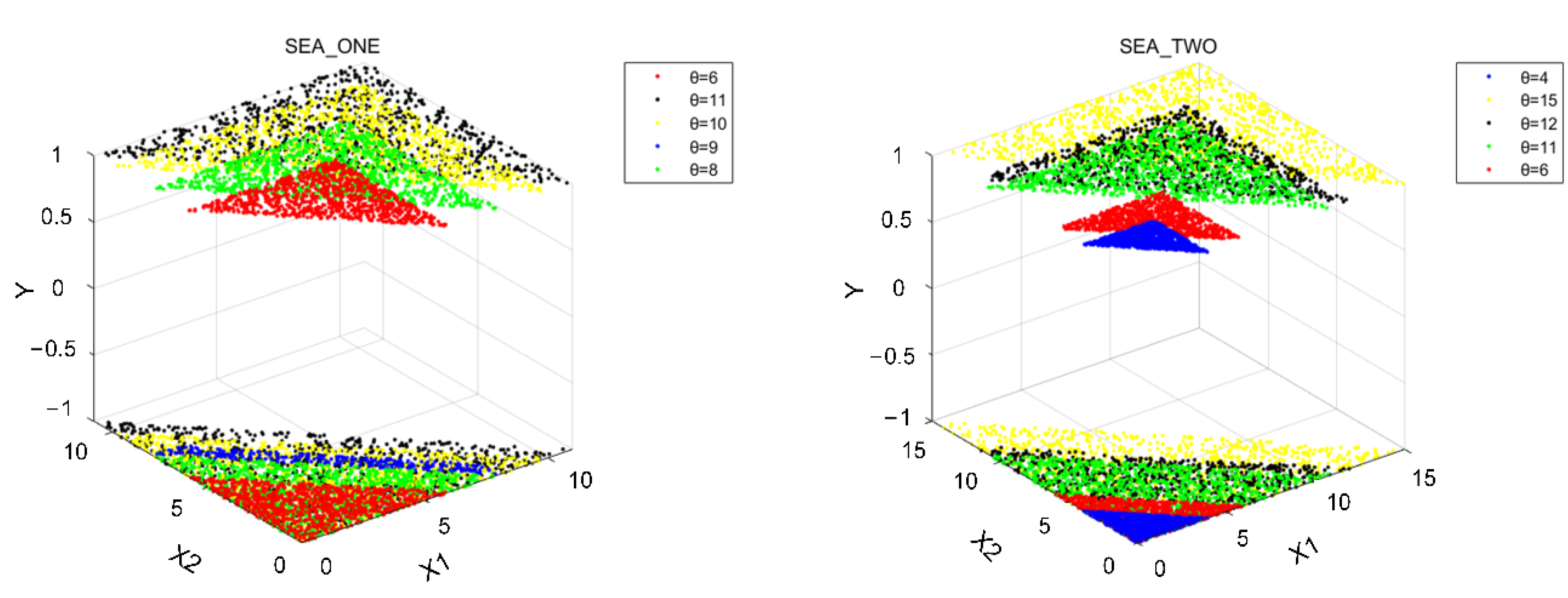
4.1.2. Synthetic Data

Since we cannot obtain real data distribution, synthetic data are used to compare the performance of different types and degrees of concept drift. We selected two additional concept data, SEA (streaming ensemble algorithm), moving hyperplane concepts, and CIR (circle) concepts.

• SEA moving hyperplane concepts [21] have three features $x_1$, $x_2$, and $x_3$. Their value is between 0 and 10. Feature $x_1$ and feature $x_2$ are relevant, while $x_3$ is a noisy feature with a random value. The class label of data in this concept is determined by Equation (17).

$$a{x}_1+b{x}_2\le />\theta$$

(17)

To simulate the concept drift, set different values of $\theta$.

2.

CIR concepts [21] apply a circle as the decision boundary in a 2-D feature space. To simulate the concept drift, we set a different radius of the circle, that is, Equation (18).

$${\left(x_1-a\right)}^2+{\left(x_2-b\right)}^2\le />\theta$$

(18)

In the experiment, each dataset is divided into two parts according to the degree of concept drift. SEA_ONE and CIR_ONE have a small changing degree, while SEA_TWO and CIR_TWO have a great changing degree. Under these conditions, each dataset was randomly generated. The result is shown in Table 3.

Table 3. Concept drift of synthetic data.

Drift Type	Fixed-Parameter	Drift Rate	Drift Parameter
SEA_ONE	A = 1, b = 1	Low	$\theta$ = 10, 8, 6, 9, 11
SEA_TWO		High	$\theta$ = 12, 6, 11, 4, 15
CIR_ONE	A = 0, b = 0	Low	$\theta$ = 3, 2, 1, 4, 6
CIR_TWO		High	$\theta$ = 1, 6, 2, 7, 3

The difference in distribution between SEA_ONE and SEA_TWO is shown in Figure 1. For SEA_ONE, θ is 10, 8, 6, 9, 11 in turn, while for SEA_TWO, θ is 12, 6, 11, 4, 15. It can be seen that the dataset in SEA_ONE is closer than the dataset in SEA_TWO.

Figure 1. Concept distribution of SEA_ONE and SEA_TWO with different $\theta$.

The difference in distribution between CIR_ONE and CIR_TWO is shown in Figure 2. For CIR_ONE, θ is 3, 2, 1, 4, 6 in turn, and for CIR_TWO, θ is 1, 6, 2, 7, 3 in turn. It can be seen that the dataset in CIR_ONE is closer than the dataset in CIR_TWO.

Figure 2. Concept distribution of CIR_ONE and CIR_TWO with different $\theta$.

4.2. Result Analysis

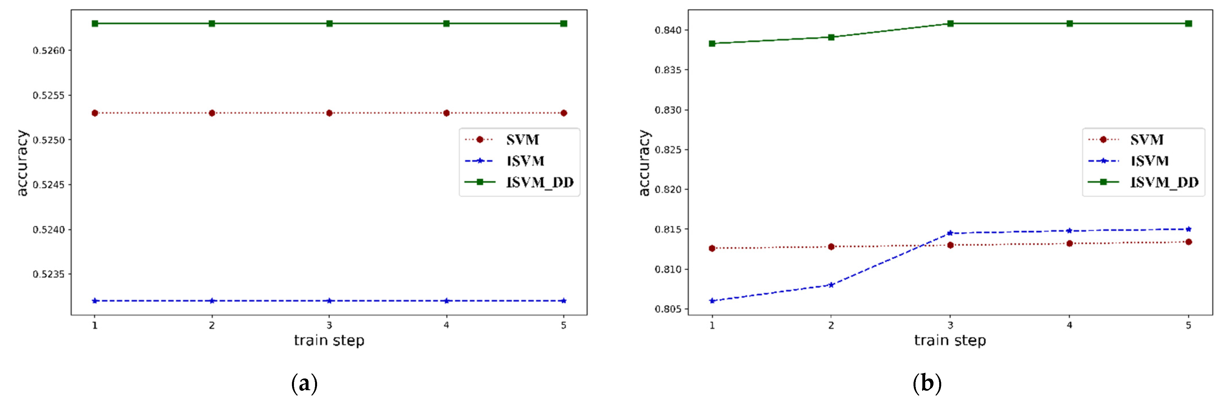
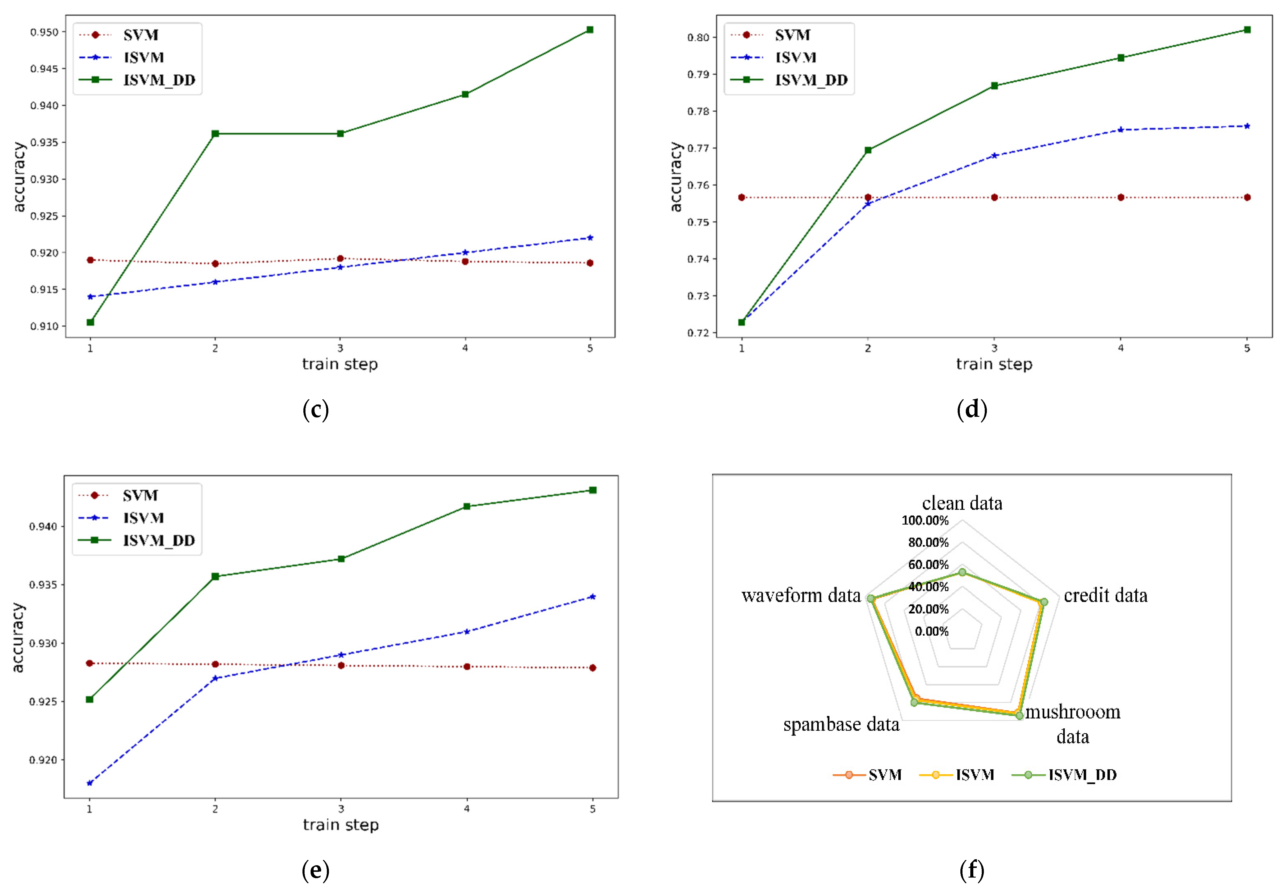
4.2.1. Results on Real Data

Catastrophic forgetting is a critical standard for judging an incremental learning algorithm. If catastrophic forgetting occurs, the incremental learning algorithm cannot maintain previous knowledge, which means it is not learning incrementally.

In this experiment, we randomly divide the experimental data into a training set and a test set, of which 90% is the training set and 10% is the test set. The data of the training set are randomly divided into five subsets, S1–S5, which are added to the model incrementally.

In this experiment, we test the performance of the model on both new data and previous data after each fine-tuning of the model on new data. The training and testing results of the proposed ISVM_DD algorithm on five datasets are shown in Table 4, Table 5, Table 6, Table 7 and Table 8. Train 1 represents the model training. Train 2, train 3, train 4, and train 5 represent the fine-tuning of the model on new data S2, S3, S4, and S5.

Table 4. Result of ISVM_DD on clean data.

Dataset	Accuracy on Clean Data (%)
	Train 1	Train 2	Train 3	Train 4	Train 5
S1	57.89%	57.89%	57.89%	57.89%	57.89%
S2	—	60.00%	60.00%	60.00%	60.00%
S3	—	—	56.84%	56.84%	56.84%
S4	—	—	—	62.10%	62.10%
S5	—	—	—	—	67.36%

Table 5. Result of ISVM_DD on credit data.

Dataset	Accuracy on Credit Data (%)
	Train 1	Train 2	Train 3	Train 4	Train 5
S1	86.08%	85.91%	86.08%	85.75%	86.08%
S2	—	83.50%	83.16%	82.91%	83.16%
S3	—	—	86.16%	85.75%	85.75%
S4	—	—	—	83.25%	82.41%
S5	—	—	—	—	84.33%
Test	83.83%	83.91%	84.08%	84.08%	84.08%

Table 6. Result of ISVM_DD on mushroom data.

Dataset	Accuracy on Mushroom Data (%)
	Train 1	Train 2	Train 3	Train 4	Train 5
S1	95.12%	91.58%	93.44%	93.17%	93.17%
S2	—	92.02%	92.55%	91.93%	91.93%
S3	—	—	93.35%	92.64%	92.64%
S4	—	—	—	93.35%	92.64%
S5	—	—	—	—	95.21%
Test	91.05%	93.62%	93.62%	94.15%	95.03%

Table 7. Result of ISVM_DD on spambase data.

Dataset	Accuracy on Spambase Data (%)
	Train 1	Train 2	Train 3	Train 4	Train 5
S1	83.58%	76.30%	81.41%	77.71%	80.65%
S2	—	85.97%	83.80%	78.26%	82.17%
S3	—	—	85.43%	76.30%	80.43%
S4	—	—	—	83.69%	82.17%
S5	—	—	—	—	86.41%
Test	72.28%	76.95%	78.69%	79.45%	80.21%

Table 8. Result of ISVM_DD waveform data.

Dataset	Accuracy on Waveform Data (%)
	Train 1	Train 2	Train 3	Train 4	Train 5
S1	92.67%	90.58%	91.33%	90.88%	92.22%
S2	—	93.57%	93.57%	93.42%	94.31%
S3	—	—	91.18%	91.77%	92.97%
S4	—	—	—	93.87%	93.27%
S5	—	—	—	—	93.27%
Test	92.52%	93.57%	93.72%	94.17%	94.31%

The first row of Table 4 shows the classification accuracy of the five models on the first dataset, S1. It can be seen that from model1 to model5, the classification accuracy of S1 is consistent, which means there is no catastrophic forgetting of information. The last row shows the test accuracy of the model on the latest dataset after each fine-tuning. It can be seen that each model can achieve good accuracy on the test set of the latest dataset, which means the model has learned new information after fine-tuning.

It can be seen from S1 in Table 4 that the training accuracy from training 1 to training 5 keeps stable, which means there is no catastrophic forgetting of information. Similarly, there is no catastrophic forgetting of information for other subsets from Table 4 to Table 8. The knowledge learned from the old dataset is not forgotten when learning new datasets.

Table 4, Table 5, Table 6, Table 7 and Table 8 show that with the input data (S1, S2, S3, S4, and S5 ) arriving and learning new datasets, the accuracy of the test set is gradually improving, which means it can learn new knowledge from new datasets. This also proves that as the training increases, more knowledge is learned.

Combining the above two points, the proposed ISVM_DD algorithm can learn new knowledge without forgetting the knowledge learned from the old data. In other words, the proposed ISVM_DD algorithm can learn incrementally.

The first row of Table 5, Table 6, Table 7 and Table 8 also shows the classification accuracy of the five models on the first dataset, S1. It can be seen that from model1 to model5, the classification accuracy of S1 fluctuates a little, but there is no significant decrease, which means there is no catastrophic forgetting of information. Fluctuations in model performance may be due to concept drift in these four datasets. The last row shows the test accuracy of the model on the latest dataset after each fine-tuning. It can be seen that each model can achieve good accuracy on the test set of the latest dataset, which means the model has learned new information after fine-tuning.

The result in Table 4, Table 5, Table 6, Table 7 and Table 8 shows the knowledge learned from the old dataset is not forgotten when learning new datasets. With the input data arriving and learning from new datasets, the test accuracy is improving gradually, which means it can learn new knowledge from new datasets. This also proves that as the training increases, more knowledge is learned.

The average test accuracy of SVM, ISVM, and ISVM_DD on five datasets is also compared, and the result is shown in Figure 3 and Table 9.

Figure 3. Comparison of the average test accuracy on five real datasets and the radar chart. (a) is clean data, (b) is credit data, (c) is mushroom data, (d) is spambase data, (e) is waveform data, and (f) is radar charts on five datasets.

Table 9. Result of algorithms on five datasets.

Algorithm	Test Accuracy (%)
	Clean Data	Credit Data	Mushroom Data	Spambase Data	Waveform Data
SVM	52.53%	81.34%	91.86%	75.67%	92.79%
ISVM	52.32%	81.52%	92.23%	77.38%	93.42%
ISVM_DD	52.63%	84.08%	95.03%	80.21%	94.31%

It shows that ISVM_DD gains performance improvements of about 3% on 4 out of 5 datasets. It means incremental learning could perform better when data has concept drift than batch learning. The comparison between ISVM and ISVM_DD shows that domain adaptation could decrease concept drift.

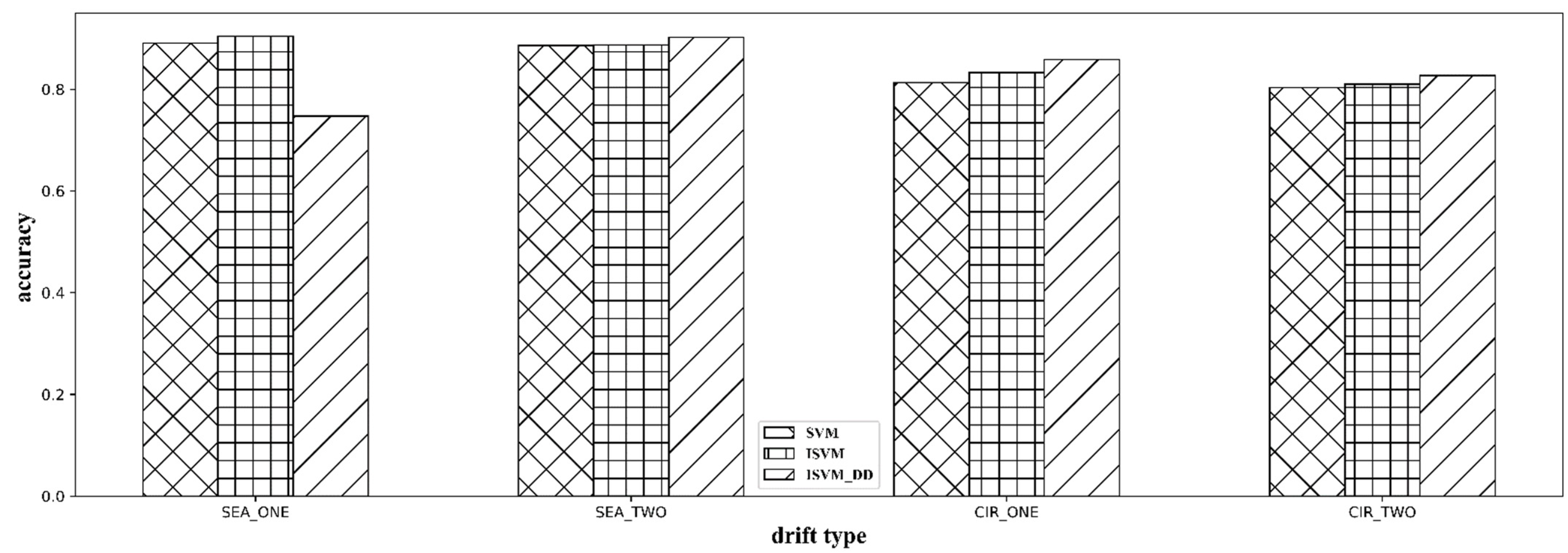
4.2.2. Results on Synthetic Data

From the results of real data, the performance of different datasets differs. It is somewhat related to the type and changing rate of concept drift. However, the type and changing rate of concept drift in real data could not be known, so two synthetic datasets are used to investigate the influence of concept drift type and changing rate.

There are two kinds of concept drift: SEA moving hyperplane concepts and circle concepts, and the corresponding datasets are SEA and CIR. Each dataset is divided into two parts according to the changing rate of concept drift. SEA_ONE and CIR_ONE have low changing rates, while SEA_TWO and CIR_TWO have high changing rates. The result is shown in Table 10 and Figure 4.

Table 10. The average accuracy of different types and different degrees of concept drift.

Algorithm	SEA_ONE	SEA_TWO	CIR_ONE	CIR_TWO
SVM	89.07%	88.65%	81.33%	80.32%
ISVM	90.46%	88.74%	83.27%	81.03%
ISVM_DD	94.77%	90.24%	84.88%	82.69%

Figure 4. Performance comparison of ISVM_DD on datasets with different types and degrees of concept drift.

Table 10 shows that for different concept drifts, all these three algorithms show different performances, and ISVM_DD performs better than SVM and ISVM on all four datasets. However, for concept drift with a high changing rate, ISVM and ISVM_DD decrease average accuracy.

Figure 4 shows that for different types of concept drift, such as SEA and CIR, the algorithm ISVM-DD shows a similar difference. However, for different drift degrees, it offers significantly different performance. Figure 4 shows a slight drift degree, and the algorithm shows good performance, while for a great drift degree, the performance has an obvious decrease. When the drift degree is great, the distance between two concepts is so significant that one adaptation is not enough to connect them.

5. Conclusions

Incremental learning is an effective approach to addressing increasing and changing data. However, concept drift is still a crucial problem limiting incremental learning. In this paper, to decrease the effect of concept drift in incremental learning, we proposed an ISVM_DD algorithm. On the one hand, the proposed ISVM_DD is able to acquire new knowledge from newly added training data while retaining the knowledge learned before without catastrophic forgetting through domain adaptation. On the other hand, by the model selection, the proposed ISVM_DD can forget obsolete information without corrupting still valid, already learned information. The experiment indicates the ISVM_DD achieve better performance compared to previous algorithms.

Furthermore, we studied the effect of the type and degree of concept drift on ISVM_DD. We found that the type and changing rate of concept drift will affect the performance, especially the degree. When dramatic concept drift occurs, the performance of ISVM_DD will decrease. It may be because just once domain adaptation could not connect the source domain and target domain, which is called a transitive transfer learning problem [48]. In the future, we will investigate multiple domain adaptation among some intermediate domains to decrease dramatic concept drift.

References

1. Polikar, R.; Upda, L.; Upda, S.S. Learn++: An incremental learning algorithm for supervised neural networks. IEEE Trans. Syst. Man Cybern. Part C 2001, 31, 497–508. [Google Scholar] [CrossRef]
2. Yu, H.; Lu, J.; Zhang, G. An online robust support vector regression for data streams. IEEE Trans. Knowl. Data Eng. 2020, 34, 150–163. [Google Scholar] [CrossRef]
3. Gâlmeanu, H.; Andonie, R. Weighted Incremental-Decremental Support Vector Machines for concept drift with shifting window. Neural Netw. 2022, 152, 528–541. [Google Scholar] [CrossRef] [PubMed]
4. Muhlbaier, M.; Topalis, A.; Polikar, R. Incremental learning from unbalanced data. In Proceedings of the IEEE International Joint Conference on Neural Networks 2004, Budapest, Hungary, 25–29 July 2004; Volume 2, pp. 1057–1062. [Google Scholar]
5. Muhlbaier, M.; Topalis, A.; Polikar, R. Learn++. MT: A New Approach to Incremental Learning. In Proceedings of the Springer International Workshop on Multiple Classifier Systems; Springer: Berlin/Heidelberg, Germany, 2004; pp. 52–61. [Google Scholar]
6. Mohammed, H.S.; Leander, J.; Marbach, M. Comparison of Ensemble Techniques for Incremental Learning of New Concept Classes under Hostile Non-stationary Environments. In Proceedings of the IEEE International Conference on Systems, Man and Cybernetics, Taipei, Taiwan, 8–11 October 2006; pp. 4838–4844. [Google Scholar]
7. Elwell, R.; Polikar, R. Incremental learning in non-stationary environments with controlled forgetting. In Proceedings of the IEEE International Joint Conference on Neural Networks, Atlanta, GA, USA, 14–19 June 2009; pp. 771–778. [Google Scholar]
8. Uhlbaier, M.D.; Topalis, A.; Polikar, R. Learn++. NC: Combining Ensemble of Classifiers With Dynamically Weighted Consult-and-Vote for Efficient Incremental Learning of New Classes. IEEE Trans. Neural Netw. 2009, 20, 152–168. [Google Scholar] [CrossRef]
9. Karnick, M.; Muhlbaier, M.D.; Polikar, R. Incremental learning in non-stationary environments with concept drift using a multiple classifier-based approach. In Proceedings of the IEEE International Conference on Pattern Recognition, Tampa, FL, USA, 8–11 December 2008; pp. 1–4. [Google Scholar]
10. Elwell, R.; Polikar, R. Incremental Learning of Variable Rate Concept Drift. In Proceedings of the International Workshop on Multiple Classifier Systems; Springer: Berlin/Heidelberg, Germany, 2009; pp. 142–151. [Google Scholar]
11. Ditzler, G.; Polikar, R. An ensemble based incremental learning framework for concept drift and class imbalance. In Proceedings of the IEEE International Joint Conference on Neural Networks, Barcelona, Spain, 18–23 July 2010; pp. 1–8. [Google Scholar]
12. Dong, X.; Yu, Z.; Cao, W.; Shi, Y.; Ma, Q. A survey on ensemble learning. Front. Comput. Sci. 2020, 14, 241–258. [Google Scholar] [CrossRef]
13. Sagi, O.; Rokach, L. Ensemble learning: A survey. Wiley Interdiscip. Rev. 68p25 Knowl. Discov. 2018, 8, e1249. [Google Scholar] [CrossRef]
14. Wang, Y.; Zhang, F.; Chen, L. An Approach to Incremental SVM Learning Algorithm. In Proceedings of the IEEE International Colloquium on Computing, Communication, Control, and Management, Guangzhou, China, 3–4 August 2008; pp. 352–354. [Google Scholar]
15. Liang, Z.; Li, Y.F. Incremental support vector machine learning in the primal and applications. Neurocomputing 2009, 72, 2249–2258. [Google Scholar] [CrossRef]
16. Zheng, J.; Shen, F.; Fan, H.; Zhao, J. An online incremental learning support vector machine for large-scale data. Neural Comput. Appl. 2013, 22, 1023–1035. [Google Scholar] [CrossRef]
17. Wang, J.; Yang, D.; Jiang, W.; Zhou, J. Semisupervised incremental support vector machine learning based on neighborhood kernel estimation. IEEE Trans. Syst. Man Cybern. Syst. 2017, 47, 2677–2687. [Google Scholar] [CrossRef]
18. Gu, B.; Quan, X.; Gu, Y.; Sheng, V.S.; Zheng, G. Chunk incremental learning for cost-sensitive hinge loss support vector machine. Pattern Recognit. 2018, 83, 196–208. [Google Scholar] [CrossRef]
19. Li, J.; Dai, Q.; Ye, R. A novel double incremental learning algorithm for time series prediction. Neural Comput. Appl. 2019, 31, 6055–6077. [Google Scholar] [CrossRef]
20. Aldana, Y.R.; Reyes, E.J.M.; Macias, F.S.; Rodríguez, V.R.; Chacón, L.M.; Van Huffel, S.; Hunyadi, B. Nonconvulsive epileptic seizure monitoring with incremental learning. Comput. Biol. Med. 2019, 114, 103434. [Google Scholar] [CrossRef] [PubMed]
21. Li, Y.; Wang, Y.; Liu, Q.; Bi, C.; Jiang, X.; Sun, S. Incremental semi-supervised learning on streaming data. Pattern Recognit. 2019, 88, 383–396. [Google Scholar] [CrossRef]
22. Hu, J.; Li, T.; Luo, C.; Fujita, H.; Yang, Y. Incremental fuzzy cluster ensemble learning based on rough set theory. Knowl.-Based Syst. 2017, 132, 144–155. [Google Scholar] [CrossRef]
23. Pari, R.; Sandhya, M.; Sankar, S. A Multi-Tier Stacked Ensemble Algorithm to Reduce the Regret of Incremental Learning for Streaming Data. IEEE Access 2018, 6, 48726–48739. [Google Scholar] [CrossRef]
24. Jiménez-Guarneros, M.; Alejo-Eleuterio, R. A Class-Incremental Learning Method Based on Preserving the Learned Feature Space for EEG-Based Emotion Recognition. Mathematics 2022, 10, 598. [Google Scholar] [CrossRef]
25. Widmer, G.; Kubat, M. Learning in the presence of concept drift and hidden contexts. Mach. Learn. 1996, 23, 69–101. [Google Scholar] [CrossRef]
26. Hulten, G.; Spencer, L.; Domingos, P. Mining time-changing data streams. In Proceedings of the Seventh ACM SIGKDD International Conference on Knowledge Discovery and Data Mining, ACM, San Francisco, CA, USA, 26–29 August 2001; pp. 97–106. [Google Scholar]
27. Zhu, Q.; Hu, X.; Zhang, Y.; Li, P.; Wu, X. A double-window-based classification algorithm for concept drifting data streams. In Proceedings of the IEEE International Conference on Granular Computing, San Jose, CA, USA, 14–16 August 2010; pp. 639–644. [Google Scholar]
28. Bifet, A.; Gavalda, R. Learning from time-changing data with adaptive windowing. In Proceedings of the 2007 SIAM International Conference on Data Mining, Minneapolis, MN, USA, 26–28 April 2007; Society for Industrial and Applied Mathematics. pp. 443–448. [Google Scholar]
29. Núñez, M.; Fidalgo, R.; Morales, R. Learning in environments with unknown dynamics: Towards more robust concept learners. J. Mach. Learn. Res. 2007, 8, 2595–2628. [Google Scholar]
30. Chen, C.; Xie, W.; Huang, W.; Rong, Y.; Ding, X.; Huang, Y.; Huang, J. Progressive Feature Alignment for Unsupervised Domain Adaptation. In Proceedings of the IEEE Conference on Computer Vision and Pattern Recognition, Long Beach, CA, USA, 16–20 June 2019. [Google Scholar]
31. Chen, Y.; Yang, C.L.; Zhang, Y.; Li, Y.Z. Deep conditional adaptation networks and label correlation transfer for unsupervised domain adaptation. Pattern Recognit. 2020, 98, 107072. [Google Scholar] [CrossRef]
32. He, T.; Shen, C.; Tian, Z.; Gong, D.; Sun, C.; Yan, Y. Knowledge Adaptation for Efficient Semantic Segmentation. In Proceedings of the IEEE Conference on Computer Vision and Pattern Recognition, Long Beach, CA, USA, 16–20 June 2019. [Google Scholar]
33. Huang, J.; Smola, A.J.; Gretton, A.; Borgwardt, K.M.; Schölkopf, B. Correcting sample selection bias by unlabeled data. In Proceedings of the NIPS, Barcelona, Spain, 9 December 2016. [Google Scholar]
34. Vapnik, V.; Izmailov, R. Knowledge transfer in SVM and neural networks. Ann. Math. Artif. Intell. 2017, 81, 3–19. [Google Scholar] [CrossRef]
35. Pan, S.J.; Yang, Q. A survey on transfer learning. IEEE Trans. Knowl. Data Eng. 2009, 22, 1345–1359. [Google Scholar] [CrossRef]
36. Farahani, A.; Voghoei, S.; Rasheed, K.; Arabnia, H.R. A brief review of domain adaptation. In Proceedings of the International Conference on Data Science, Las Vegas, NV, USA, 27–30 July 2020; pp. 877–894. [Google Scholar]
37. Kemker, R.; McClure, M.; Abitino, A.; Hayes, T.; Kanan, C. Measuring catastrophic forgetting in neural networks. In Proceedings of the AAAI Conference on Artificial Intelligence, New Orleans, LA, USA, 2–7 February 2018. [Google Scholar]
38. Nadira, A.; Abdessamad, A.; Mohamed, B.S. Regularized Jacobi Wavelets Kernel for Support Vector Machines. Statistics. Opti-Misation Inf. Comput. 2019, 7, 669–685. [Google Scholar]
39. Cortes, C.; Vapnik, V. Support vector machine. Mach. Learn. 1995, 20, 273–297. [Google Scholar] [CrossRef]
40. Wu, Y.; Ma, X. Alarms-related wind turbine fault detection based on kernel support vector machines. J. Eng. 2019, 18, 4980–4985. [Google Scholar] [CrossRef]
41. Xu, J.; Xu, C.; Zou, B. New Incremental Learning Algorithm with Support Vector Machines. IEEE Trans. Syst. Man Cybern. Syst. 2018, 99, 1–12. [Google Scholar] [CrossRef]
42. Zhang, Z.; Wang, M.; Nehorai, A. Optimal Transport in Reproducing Kernel Hilbert Spaces: Theory and Applications. IEEE Trans. Pattern Anal. Mach. Intell. 2019, 42, 1741–1754. [Google Scholar] [CrossRef] [PubMed]
43. Arslan, G.; Madran, U.; Soyoğlu, D. An Algebraic Approach to Clustering and Classification with Support Vector Machines. Mathematics 2022, 10, 128. [Google Scholar] [CrossRef]
44. Liu, X.; Zhao, B.; He, W. Simultaneous Feature Selection and Classification for Data-Adaptive Kernel-Penalized SVM. Mathematics 2020, 8, 1846. [Google Scholar] [CrossRef]
45. Gonzalez-Lima, M.D.; Ludeña, C.C. Using Locality-Sensitive Hashing for SVM Classification of Large Data Sets. Mathematics 2022, 10, 1812. [Google Scholar] [CrossRef]
46. Nalepa, J.; Kawulok, M. Selecting training sets for support vector machines: A review. Artif. Intell. Rev. 2019, 52, 857–900. [Google Scholar] [CrossRef]
47. Moayedi, H.; Hayati, S. Modelling and optimisation of ultimate bearing capacity of strip footing near a slope by soft computing methods. Appl. Soft Comput. 2018, 66, 208–219. [Google Scholar] [CrossRef]
48. Tan, B.; Zhang, Y.; Pan, S.J.; Yang, Q. Distant domain transfer learning. In Proceedings of the Thirty-First AAAI Conference on Artificial Intelligence, San Francisco, CA, USA, 4–9 February 2017. [Google Scholar]
Publisher’s Note: MDPI stays neutral with regard to jurisdictional claims in published maps and institutional affiliations.
Article Metrics
Citations
Article Access Statistics
Multiple requests from the same IP address are counted as one view.