Reachset Conformance and Automatic Model Adaptation for Hybrid Systems

Abstract

Model-based verification uses a model to reason about the correctness of a real system. This requires the model and the system to be conformant, such that verification results on the model can be transfered to the real system. Especially for hybrid systems, which combine discrete and continuous behavior, defining and checking conformance is a difficult task. In this work, we present reachset conformance for hybrid systems that transfers safety properties from a model to the real system. We show how a model can be adapted to be conformant to measurements of a real system and demonstrate this for a real autonomous vehicle. The obtained reachset conformant model can be used for the verification of safety-critical properties, such as collision avoidance.

1. Introduction

The amount of technical systems operating autonomously and without human interference is continuously growing. It is of utmost importance to demonstrate that such autonomous systems cannot harm people, cause damage, or breach any other important specification. Autonomous vehicles and moving robots are examples of such safety-critical applications, where the discrete and continuous aspects are tightly intertwined—these systems are often referred to as hybrid systems.

Model-based formal verification is an important approach toward safer systems. In particular, reachability analysis computes the set of reachable states of a model and can be used to check whether unsafe states are possible [1,2]. To include different possible behaviors of the real system, verification models for reachability analysis are non-deterministic. This means that at each point in time, there might be multiple evolutions of the model, and one has to reason about all of them. The basic assumption of model-based verification is that the model is related to the system in a way that the safety of the system can be implied if the safety of the model has been shown. We call a relation between a system and a model conformance relation and argue that it should also be defined formally. Otherwise, one cannot be sure that the used conformance relation allows to transfer safety properties from the model to the real system, which would make the formal verification effort useless. Hence, the conformance relation connects the formal world of reasoning with the real world.

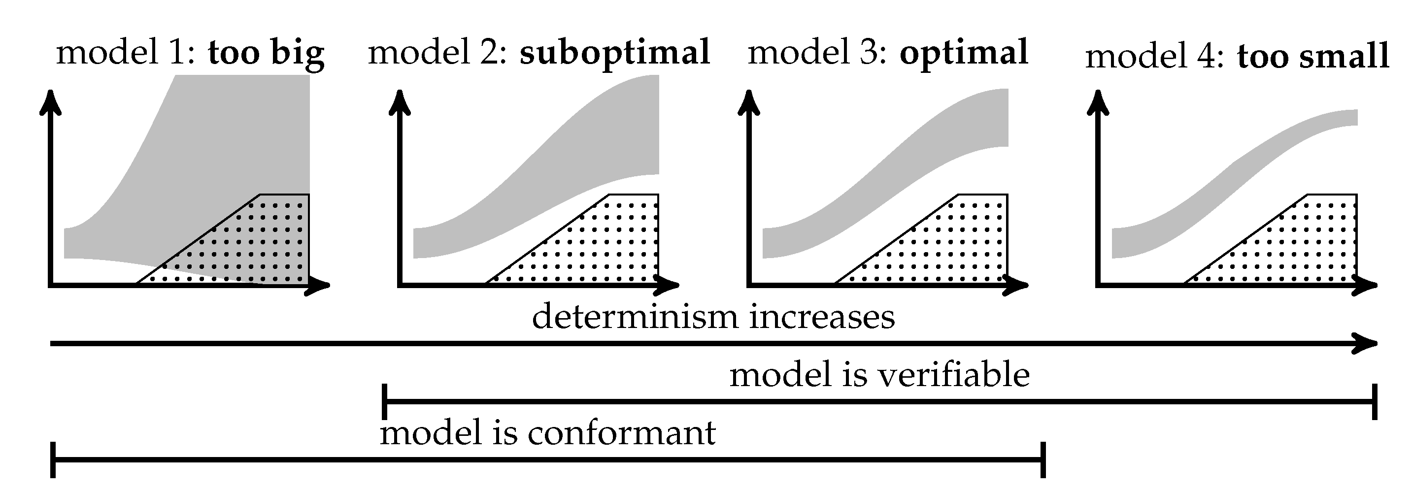
A major challenge of a verification model is that it simultaneously has to be amenable to verification and conformance. This is challenging because (i) a model with significant non-determinism is conformant, but it might have too many reachable states to verify properties (model 1 in Figure 1) and (ii) a model with insignificant non-determinism is amenable for verification, but it might not be conformant to the real system because some states cannot be produced by the model (model 4 in Figure 1). Between these two extremes are the most useful models, amenable for both verification and conformance (model 2 and model 3 in Figure 1). We argue that an optimal model has just enough non-determinism such that reachset conformance holds to sustain the most freedom possible for verification. A method is needed to build verification models maximizing verification capabilities while ensuring conformance.

In a previous paper [3], we introduced reachset conformance and showed how to test it for a given (hybrid-system) model M and measurements of a (real) system S. Here, we extend these results in several aspects:

Natural choice: We show that safety properties can be transfered from M to S exactly in the case when reachset conformance between M and S holds. Therefore, reachset conformance is the natural choice to transfer safety properties.

Quantified reachset conformance check: A robustness measure is introduced, which is based on the distance of a point to the boundary of a reachable set. In our setting, reachable sets are represented as zonotopes, and as a result, exclusion can be checked using linear programming techniques. This is computed for the measured data of the real system of some input and the output of the verification model for the same input, cf. Figure 2.

Model adaptation: We show how to automatically adapt the non-determinism of a model M, such that M becomes reachset-conformant to S. This is computed by identifying bounds on non-deterministic parameters. The bounds are optimized using Bayesian optimization to minimize the non-determinism while being conformant, Figure 1. In addition to building a reachset-conformant model, the method maximizes the verification capabilities of the model, cf. model 3 in Figure 2. Thus, our method helps to overcome the burden of building a formal verification model.

Autonomous vehicle application: We apply our methods to a real automated vehicle and construct a verification model of the vehicle. Measured driving data of the automated vehicle were recorded, and our model adaptation was applied to identify the non-determinism of the verification model such that the model is reachset-conformant to the automated vehicle. Our verification model is amenable to verification, showing that our approach is applicable to the highly relevant use case of autonomous vehicles. This is the first work showing reachset conformance for a real (autonomous) vehicle.

The paper is structured as follows: First, we discuss related work on conformance and verification in Section 2. In Section 3, we present the underlying formalism of hybrid automata and other preliminaries. In Section 4, we present reachset conformance, prove that it is necessary and sufficient to transfer safety properties, and compare it to trace conformance, which is discussed in [4]. In Section 5, we present a testing method for reachset conformance. In Section 6, we introduce our model adaptation algorithm. In Section 7, we apply the presented techniques to a real vehicle and build a reachset-conformant vehicle model. Finally, we give some conclusions and future directions.

2. Related Work

2.1. Verification

An overview of safety verification for hybrid systems is provided by Guéguen et al. [1]. Schupp et al. [5] give an overview of methods for the reachability analysis of hybrid systems and discuss their challenges with respect to verification. In this work, we focus on reachability-based verification techniques. In the context of our application example autonomous vehicles, the reachability analysis tool CORA [6] has been used for the verification of cooperative and non-cooperative maneuvers of autonomous vehicles [7]. The reachability analysis computations are fast enough to allow online verification while the vehicle is driving [7].

2.2. Conformance

A variety of conformance relations have been defined. For brevity, we are only mentioning the most important ones here and refer to the survey by Roehm et al. [8] for a detailed overview of different conformance relations. Since properties are typically specified on output traces, one important notion of conformance is the trace conformance for hybrid automata [4] and similarly hybrid input–output conformance [9]. It requires that all possible output traces of one system S are also output traces of the other system M. Trace conformance reflects the conventional notion of conformance of discrete automata where traces of one system also have to be traces of the other one [10]. When trace conformance holds, universally quantified properties are transfered, such as metric temporal logic formulas [11].

Trace conformance has been generalized to approximate versions, which do not require the traces of one system to be included in the other but allow some deviation. The $(\tau ,\epsilon )$-closeness [12] allows for some value-differences as well as time-shifts. $(\tau ,\epsilon )$-closeness testing is performed by using a robustness value as a heuristic to guide the testing to non-conformant behavior [13]. $\epsilon$-$\delta$-similarity is a similar notion to $(\tau ,\epsilon )$-closeness but does not allow local time disorder in the comparison of two traces [14]. The $\epsilon$-Skorokhod conformance [15] uses the Skorokhod metric to quantify the distance between traces. The Skorokhod distance can be also computed between reachpipes [16], which are for instance traces with an $\epsilon$-ball around them. One problem is that approximate relations do not transfer properties directly, but the property alters on transference [11,15].

So far, we only reviewed conformance relations applied to the output space. On the contrary, there are a variety of other conformance relations relating states of the systems which are called simulation relations [17,18,19,20,21,22]. The basic idea is that states of both systems are related such that evolutions from any state of one system can be mirrored by evolutions of a related state of the other system. There also exist approximative versions of simulation relations, which require the states to just be approximately similar [23,24,25]. On one hand, simulation relations transfer more properties compared to trace conformance. On the other hand, they require the systems to be more similar to each other than trace conformance. Since simulation relations require knowledge of the states, real systems cannot be considered since their exact state is unaccessible, except when all states can be measured. Hence, we will focus on comparing the reachset conformance relation to trace conformance (cf. Section 4). For a discussion between simulation relation and reachset conformance, we refer to the survey by Roehm et al. [8].

While we have introduced reachset conformance in 2016 [3], there is already some work in the direction of identification of non-determinism for reachset conformance. Liu and Althoff [26] have published a method to identify non-determinism for dynamical systems to be reachset conformant and applied it to the reachset conformance of robots. Kochdumper et al. [27] have shown a synthesis algorithm for the reachset conformance of linear hybrid systems leveraging the internal structure of the hybrid system. Furthermore, methods to bound additive errors for discrete-time dynamical models have been published [28,29]. Contrary to these methods, our method does not require any special knowledge on the hybrid system and is not restricted to a subclass of hybrid systems.

There exist methods for finding the parameters of a deterministic hybrid system to approximate measured data [30]. Our work differ in that we are identifying the non-determinism needed to include measurements in a non-deterministic model.

3. Preliminaries

In this paper, we use hybrid automata as a modeling formalism. A hybrid automaton can be seen as a finite automaton whose discrete states are annotated with differential inclusions that define the non-deterministic evolution of the continuous states [31]. An overview of definitions of hybrid automata and their differences has been presented by Frehse [17]. In our work, a (non-deterministic) hybrid automaton H consists of

• A finite set of locations $Q\subset \mathbb{N}$;
• A continuous state space $X\subseteq {\mathbb{R}}^n$;
• An initial set $I_H\subseteq Q\times X$;
• A continuous input space $U\subseteq {\mathbb{R}}^m$;
• A flow function $F_H:Q\times X\times U\to \mathcal{P}\left(X\right)$, where $\mathcal{P}\left(X\right)$ is the power set of X;
• An invariant set $inv\left(q\right)\subseteq X$ for each location q;
• A set of discrete transitions $\mathcal{T}\subseteq Q\times Q$;
• A guard set $guard\left((q,q^{\prime })\right)$ for each transition $(q,q^{\prime })\in \mathcal{T}$;
• A jump function $jum{p}_{(q,q^{\prime })}:X\to \mathcal{P}\left(X\right)$ for each transition $(q,q^{\prime })\in \mathcal{T}$;
• An output space $O\subseteq {\mathbb{R}}^l$;
• An output map $out:Q\times X\to O$.

For a given input function $u:{\mathbb{R}}^{+}\to U$, which maps each point in time to an input value, a state trace x of H is

$$x=(q_0,x_0(.))(q_1,x_1(.))\dots$$

(1)

with discrete states $q_i\in Q$, continuous state functions $x_i:[t_i,t_{i+1}]\to X$, and with the initial state $(q_0,x_0\left(0\right))\in I_H$. The transitions from $q_i$ to a new state $q_{i+1}$ have to satisfy $(q_i,q_{i+1})\in \mathcal{T}$. The continuous state function $x_i(.)$ has to satisfy the invariant set $x_i\left(t\right)\in inv\left(q_i\right)$ and the differential inclusion ${\dot{x}}_i\left(t\right)\in F_H(q_i,x_i\left(t\right),u\left(t\right))$. Upon a discrete transition $(q_i,q_{i+1})$, the continuous state satisfies $x_i\left(t_{i+1}\right)\in guard\left((q_i,q_{i+1})\right)$ as well as $x_{i+1}\left(t_{i+1}\right)\in jum{p}_{(q_i,q_{i+1})}\left(x_i\left(t_{i+1}\right)\right)$. Note that we have a non-deterministic initial state, non-deterministic flow and jump functions, so there are multiple state traces possible for a given input trajectory $u(.)$. The set of state traces for a given hybrid automaton H with initial set $I_H$ under input $u(.)$ is denoted by $straces(H,u(.),I_H)$.

While state traces represent the internal states of the system, they are not observable. Instead, we are able to observe the output trace $\tau :{\mathbb{R}}^{+}\to O$ which is the mapping of the state trace x onto the observable output space via the map $out$:

$$\forall i\forall t\in [t_i,t_{i+1}):\tau \left(t\right)=out(q_i,x_i\left(t\right)).$$

(2)

The set of all output traces under an input trajectory $u(.)$ and the initial set $I_H$ is denoted by $otraces(H,u(.),I_H)$. Therefore, the set $otraces(H,u(.),I_H)$ represents all possible observable behaviors over time for the given $u(.)$ and $I_H$. If $otraces(H,u(.),I_H)$ has one element only for every $u(.)$ and a single initial state, the hybrid automaton H is called deterministic and non-deterministic otherwise.

The already existing trace conformance, which we talked about in the overview section, can now be defined formally:

Definition 1

(trace conformance [4]). Let S and M be two systems with the same input set and output space, and with the initial sets $I_S$ and $I_M$, then S is trace conformant to M, which is denoted by $S{⪯}_{T}M$, if

$$otraces(S,u(.),I_S)\subseteq otraces(M,u(.),I_M)$$

(3)

holds for all $u(.)\in U(.)$.

This means when trace conformance holds, all observable behavior over time of S is also observable of M. A safety property consists of a set of unsafe output states $B_t$ for every time t. If this set is never reachable, i.e.,

$$\forall \tau \in otraces(H,u(.),I_H)\forall t\ge 0:\tau \left(t\right)\notin B_t.$$

(4)

then H is considered safe.

Given such a safety property with $B_t$ and a model M, verification deals with algorithmically checking that (4) holds. When reasoning about the future evolution of a system H, one has to consider all—potentially infinitely many—output traces. With infinitely many traces, dealing with the output traces directly is intractable. One important approach to solve this problem is to use reachability analysis. For one point in time t, the reachable set (or shorter: reachset) of outputs of the hybrid automaton H at time t contains all output states which are possible at time t for a given input trajectory $u(.)$:

$$Reac{h}_t(H,u(.),I_H)=\{\tau \left(t\right)\mid \tau \in otraces(H,u(.),I_H)\}.$$

(5)

We call the sequence of these reachable sets $Reac{h}_t(H,u(.),I_H)$ over time t as the reach sequence of H. Note that the elements of $otraces$ are functions over time, whereas the set $Reac{h}_t$ consists of output states for one point in time t only. Reachable sets can be used to reason about properties of H by verifying that no unsafe set $B_t$ of a safety property is reachable:

$$\forall t\ge 0:Reac{h}_t(H,u(.),I_H)\cap B_t=\varnothing .$$

Since the reach sequence is an abstraction of the output traces $otraces(H,u(.),I_H)$, trace conformance is not the best relation for transference between reach sequences, as described in Section 4. Therefore, we present reachset conformance in the following section.

Let us now more formally and generally specify the problems addressed in this paper. Given a non-deterministic model M of a hybrid system S, the type of relation $S⪯M$ between S and M needed to transfer any safety property $\psi$ from M to S is:

$$S⪯M\wedge M\vDash \psi \Rightarrow S\vDash \psi ,$$

(6)

where $S\vDash \psi$ means system S has the property $\psi$.

Let us also introduce a Gaussian process (Section 6.4, [32]) with parameter vectors $P=(p_1,\dots ,p_n)$ and $V=(v_1,\dots ,v_n)$ as a function $gp$ mapping the input p to a Gaussian distribution with mean $m\left(p\right)$ and variance ${\sigma }^2\left(p\right)$. The $(p_1,v_1)$ are the samples, and the Gaussian process generalizes the mapping by estimating the similarity between different values for p. The functions $m\left(p\right)$ and ${\sigma }^2\left(p\right)$ are defined as [32]:

$$m\left(p\right)=\overline{k}{\left(p\right)}^T{K}^{-1}\overline{c},{\sigma }^2\left(p\right)=k(p,p)-\overline{k}{\left(p\right)}^T{K}^{-1}\overline{k}\left(p\right),$$

(7)

where ${}^T$ is the matrix transposition, and $k(p,p^{\prime })$ is a kernel function defined (in our case) as

$$k(p,p^{\prime }):={\theta }_{0}exp(-{\theta }_1\parallel p-p^{\prime }{\parallel }^2)+{\theta }_2+{\theta }_3{p}^T{p}^{\prime },$$

(8)

$\overline{k}{\left(p\right)}^T=(k(p_1,p),\dots ,k(p_s,p))$, $\overline{c}=(c_1,\dots ,c_s)$, and the matrix K contains the entries $k(p_i,p_j)$ in the $i^{th}$ row and $j^{th}$ column. The parameters ${\theta }_i$ can be computed using hyperparameter optimization with P and V (Section 6.4.2, [32]).

4. Reachset Conformance

With the preliminaries from Section 3, we are now able to formally define the notion of reachset conformance.

Definition 2

(reachset conformance [3]). Let S and M be two systems with the same input space and output space. Let $I_S$ and $I_M$ be the initial sets of S and M, respectively; then, S is reachset-conformant to M, denoted by $S{⪯}_{R}M$, if for all possible inputs $u(.)$ and $t\ge 0$:

$$Reac{h}_t(S,u(.),I_S)\subseteq Reac{h}_t(M,u(.),I_M).$$

(9)

Reachset conformance directly considers the non-determinism of models while still being able to transfer safety properties.

Proposition 1.

Let two systems S and M be given with $S{⪯}_{R}M$ and initial sets $I_S$ and $I_M$, respectively. Let a safety property with forbidden state sets $B_t$ be given for all t. For any input trajectory $u(.)$, the following transference holds for every t:

$$Reac{h}_t(M,u(.),I_M)\cap B_t=\varnothing \Rightarrow Reac{h}_t(S,u(.),I_S)\cap B_t=\varnothing .$$

(10)

Proof. 

Since S is reachset conformant to M and thus $Reac{h}_t(S,u(.),I_S)$ is a subset of $Reac{h}_t(M,u(.),I_M)$ for all t, the proposition follows immediately. □

The following theorem shows that reachset conformance is the natural choice for the transference of safety properties.

Theorem 1.

Let two systems S and M be given. The transference of safety properties is equivalent to reachset conformance: $\left(10\right)\mathit{holds}\mathit{for}\mathit{all}t\mathit{and}\mathit{all}\mathit{possible}{B}_t\iff S{⪯}_{R}M.$

Proof. 

One direction follows from Proposition 1. Let us assume that (10) holds for all t and all possible $B_t$. Choosing $B_t^{\prime }:={\mathbb{R}}^m\setminus Reac{h}_t(M,u(.),I_M)$, which is the complement of the reachable set of M at time t, the intersection of $B_t^{\prime }$ and $Reac{h}_t(M,u(.),I_M)$ is obviously empty. Since this property is transferable from M to S, the equation

$$Reac{h}_t(S,u(.),I_S)\cap ({\mathbb{R}}^m\setminus Reac{h}_t(M,u(.),I_M))=\varnothing$$

holds, and thus, $Reac{h}_t(S,u(.),I_S)\subseteq Reac{h}_t(M,u(.),I_M)$. This works for every t, and thus, S is reachset conformant to M. □

Although we are mainly interested in the transference of safety properties, there are temporal fragments which transfer with reachset conformance. For instance, temporal properties formalizable in reachset temporal logic, which were introduced by Roehm et al. [33]. However, temporal properties cannot be transfered in general, as the reach sequence is an abstraction of the output traces. Reachset conformance is a weaker conformance notion than trace conformance:

Theorem 2.

Let S and M be two systems with the same input set and output space; then,

$$S{⪯}_{T}M\Rightarrow S{⪯}_{R}M$$

(11)

holds. The converse holds if the system M (and thus S) is deterministic.

Proof. 

Let $u(.)$ be an input trajectory, t be a point in time, $y\in Reac{h}_t(S,u(.),I_S)$ and $S{⪯}_{T}M$. Then, there is a $\tau \in otraces(S,u(.),I_S)$ with $\tau \left(t\right)=y$. From $S{⪯}_{T}M$, it follows that $\tau$ is also a trace of M and $y\in Reac{h}_t(M,u(.),I_M)$. The proposition follows, because the aforementioned implication holds for all y, t, and $u(.)$. When the system M is deterministic, there is only one trace in $otraces(M,u(.),I_M)$, and the reachable set for any time consists of only one state. Hence, S has the same trace and is also deterministic. □

This shows that reachset conformance is weaker compared to trace conformance and that we can transfer properties between reachsets in cases where trace conformance does not hold.

5. Reachset Conformance Testing

In this section, we show how to check the reachset conformance of a real system S against a model M. Additionally, we introduce a robustness measure which quantifies conformance. Since proving a physical model against the real world is not possible, the goal is to check if the non-conformance S ${}_R$ M can be shown by a counter-example for a given input $u(.)$. Hence, we have to prove that the negation of (9) holds, which is

$$\exists u(.)\in U(.)\exists t\ge 0:Reac{h}_t(,u(.),I_S)⊈Reac{h}_t(,u(.),I_M).$$

(12)

Our test to check reachset conformance consists of three steps:

1.

Obtain measurements of the system S as an underapproximation $Reac{h}_t^u(,u(.),I_S)\subseteq Reac{h}_t(,u(.),I_S)$ of the reachable states of for a finite set T of points in time $t\in T$.

2.

Compute an overapproximation $Reac{h}_t^o(,u(.),I_M)\supseteq Reac{h}_t(,u(.),I_M)$ of the reachable set of for all $t\in T$.

3.

Check if $Reac{h}_t^u(,u(.),I_S)⊈Reac{h}_t^o(,u(.),I_M)$ holds for any $t\in T$.

If for any t a non-inclusion is found, a counter-example is found, and non-conformance is proven. In the following, we discuss the steps in detail.

5.1. Obtain Measurements of S

Real measurements are subject to noise, and we assume there exists an error $\epsilon$, which bounds the deviation of all measurements $(t_i,{\tau }_i)$ to the true trace $\tau$:

$$\underset{i}{max}{d}_2({\tau }_i-\tau \left(t_i\right))\le \epsilon .$$

(13)

In our case, we consider $d_2(.)$ to be the Euclidean 2-norm. Taking all runs of S for the same input $u(.)$, this approach builds up reachable sets underapproximations.

5.2. Overapproximation of the Reachable Sets of M

An overapproximation of M can be efficiently computed using reachability analysis. Our work builds on the tool CORA [6] to compute reachable set overapproximations for hybrid automata with nonlinear continuous dynamics. CORA uses zonotopes to represent reachable sets due to their efficiency in linear transformations and Minkowski additions [34].

Definition 3

(Zonotope). An n-dimensional zonotope Z in generator representation (G-representation) is the set

$$Z=z(c,\langle g_1,\dots ,g_m\rangle ):=\left\{c+\sum _{i=1}^m{\lambda }_i{g}_i|{\lambda }_i\in [-1,1]\right\},$$

(14)

where $c\in {\mathbb{R}}^n$ is called the center and $g_1,\dots ,g_m\in {\mathbb{R}}^n$ are called the generators of Z.

5.3. Exclusion Check

For a given $t\in T$, we have to check if a given measurement ${\tau }_i$ with $t=t_i$ is excluded from $Reac{h}_t^o(,u(.),I_M)$. Since we consider the measurement error, we have to check that all possible candidates for the real value are not contained to prove exclusion. Hence, the $\epsilon$ ball around ${\tau }_i$ has to be completely outside the reachable set to prove that a counter-example exists.

The distance is important information, which we will use for the model adaptation. Therefore, we are using support functions to define a distance metric (note that the approach using support functions can be applied to other convex (reach-)sets representations as well) [35].

Definition 4

(robustness). Let a vector $d\in {\mathbb{R}}^n\setminus \left\{0\right\}$, a point $x\in {\mathbb{R}}^n$, and a zonotope Z with center c and m generators $g_i$ be given. Then

$${\rho }_d(Z,x):=\frac{d^{T}c+{\sum }_{i=1}^m\left|d^T{g}_i\right|-d^{T}x}{\sqrt{d^{T}d}}$$

(15)

is the directed robustness of Z and x in direction d. The robustness of x and Z is defined as $\rho (Z,x):={min}_d{\rho }_d(Z,X)$.

If the robustness metric $\rho (Z,x)$ is negative, x lies outside of Z and the robustness gives the negative of the minimal distance between Z and x in the Euclidean norm. If x is contained in Z, the robustness is the distance of x to the surface of Z. Hence, the robustness metric enables us to check exclusion.

Theorem 3.

A point $x\in {\mathbb{R}}^n$ is not contained in a zonotope Z if and only if the robustness is negative:

$$\begin{array}{cc}\hfill x\notin Z& \iff \rho (Z,x)<0\iff \exists d:{\rho }_d(Z,x)<0\hfill \end{array}$$

Proof. 

Let us assume that $x\in Z$ and Z has the generators $g_i$. Then, there exists ${\lambda }_i$ with $x=c+\sum {\lambda }_i{g}_i$ and $|{\lambda }_i|\le 1$. For any d holds

$$\begin{array}{cc}\hfill {\rho }_d(Z,x)& =\frac{d^{T}c+\sum \left|d^T{g}_i\right|-d^T(c+\sum {\lambda }_i{g}_i)}{\sqrt{d^{T}d}}\hfill \\ \hfill & =\sum \frac{|d^T{g}_i|-{\lambda }_i{d}^T{g}_i}{\sqrt{d^{T}d}})\ge 0\hfill \end{array}$$

The other direction follows analogously. □

For a given point ${\tau }_i$ with error $\epsilon$, we are able to show exclusion of the real measurement by checking $\rho (Z,{\tau }_i)>\epsilon$ (see Proposition 5, [3]). Hence, $\rho (Z,{\tau }_i)$ has to be computed. This can be achieved by sampling directions d and approximating the robustness, as shown in [3]. Another approach is to use linear programming to find the direction d which minimizes ${\rho }_d(Z,x)$.

6. Model Adaptation

As the verification capabilities of a model are highly dependent on the sizes of the reachsets, the measure $m_{ver}\left(M\right)$ on the reachsets is used to determine the verification capabilities:

$$m_{ver}\left(M\right)=\underset{t}{\mathrm{avg}}\mathrm{Vol}\left(Reac{h}_t(M,u(.),I_M)\right),$$

(16)

where the volume function Vol is a metric on the reachable sets. Here, we are using the volume of the reachsets

$$\mathrm{Vol}\left(Reac{h}_t(M,u(.),I_M)\right)={\int }_{Reac{h}_t(M,u(.),I_M)}1dx,$$

(17)

but the P-radius [36] and F-radius [37] can be used as well in case of computational limitations. Similarly, the conformance measure $m_{conf}\left(M\right)$ is defined as

$$m_{conf}\left(M\right)=\underset{t_i,{\tau }_i}{min}\rho (Reac{h}_{t_i}(M,u(.),I_M),{\tau }_i)$$

(18)

to show how robust the model is conformant for given measurements $(t_i,{\tau }_i)$ of the real system S under input $u(.)$ and initial condition $I_M$. Hence, an optimal model $M_g$ (with respect to Figure 1) can be defined as

$$M_g:=\underset{M\in \mathcal{M}}{min}{m}_{ver}\left(M\right),\mathrm{with}{m}_{conf}\left(M\right)\ge 0$$

(19)

where $\mathcal{M}$ is the set of all possible models. For computational feasibility, we assume that $\mathcal{M}$ can be represented by a parametrization that is a surjective projection $\pi :{\mathbb{R}}^l\to \mathcal{M},\pi \left(p\right)=M$. The idea is to represent possible amounts of non-determinism by parameters as shown in the following example.

Example 1.

Let us consider the toy example of a bouncing ball. At one point in time, it has a certain height h over the ground and a velocity v. Over time, it is accelerated by the gravity and bounces off when reaching the ground. As non-determinism can be involved in the acceleration (continuous part) and the bouncing off (discrete part), the possible choices of the non-determinism can be modeled with parameters ${(p_1,p_2)}^T\in {\mathbb{R}}^2$ resulting in the differential inclusions $\dot{h}\left(t\right)=v\left(t\right)$, $\dot{v}\left(t\right)\in [-8.5-p_1,-8.5+p_1]$ and jump function $jump(h,v)=(-h,[0.75-p_2,0.75+p_2]v)$ with guard $h=0$. Using measurements of a real bouncing ball, $p_1$ and $p_2$ can be obtained by solving (19).

In this paper, Equation (19) is solved using Gaussian processes (see Section 3) and Bayesian optimization with inequality constraints [38]. The central idea of Bayesian optimization is to use existing function evaluations to build probabilistic regression models. These models are Gaussian processes and are used to select the next parameter to test. In our setting, the Gaussian processes $g{p}_{conf}$ and $g{p}_{ver}$ are built to approximate the conformance measure and the verification measure:

$$g{p}_{conf}\left(p\right)\approx \sqrt[3]{m_{conf}\left(\pi \left(p\right)\right)}\mathrm{and}g{p}_{ver}\left(p\right)\approx m_{ver}\left(\pi \left(p\right)\right).$$

As the most interesting region for $g{p}_{conf}$ is near zero, approximating the cube root instead of $m_{conf}\left(\pi \left(p\right)\right)$ has been shown beneficial in our application in Section 7 for the learning process.

The model adaptation works by executing the following steps:

1.

Initialize vectors $P=p_1,\dots ,p_n$ with random values and calculate the vectors $V=v_1,\dots ,v_n,C=c_1,\dots ,c_n$ via $v_i=m_{ver}\left(p_i\right),c_i=m_{conf}\left(p_i\right)$.

2.

Generate $g{p}_{conf}$ and $g{p}_{ver}$ using $P,V,$ and C.

3.

Find $p_{n+1}$ minimizing $g{p}_{conf}$ with $g{p}_{ver}>0$ using Bayesian optimization [38], add $p_{n+1}$ to P, and add $v_{n+1}=m_{ver}\left(p_{n+1}\right),c_{n+1}=m_{conf}\left(p_{n+1}\right)$ to V and C, respectively.

This iteration is completed iteratively until the probability is high that $p_j$ with $v_j={min}_i{v}_i$ is the solution of (19). Using $g{p}_{conf}$ and $g{p}_{ver}$, this is measured using

$$isMin\left(v_j\right)=1-\underset{p}{max}P(g{p}_{ver}\left(p\right)<v_j)P(g{p}_{conf}\left(p\right)>0)$$

as an end criterion.

7. Application of Reachset Conformance to an Autonomous Vehicle

Automated vehicles are an important application of hybrid systems. One main verification task for automated vehicles is to ensure safe operation without collisions with other traffic participants. Since there are too many real-world situations to verify all of them beforehand, methods have been created to verify the automated vehicle online [39,40]. The verification approach is model-based, which creates the necessity to check that the model and the real vehicle are conformant such that verification results can be transfered.

The following demonstrates when to apply reachset conformance by measuring data of a real automated vehicle and building a reachset conformant model for it with the model adaptation method. As we have a limited amount of experimental data, one should increase the amount of measurements for real-world verification applications.

7.1. Experimental Setup

Four different types of maneuvers with a velocity of $v_x$ = 10 $\mathrm{m}/\mathrm{s}$ and a maximum lateral acceleration $a_y$ = 2 $\mathrm{m}/{\mathrm{s}}^2$ have been considered. As visualized in Figure 3, the four maneuvers are

1.

Single lane-change maneuver: One single lane-change from a right lane to the left lane, which is a typical maneuver for automated vehicles.

2.

Double lane-change maneuver: After a single lane-change, the vehicle stays on the left lane for 4 s and switches back to the initial lane. This is a standard overtaking maneuver.

3.

Fast double lane-change maneuver: This maneuver is similar to the double-lane change maneuver, but it immediately switches back to the right lane when on the left lane. Such a maneuver occurs when avoiding obstacles on the road and is more dynamic than the double-lane change.

4.

Slalom maneuver: To challenge the model with measurements of a more dynamic maneuver, a slalom maneuver was additionally included.

These maneuvers were selected based on the experimental capabilities of the driving location and can be seen as basic maneuvers in an urban multilane setting. Each maneuver was repeated five times with the average duration of a maneuver being 14.16 $\mathrm{s}$ at a rate of 100 $\mathrm{Hz}$. Overall, the total driven distance of the dynamic maneuvers within the measurement data was around 3 $\mathrm{km}$. The data were collected by Deutsches Zentrum für Luft- und Raumfahrt (DLR) with their test vehicle (FASCar II, a Volkswagen Passat TDI), which is equipped with a combined differential GPS receiver (DGPS) and inertial navigation system (INS). All maneuvers used for conformance testing have been executed in automated driving mode, i.e., closed-loop tracking of a predefined reference trajectory, which is sent from a PC to a closed-loop tracking controller on a dSPACE Autobox. We estimate the sensor error for the position of the vehicle by 5 cm and for the orientation of the vehicle by an angle of 0.5${}^{\circ }$.

7.2. Verification Model

The verification model contains of a steered vehicle model, which is combined with a tracking controller providing the steering inputs based on the ideal maneuver trajectory. Our vehicle model is based on the bicycle model [7,39]. The state space of the vehicle model is 6-dimensional and has the states $x={(p_x,p_y,\psi ,v_x,v_y,\omega )}^{\mathrm{T}}$, where $p_x,p_y$ is the position of the vehicle’s rear axle center in an earth-fixed coordinate system, and $\psi$ is the orientation of the vehicle. The speed of the vehicle’s rear axle center is given as ${(v_x,v_y)}^{\mathrm{T}}$ in the vehicle coordinate system. The velocity components are the respective projections to the vehicle’s longitudinal and lateral axis. The vehicle’s yaw rate is given as $\dot{\psi }=\omega$. The vehicle model’s input vector $u={(u_a,u_{\delta })}^{\mathrm{T}}$ contains the longitudinal acceleration and the steering angle. The differential equations of the vehicle model are

$$\begin{array}{cc}\hfill {\dot{p}}_x& =v_{x}cos\left(\psi \right)-v_{y}sin\left(\psi \right)+e_x\hfill \\ \hfill {\dot{p}}_y& =v_{x}sin\left(\psi \right)+v_{y}cos\left(\psi \right)+e_y\hfill \\ \hfill \dot{\psi }& =\omega +e_{\psi }\hfill \\ \hfill {\dot{v}}_x& =u_a+v_y·\omega \hfill \\ \hfill {\dot{v}}_y& =f_f+f_r-v_x·\omega -b·\dot{\omega }\hfill \\ \hfill \dot{\omega }& =a\frac{m}{J}{f}_f-b\frac{m}{J}{f}_r\hfill \\ \hfill f_f& =-c_f\mu g\frac{b}{a+b}\left(\frac{v_y+(a+b)·\omega }{v_x}-u_{\delta }\right)\hfill \\ \hfill f_r& =-c_r\mu g\frac{a}{a+b}\frac{v_y}{v_x}\hfill \end{array}$$

with constants $J/m=1.5$, $a=1.16$, $b=1.54$, $c_f=10.8$, $c_r=17.8$, $\mu =0.8$, and $g=9.81$.

The tracking controller by Hess et al. [41] was used consisting of a feed-forward controller and a PD feedback term for the deviation from the reference trajectory.

The state space of the combined model was divided into eight regions which represent the discrete states of the verification model. In each part, a Taylor expansion of the differential equations of the combined model is used as the differential equations of the verification model. Since the main dimensions of interest are the position $p_x,p_y$ and orientation $\psi$ of the vehicle, e.g., to detect possible collisions, these dimensions are used as the outputs and mapped onto this subspace with the output map $out$. The parameters $e_x$, $e_y$, and $e_{\omega }$ are injected as additive non-determinism $[-e_x,e_x],[-e_y,e_y]$, and $[-e_{\omega },e_{\omega }]$ into the differential equations for x, y, and $\omega$, respectively.

7.3. Reachset Conformance Testing

The initial points of all runs of a maneuver are used to build the initial set for the model for that maneuver. Since the measurements contain some sensor error, the bounding box of the initial points enlarged by the sensor errors is used as initial set $I_M$ of the model. The pairwise direction check as described by Roehm et al. [3] is used to check for the exclusion of measured data from the reachable sets of the three-dimensional output space, considering the sensor error.

The model adaptation method from Section 6 has been applied to the model and the measurements of the automated vehicle. The measure $g{p}_{conf}$ for the mapping from the parameters to the conformance measure after 30 iterations is visualized in Figure 4. In the figure, one can see the estimated robustness of each combination of non-deterministic bound parameters $(e_x,e_y,e_{\omega })$. The red line consists of all parameters with $m_{conf}\left(M\right)=0$, which are the boundary between the conformant and non-conformanct parameter areas. All parameter combinations on the upper right side of the red line can be considered as conformant.

The white points represent the parameter combinations with which the exclusion check has been executed to compute the robustness for the conformance measure. These combinations were iteratively selected by $g{p}_{conf}$ and used to update $g{p}_{conf}$. As one can see in the figure, the white points are not uniformly distributed, but the density of points is much higher near certain areas of the red line. This is a direct outcome of the model adaptation algorithm. First, parameter combinations in the whole space of parameter combinations are selected to obtain an initial understanding of the regions of interest. After some iterations, the confidence of $g{p}_{conf}$ increases, and more points near the expected parameter combinations of the optimal model $M_g$ are selected. Please note that the white points in all subfigures are only projections of the three parameters to two parameters. Even when the white points are sitting on the non-conformant side of the red line in the subfigure, the non-projected parameters may not. In (a) and (b) in Figure 4, the red line is winding in the lower part. This is due to approximation errors in $g{p}_{conf}$. However, this is not a problem for the method, as these areas do not contain the optimal parameter combinations and thus are not explored further.

From Figure 4, the relation between the different parameters can be seen. The red line in the subfigures with $e_x$ are mainly horizontal and vertical. This shows that the non-determinism on x is independed to the non-determinism on y and $\psi$. Contrary, $e_y$ vs. $e_{\omega }$ shows that when the lateral nondeterminism is increased, the nondeterminism of the yaw rate can be reduced and vice versa. This shows that both have a similar impact on the lateral movement of the vehicle in our maneuvers and is likely a result of the main direction of travel in the x direction.

The verification measure with respect to the parameters is visualized in Figure 5. As in Figure 4, the verification measure is shown with the white points representing the parameter combinations used. The shape of all projections is looking quite similar. This is due to the monotonicity of the reachset sizes with respect to the non-determinism. When one parameter is increased, the overall non-determinism increases, and thus, so does the reachset size. In the origin, all parameters are zero, the model is deterministic, and the reach sequence reduces to a trace, cf. Theorem 2.

The reachsets of the optimal model are visualized together with the measurement data in Figure 6. The optimal model has an interval width in the lateral position of 0.22 m and in the longitudinal position of 0.47 m, which can be considered as good enough for all considered driving tasks. Big uncertainty, such as over 0.5 m in the lateral position $p_y$, may lead to situations where the vehicle could potentially be already on an adjacent lane and a collision may be possible. Hence, we have built a reachset-conformant model which is amenable for verification purposes.

8. Conclusions

In this paper, reachset conformance was presented that is able to relate a model to the system it models (and to other models as well). It was shown that reachset conformance is the natural conformance relation for safety properties, because safety properties transfer exactly in the case when reachset conformance does hold. Trace conformance implies reachset conformance and is the same in the case of deterministic systems.

Reachset conformance testing of a verification model is completed by searching for counter-examples with measurements of the real system. A robustness measure is introduced to estimate the distance of the model to be conformant or non-conformant based on the distance of a measurement to the reachable set of the verification model. Zonotopes are used as the representation of reachable sets which makes the computation of the robustness feasable.

A conformance measure is defined based on the robustness, and a verification measure is defined based on the size of the reachable sets and used to estimate the applicability of models for verification. The non-determinism of the model is considered as parametric, and a model adaptation algorithm is introduced to search for an optimal model, which minimizes the verification measure and has a positive value of the conformance measure. The algorithm uses Bayesian optimization to approximate the conformance measure and the verification measure and guides the search for the optimal parameters.

Finally, the presented methods are applied to an autonomous vehicle, for which data measurements of real driving maneuvers have been recorded. A parametric verification model is presented, and the methods of the paper are applied to find optimal parameters for that model to maximize the verification capabilities while ensuring conformance. Since the resulting reachable sets of the non-deterministic verification model have a size of at most 0.22 m in the lateral direction and 0.47 m in the longitudinal direction, the model produces small enough reachsets and can be used for verification purposes.

In future work, we want to collect extended amounts of driving data with a wider range of maneuvers and build a verified model that can be run online. This will combine multiple existing research directions and show how complicated it is to run the full pipeline for the verification of autonomous vehicles.