Splitting Methods for Semi-Classical Hamiltonian Dynamics of Charge Transfer in Nonlinear Lattices

Abstract

We propose two classes of symplecticity-preserving symmetric splitting methods for semi-classical Hamiltonian dynamics of charge transfer by intrinsic localized modes in nonlinear crystal lattice models. We consider, without loss of generality, one-dimensional crystal lattice models described by classical Hamiltonian dynamics, whereas the charge (electron or hole) is modeled as a quantum particle within the tight-binding approximation. Canonical Hamiltonian equations for coupled lattice-charge dynamics are derived, and a linear analysis of linearized equations with the derivation of the dispersion relations is performed. Structure-preserving splitting methods are constructed by splitting the total Hamiltonian into the sum of Hamiltonians, for which the individual dynamics can be solved exactly. Symmetric methods are obtained with the Strang splitting of exact, symplectic flow maps leading to explicit second-order numerical integrators. Splitting methods that are symplectic and conserve exactly the charge probability are also proposed. Conveniently, they require only one solution of a linear system of equations per time step. The developed methods are computationally efficient and preserve the structure; therefore, they provide new means for qualitative numerical analysis and long-time simulations for charge transfer by nonlinear lattice excitations. The properties of the developed methods are explored and demonstrated numerically considering charge transport by mobile discrete breathers in an example model previously proposed for a layered crystal.

1. Introduction

In this introduction, we briefly recall the phenomenon of the coupling of electric charge and lattice vibrations, the concept of intrinsic localized modes in nonlinear lattices, first without charge and then with it. Then, we describe the numerical challenges and introduce the methods this paper proposes to overcome them. The introduction finishes with the outline of the paper.

1.1. Coupling of Electric Charge and Lattice Vibrations

The coupling of electric charge with lattice vibrations has been of interest since long ago, perhaps starting with the pioneering work by Landau, where the self-trapping of an electron in a crystal due to the lattice deformation by the electron was described [1]. It was followed by Pekar, who proposed the term polaron [2], and subsequently in [3]. These works describe a localized deformation coupled to a localized charge and apply, for example, to ionic crystals, polar semiconductors, molecular crystals, and polymers. The development of the subject can be read in the review book by Alexandrov [4]. The concept of a polaron can be extended to other lattice systems in which an electron or hole can be described by an atomic wave function and therefore bound to a specific particle, which can be an atom, ion, or molecule. This approach is named the tight-binding approximation (TBA) [5]. Often, the electron or hole is described by quantum mechanics, but the particle is treated classically, and these models are therefore called semi-classical models. The resulting Hamiltonian usually has three components, a quantum or electronic Hamiltonian, a classical or lattice Hamiltonian, and an interaction term. A well-known model was proposed by Holstein [6,7]. In these systems, localized solutions of the electron or hole probability appear.

1.2. Intrinsic Localized Modes without Charge

Localized excitations without charge have also been studied in discrete nonlinear lattices. Important steps were the Frenkel–Kontorova model in the 1930s [8,9] and Davidov’s solitons in the 1970s [10]. If these excitations have a topological charge, they are called kinks and antikinks. In a lattice, they correspond to moving vacancies and interstitials, respectively, the latter also named crowdions. If they do not have a topological charge, they do not transport mass and are called solitons. If they also have a vibration, they are called breathers or intrinsic localized modes (ILMs) [11]. However, the term ILM, being unspecific, is also used as a synonym for nonlinear localized excitation. Kinks and breathers are sometimes associated with a finite amplitude extended wave, a wing, and are called pterokinks or nanopterons and pterobreathers, respectively [12,13].

1.3. Nonlinear Lattice Excitations Transporting Charge

In a tight-binding, semi-classical model in a nonlinear lattice, nonlinear lattice excitations can bind to the wave function and in this way transport charge, bringing about objects that have received different names from different authors, such as polarobreathers [14,15,16,17], electron-vibron breather [17], and solectrons or soliton-elecrons [18,19,20,21,22]. For example, in Figure 1, we illustrate the evolution of charge probability carried by a mobile discrete breather in the model example of Section 2.7, where we plot the amplified lattice particle displacements together with the charge probability indicated by the color plot. Note that a kink or crowdion in an ionic crystal transports charge by itself but could also be bound to an additional one [23,24].

Recently, charge transport in absence of an electric field was observed experimentally in layered silicates, a phenomenon called hyperconductivity [25,26,27,28]. This is a characteristic of moving localized excitations coupled to a charge, called quodons by the authors. The energy is given to the lattice by incident alpha particles, and quodons propagate long distances within the lattice without a potential bias. Semi-classical tight-binding models can, in principle, model this behavior as well.

1.4. Existing and Proposed Numerical Methods

ILMs have been extensively studied from analytic and numerical points of view in crystal lattice models [12,21,29,30,31,32,33,34,35], to mention but a few references. Traditionally, such lattice models at constant energy are described by classical Hamiltonian dynamics with empirical particle interaction potentials and by thermostated Hamiltonian dynamics at a given temperature [36]. There exist very successful numerical methods, such as, for example, the Verlet method, that preserve the underlying structure of the Hamiltonian equations [36,37].

The transport of charge (electrons or holes) by ILMs poses new numerical simulation challenges due to the different oscillation time scales of the charge and the lattice dynamics because an electron mass is ≃${10}^4$ times smaller than most lattice atoms or ions and the small value of the Planck constant. In addition, the dynamics is conservative. Thus, we may be required to use very small time steps to resolve high-frequency oscillations in charge and limit the amount of dissipation in (standard) explicit numerical integration. This motivates the consideration of structure-preserving splitting and composition methods [38] for the numerical integration of coupled lattice-charge differential equations. We demonstrate that lattice-charge dynamics can be stated into classical canonical Hamiltonian form, and while the total Hamiltonian is not separable in all variables, it is possible to construct explicit numerical methods that are symplectic, preserve the time-reversibility, and have good approximate energy conservation in long-time numerical simulations. This property can be attributed to the existence of the modified Hamiltonian of a symplectic method applied to a Hamiltonian system [37]. We show that different splitting strategies allow computations with larger time steps, e.g., compared to the standard fourth-order Runge-Kutta method. Computational analysis is performed in linear and nonlinear regimes, where, in the latter case, we consider charge transfer by mobile discrete breathers. The performed analysis demonstrates that explicit splitting methods not only approximately conserve the Hamiltonian up to the second order but also the total charge probability in long-time numerical simulations.

Apart from computationally efficient explicit methods, we also develop semi-implicit splitting methods that are symplectic and conserve the charge probability exactly. Moreover, they require only one solution of a linear system per time step. They provide charge probability amplitude solutions that are unconditionally stable. In addition, semi-implicit methods exactly preserve the rotational invariance of the charge amplitude variables, which is not exactly preserved by the explicit symplectic splitting methods. We demonstrate that semi-implicit splitting methods have Hamiltonian conservation errors that are smaller or on par with the errors of the explicit methods.

Such a splitting method approach will further allow the development of multiple time-stepping schemes, such as the impulse method [36,37], to further improve numerical integration of the multiscale dynamics and construct higher-order composition methods [39,40] (see also [36,37,38]) to improve the numerical accuracy of charge transfer simulations. Importantly, the proposed methods can be easily incorporated into splitting methods for the thermostated dynamics to achieve efficient and accurate sampling [36], i.e., to study charge transport in thermalized crystal lattice models at different temperatures.

1.5. Outline

The paper is organized in the following way. In Section 2 we derive the general model of lattice-charge dynamics described in canonical Hamiltonian form. At the end of Section 2, we present an example model for numerical simulations in Section 5. Linear analysis of the linearized Hamiltonian system of equations is demonstrated in Section 3 with the derived lattice and charge dispersion relations. Two classes of splitting methods are proposed in Section 4, i.e., explicit and semi-implicit, both preserving symplecticity and time-reversibility. All methods in explicit representation forms are listed in Appendix A. In Section 5, we demonstrate numerical results and perform a detailed numerical study of the proposed splitting methods. Discussion and conclusions are provided in Section 6 and Section 7, respectively.

2. Semi-Classical Hamiltonian Dynamics

In this section, we describe the classical Hamiltonian dynamics of a crystal lattice coupled with a quantum Hamiltonian to model a charge (electron or hole) transfer by nonlinear lattice excitations. After variable and parameter rescaling, we obtain the dimensionless total semi-classical Hamiltonian for which we derive canonical Hamiltonian equations. In addition, we present a model example for the numerical analysis and simulations of Section 4 and Section 5.

2.1. The Lattice Hamiltonian

Classical one-dimensional nonlinear lattice dynamics of N particles are modeled by the lattice Hamiltonian in the following form [12,31,33]:

$$H_{lat}=K_E+U_E+V_E=\sum _{n=1}^N{\displaystyle (}\frac{1}{2M_n}{p}_n^2+U\left(q_n\right)+\frac{1}{2}\sum _{\begin{array}{c}{n}^{\prime }=1\\ n^{\prime }\ne n\end{array}}^{N}V\left(\right|q_n-q_{n^{\prime }}\left|\right){\displaystyle )},$$

(1)

where $K_E$ is the kinetic energy, $U_E$ is the on-site potential energy, and $V_E$ is the radial interparticle potential energy. In our considerations, the crystal lattice model (1) is a one-dimensional model of a three-dimensional layered crystal, where the on-site potential $U_E$ models the periodic energy of the particles in a close-packed line due to the rest of the crystal. The interparticle potential $V_E$ models the interaction between the particles in the close-packed line. This interaction is generically repulsive at short distances and attractive at larger ones. $q_n\in \Omega \subset \mathbb{R}$ is the nth particle’s position, where $\Omega$ is a bounded computational domain (segment) containing the crystal lattice imposed by the periodic boundary conditions on $q_n$. Alternatively, some form of confining potentials of $q_1$ and $q_N$ could be added to (1) to impose boundary conditions [36]. $p_n\in \mathbb{R}$ and $M_n>0$ are the nth particle’s momentum and mass, respectively. From (1), we derive the system of Hamiltonian equations:

$$\begin{array}{cc}\hfill {\dot{q}}_n& =\frac{1}{M_n}{p}_n,\hfill \end{array}$$

(2)

$$\begin{array}{cc}\hfill {\dot{p}}_n& =-U^{\prime }\left(q_n\right)-\sum _{\begin{array}{c}{n}^{\prime }=1\\ n^{\prime }\ne n\end{array}}^N{\partial }_{q_n}V\left(\right|q_n-q_{n^{\prime }}\left|\right),\hfill \end{array}$$

(3)

for all $n=1,\cdots ,N$, subject to initial conditions at time $t=0$, where the dot indicates time derivative with respect to $t\ge 0$, i.e., $q_n$ and $p_n$ are functions of time variable t.

A special case of (1) includes the so-called fixed close neighbor interaction model with the Hamiltonian:

$$H_{lat}^{fixed}=\sum _{n=1}^N\left(\frac{1}{2M_n}{p}_n^2+U\left(q_n\right)+\frac{1}{2}\sum _{n^{\prime }\in {\mathrm{N}}_n}V\left(\right|q_n-q_{n^{\prime }}\left|\right)\right),$$

(4)

where ${\mathrm{N}}_n$ is a set of $n^{\prime }$ indices specifying a particle’s $q_n$ fixed neighbors, i.e., if $n^{\prime }\in {\mathrm{N}}_n$, then $n\in {\mathrm{N}}_{n^{\prime }}$. Commonly, in one-dimensional models ${\mathrm{N}}_n=\{n-1,n+1\}$. Such model (4) provides a computationally efficient approximation of (1) when only close-range interaction potentials V are considered. Alternatively, a smooth cut-off of the potentials V can be considered, with ${\mathrm{N}}_n$ being adjusted in time along the solution of the Hamiltonian dynamics (2) and (3). Note that for generality in the formulation (1), we have included both types of empirical potentials, but their actual use and form will highly depend on the problem in question. Below, we list the most general properties of the on-site and interaction potentials commonly used in practice.

We assume that U and V are smooth functions of $q_n$ and satisfy the conditions for any n that we present below.

2.1.1. The On-Site Potential

Conditions on U are:

$$U\left(q_n^0\right)=0,U^{\prime }\left(q_n^0\right)=0,U^{″}\left(q_n^0\right)>0,$$

(5)

where $q_n^0=\sigma (n-1)$ are the lattice equilibrium particle positions at which all forces add to zero, i.e., for all n there is an index pair $(n^{\prime },n^{″})$, $n^{\prime }\ne n^{″}\ne n$, where also $n^{\prime },n^{″}\in {\mathrm{N}}_n$ in (4), such that

$${\partial }_{q_n}V\left(\right|q_n^0-q_{n^{\prime }}^0\left|\right)=-{\partial }_{q_n}V\left(\right|q_n^0-q_{n^{″}}^0\left|\right),$$

(6)

where $\sigma >0$ is the lattice constant and defines the length scale of the lattice particle interaction. It is often convenient to define the on-site potential function U independently of the lattice site index n, i.e.,

$$U\left(q_n\right)=U\left(\frac{q_n-q_n^0}{\sigma }\right),\forall n=1,\cdots ,N.$$

(7)

The definition (7) and conditions (5) imply that we have a harmonic approximation of the on-site potential U at the particle equilibrium:

$$U_h\left(q_n\right)=\frac{1}{2}{\omega }_0^2{(q_n-q_n^0)}^2,{\omega }_0=\sqrt{U^{″}\left(q_n^0\right)},$$

(8)

where ${\omega }_0$ defines the oscillation frequency of isolated oscillators of unit mass for the linearized equations with $V=0$.

2.1.2. The Interaction Potential

Modeling the particle interactions with a radial potential $V\left(r\right)$, where

$$r=r_{n,n^{\prime }}=|q_n-q_{n^{\prime }}|>0,n^{\prime }\ne n,$$

we differentiate between two types of potentials, i.e., potentials with energy minimum, if both forces of repulsion and attraction are considered, and potentials without energy minimum, e.g., when only particle repulsion is considered. In the latter case, we achieve an equilibrium state, e.g., by considering periodic boundary conditions.

In the former case, we impose that the functions $V\left(r\right)$ and $V^{″}\left(r\right)$ are monotonically decreasing in the interval $(0,\sigma )$, such as $V^{\prime }\left(r\right)<0$, and the function $V\left(r\right)$ is monotonically increasing for $r>\sigma$, such as $V^{\prime }\left(r\right)>0$, and

$$V\left(\sigma \right)=-V_0,V^{\prime }\left(\sigma \right)=0,V^{″}\left(\sigma \right)>0$$

as well as

$$\underset{r\to \infty }{lim}V\left(r\right)=0^{-},\underset{r\to \infty }{lim}{V}^{\prime }\left(r\right)=0^{+},$$

(9)

where $V_0>0$ describes the relative strength of the potential and $\sigma >0$ is an equilibrium interaction distance between two particles. The conditions (9) (see also (11)) imply that the interaction strength between particles diminishes as the distance between particles increases. Examples of such radial interparticle potentials include the Lennard–Jones and Morse potentials:

$$V_{LJ}\left(r\right)=V_0\left({\left(\frac{\sigma }{r}\right)}^{12}-2{\left(\frac{\sigma }{r}\right)}^6\right)$$

(10)

and

$$V_M\left(r\right)=V_0\left(exp\left(-2b\left(\frac{r}{\sigma }-1\right)\right)-2exp\left(-b\left(\frac{r}{\sigma }-1\right)\right)\right),b>0,$$

respectively, where the dimensionless parameter b controls the width of the Morse potential well.

In the latter case, when only repulsion forces are considered in the models of equally charged particles, e.g., ions, the functions $V\left(r\right)>0$ and $V^{″}\left(r\right)>0$ are assumed to be monotonically decreasing for all $r>0$, while the function $V^{\prime }\left(r\right)<0$ is assumed to be monotonically increasing as well as $V\left(\sigma \right)=V_0$ and the following conditions hold:

$$\underset{r\to \infty }{lim}V\left(r\right)=0^{+},\underset{r\to \infty }{lim}{V}^{\prime }\left(r\right)=0^{-}.$$

(11)

Examples of such radial potentials include the Coulomb and Pauli repulsion potentials:

$$V_C\left(r\right)=V_0\frac{\sigma }{r}$$

and

$$V_P\left(r\right)=V_0\frac{\sigma }{r}exp\left(-b\left(\frac{r}{\sigma }-1\right)\right),b>0,$$

respectively, where the dimensionless parameter b models the rate of the potential decay, and $\sigma >0$, as already stated above, defines the length scale of the interaction.

In either case, the interaction potentials can be expanded in the Taylor series at $r=\sigma$, i.e.,

$$V\left(r\right)=V\left(\sigma \right)+V^{\prime }\left(\sigma \right)\left(\frac{r}{\sigma }-1\right)+\frac{1}{2}{V}^{″}\left(\sigma \right){\left(\frac{r}{\sigma }-1\right)}^2+\cdots$$

In the former case, since $V^{\prime }\left(\sigma \right)=0$, we obtain the harmonic approximation of the potential V in the following form:

$$V_h\left(r\right)=-V_0+\frac{1}{2}{V}^{″}\left(\sigma \right){\left(\frac{r}{\sigma }-1\right)}^2.$$

To ensure that the Hamiltonians (1) and (4) at the lattice equilibrium $(q_n^0,p_n^0)=(\sigma (n-1),0)$ for all $n=1,\cdots ,N$ are equal to zero. Without loss of generality, we redefine the interaction potential V in (1) and (4) as:

$$V=V\left(\right|q_n-q_{n^{\prime }}\left|\right)-V\left(\right|q_n^0-q_{n^{\prime }}^0\left|\right),$$

(12)

which does not alter the Hamiltonian Equations (2) and (3).

2.2. The Charge Hamiltonian

While the lattice dynamics is modeled by the classical Hamiltonian dynamics (1), an extra charge is treated as a quantum particle. The coupled motion of the charge with the lattice (1) is modeled within the tight-binding approximation [5]. With index n, we indicate the internal quantum number of the charge state corresponding to the lattice (1) particle at the position $q_n$. In addition, we assume that there is only one quantum state per particle that the charge can occupy.

2.2.1. The Wave Function and the Charge Probability

The extra charge dynamics are described by the wave function, also called state function [41]:

$$|\varphi \left(t\right)\rangle =\sum _{n=1}^N{c}_n\left(t\right)|n\rangle ,$$

(13)

where the ket $|n\rangle$ represents the element of the orthonormal basis describing the state in which the charge is bound to the site n and $c_n\left(t\right)\in \mathbb{C}$ are time-dependent dimensionless complex coefficients known as probability amplitudes. The adjoint operator of $|\varphi \left(t\right)\rangle$ is:

$$\langle \varphi \left(t\right)|=\sum _{n=1}^N{c}_n^{*}\left(t\right)\langle n|,$$

(14)

where $c_n^{*}$ is the complex conjugate of $c_n$. The ket and bra operators, $|n\rangle$ and $\langle n|$, satisfy the property $\langle n|n^{\prime }\rangle ={\delta }_{n,n^{\prime }}$, where ${\delta }_{n,n^{\prime }}$ is the Kronecker delta function. Accordingly, we can define a space-discrete, time-dependent wave function

$${\psi }_n\left(t\right)=\langle n\left|\varphi \right(t)\rangle =\sum _{n^{\prime }=1}^N{c}_{n^{\prime }}\left(t\right)\langle n|n^{\prime }\rangle =\sum _{n^{\prime }=1}^N{c}_{n^{\prime }}\left(t\right){\delta }_{n,n^{\prime }}=c_n\left(t\right),$$

to obtain a probability of an electron or hole being at a state n at time t, i.e.,

$$|{\psi }_n{\left(t\right)|}^2={\psi }_n^{*}\left(t\right){\psi }_n\left(t\right)=c_n^{*}\left(t\right)c_n\left(t\right)={\left|c_n\left(t\right)\right|}^2=:P_n\left(t\right),$$

(15)

which defines the probability function $P_n$. Thus, we have the total probability conservation in the following form:

$$\sum _{n=1}^N{P}_n\left(t\right)=1.$$

(16)

To simplify the notation, in what follows, we omit explicit dependence on t from the variables $c_n$, i.e., $c_n=c_n\left(t\right)$.

2.2.2. The Evolution of the Wave Function: The Schrödinger Equation

The state function (13) is the solution to the discrete Schrödinger equation:

$$\mathrm{i}\hslash |\dot{\varphi }\left(t\right)\rangle ={\mathcal{H}}_c|\varphi \left(t\right)\rangle ,$$

(17)

where ℏ is the Planck constant, and ${\mathcal{H}}_c$ is the charge Hamiltonian operator:

$${\mathcal{H}}_c=\sum _{n=1}^N(E_n(q_1,\cdots ,q_N)|n\rangle \langle n|-\sum _{\begin{array}{c}{n}^{\prime }=1\\ n^{\prime }\ne n\end{array}}^{N}J(q_n,q_{n^{\prime }})|n\rangle \langle n^{\prime }|),$$

(18)

where indices n and $n^{\prime }$ indicate internal quantum numbers of the charge states corresponding to the lattice (1) particles at positions $q_n$ and $q_{n^{\prime }}$, respectively. Notice that we have not added factor $1/2$ in front of the second sum in the Hamiltonian operator (18) as in (1), since $|n\rangle \langle n^{\prime }|\ne |n^{\prime }\rangle \langle n|$ for arbitrary different n and $n^{\prime }$. Similarly to the lattice Hamiltonian (4), we can consider the charge Hamiltonian operator with fixed close neighbor interactions:

$${\mathcal{H}}_c^{fixed}=\sum _{n=1}^N\left(E_n\left(q_{n^{\prime }}\right|n^{\prime }\in {\mathrm{N}}_n\cup \left\{n\right\})|n\rangle \langle n|-\sum _{n^{\prime }\in {\mathrm{N}}_n}J(q_n,q_{n^{\prime }})|n\rangle \langle n^{\prime }|\right)$$

(19)

for which the following derivations hold as well.

2.2.3. The Local Charge Energy

Smooth multivariable function $E_n(q_1,\cdots ,q_N)\in \mathbb{R}$ describes the local charge energy at site n and, in general, will depend on the lattice particle positions, or can be modeled as a constant. In addition, we impose that at the lattice equilibrium

$${\partial }_{q_n}{E}_n(q_1^0,\cdots ,q_N^0)=0,\forall n=1,\cdots ,N,$$

(20)

and for any $n^{\prime }$ there exists $n^{″}$ such that

$${\partial }_{q_n}{E}_{n^{\prime }}(q_1^0,\cdots ,q_N^0)=-{\partial }_{q_n}{E}_{n^{″}}(q_1^0,\cdots ,q_N^0).$$

(21)

In practice, the charge energy function $E_n$ can be modeled to consist of a sum of charge on-site and interaction potentials, i.e.,

$$E_n(q_1,\cdots ,q_N)=Q{U}_c\left(q_n\right)+Q\sum _{\begin{array}{c}{n}^{\prime }=1\\ n^{\prime }\ne n\end{array}}^N{V}_c\left(\right|q_n-q_{n^{\prime }}\left|\right),$$

(22)

respectively, where $-U_c$ (note the minus sign) and $V_c$ are smooth functions and share the same properties of the on-site and interaction potentials U and V of Section 2.1, constant $Q=1$ for a positive charge, and $Q=-1$ for a negative charge. Note that, depending on the model, charge energy functions $E_1$ and $E_N$ must be adjusted if non-periodic boundary conditions are used.

2.2.4. The Charge Transition Matrix

The symmetric transition matrix elements $J_{n,n^{\prime }}=J(q_n,q_{n^{\prime }})\ge 0$, i.e., $J_{n,n^{\prime }}=J_{n^{\prime },n}$, of charge transfer between states n and $n^{\prime }$ will depend on the particle interaction distance $r_{n,n^{\prime }}$ and is often modeled with exponential decay: [18,19,21,22]:

$$J(q_n,q_{n^{\prime }})=J\left(r_{n,n^{\prime }}\right)=J_{0}exp\left(-\alpha \frac{r_{n,n^{\prime }}}{\sigma }\right),\underset{r_{n,n^{\prime }}\to \infty }{lim}J\left(r_{n,n^{\prime }}\right)=0,$$

(23)

where the dimensionless parameter $\alpha >0$ specifies the rate of exponential decay, while $\sigma >0$ defines lattice particle interaction length scale, see Section 2.1. Constant $J_0\ge 0$ models the relative strength of the charge transfer from one site to another and is model dependent. In a general setting, we assume that J is a smooth monotonically decreasing function of particle interaction distance $r>0$ or taken to be constant.

2.2.5. Dynamical Equations for the Charge Probability Amplitude

Notice that the right-hand side of the Schrödinger Equation (17)

$$\begin{array}{cc}\hfill {\mathcal{H}}_c|\varphi \left(t\right)\rangle & =\sum _{m=1}^N{c}_m{\mathcal{H}}_c|m\rangle \hfill \\ \hfill & =\sum _{m=1}^N{c}_m\sum _{n=1}^N\left(E_n(q_1,\cdots ,q_N)|n\rangle \langle n|m\rangle -\sum _{\begin{array}{c}{n}^{\prime }=1\\ n^{\prime }\ne n\end{array}}^{N}J(q_n,q_{n^{\prime }})|n\rangle \langle n^{\prime }|m\rangle \right)\hfill \\ \hfill & =\sum _{n=1}^N\left(E_n(q_1,\cdots ,q_N)\left(\sum _{m=1}^N{c}_m|n\rangle \langle n|m\rangle \right)-\sum _{\begin{array}{c}{n}^{\prime }=1\\ n^{\prime }\ne n\end{array}}^{N}J(q_n,q_{n^{\prime }})\left(\sum _{m=1}^N{c}_m|n\rangle \langle n^{\prime }|m\rangle \right)\right)\hfill \\ \hfill & =\sum _{n=1}^N\left(E_n(q_1,\cdots ,q_N)c_n|n\rangle -\sum _{\begin{array}{c}{n}^{\prime }=1\\ n^{\prime }\ne n\end{array}}^{N}J(q_n,q_{n^{\prime }})c_{n^{\prime }}|n\rangle \right),\hfill \end{array}$$

(24)

and the projection of the Equation (17) onto the state n:

$$\begin{array}{cc}\hfill \mathrm{i}\hslash \langle n|\dot{\varphi }\left(t\right)\rangle & =\langle n|{\mathcal{H}}_c|\varphi \left(t\right)\rangle ,\hfill \\ \hfill \mathrm{i}\hslash \sum _{m=1}^N{\dot{c}}_m\langle n|m\rangle & =\sum _{m=1}^N\left(E_m(q_1,\cdots ,q_N)c_m\langle n|m\rangle -\sum _{\begin{array}{c}{n}^{\prime }=1\\ n^{\prime }\ne m\end{array}}^{N}J(q_m,q_{n^{\prime }})c_{n^{\prime }}\langle n|m\rangle \right),\hfill \end{array}$$

leads to dynamical equations for the probability amplitude $c_n$, i.e.,

$$\mathrm{i}\hslash {\dot{c}}_n=E_n(q_1,\cdots ,q_N)c_n-\sum _{\begin{array}{c}{n}^{\prime }=1\\ n^{\prime }\ne n\end{array}}^{N}J(q_n,q_{n^{\prime }})c_{n^{\prime }},$$

(25)

where $n=1,\cdots ,N$, with the charge classical Hamiltonian

$$\begin{array}{cc}\hfill H_c& =\langle \varphi \left(t\right)|{\mathcal{H}}_c|\varphi \left(t\right)\rangle \hfill \\ \hfill & =\sum _{m=1}^N\sum _{n=1}^N\left(E_n(q_1,\cdots ,q_N)c_m^{*}{c}_n\langle m|n\rangle -\sum _{\begin{array}{c}{n}^{\prime }=1\\ n^{\prime }\ne n\end{array}}^{N}J(q_n,q_{n^{\prime }})c_m^{*}{c}_{n^{\prime }}\langle m|n\rangle \right)\hfill \\ \hfill & =\sum _{n=1}^N\left(E_n(q_1,\cdots ,q_N)c_n^{*}{c}_n-\sum _{\begin{array}{c}{n}^{\prime }=1\\ n^{\prime }\ne n\end{array}}^{N}J(q_n,q_{n^{\prime }})c_n^{*}{c}_{n^{\prime }}\right),\hfill \end{array}$$

(26)

where we have applied the adjoint operator (14) to (24) and used the Kronecker delta property of the ket and bra operators.

2.3. The Coupled Hamiltonian

In the previous sections, we derived the lattice and charge Hamiltonians (1) and (26), respectively, with their dynamical Equations (2), (3) and (25). In this section, we formulate the coupled Hamiltonian system with the total Hamiltonian

$$H_{total}=H_{lat}+H_c$$

and the associated lattice-charge coupled system of equations:

$$\begin{array}{cc}\hfill {\dot{q}}_n=& \frac{1}{M_n}{p}_n,\hfill \end{array}$$

(27)

$$\begin{array}{cc}\hfill {\dot{p}}_n=& -U^{\prime }\left(q_n\right)-\sum _{\begin{array}{c}{n}^{\prime }=1\\ n^{\prime }\ne n\end{array}}^N{\partial }_{q_n}V\left(\right|q_n-q_{n^{\prime }}\left|\right)-\sum _{n^{\prime }=1}^N{\partial }_{q_n}{E}_{n^{\prime }}(q_1,\cdots ,q_N)c_{n^{\prime }}^{*}{c}_{n^{\prime }}+\sum _{\begin{array}{c}{n}^{\prime }=1\\ n^{\prime }\ne n\end{array}}^N{\partial }_{q_n}J(q_n,q_{n^{\prime }})\left(c_n^{*}{c}_{n^{\prime }}+c_{n^{\prime }}^{*}{c}_n\right),\hfill \end{array}$$

(28)

$$\begin{array}{cc}\hfill \mathrm{i}\hslash {\dot{c}}_n& =E_n(q_1,\cdots ,q_N)c_n-\sum _{\begin{array}{c}{n}^{\prime }=1\\ n^{\prime }\ne n\end{array}}^{N}J(q_n,q_{n^{\prime }})c_{n^{\prime }},\hfill \end{array}$$

(29)

for all $n=1,\cdots ,N$, where we have obtained the additional charge-lattice force term entering Equation (28). Recall that

$$c_n^{*}{c}_{n^{\prime }}+c_{n^{\prime }}^{*}{c}_n=2\mathrm{Re}\left(c_n^{*}{c}_{n^{\prime }}\right).$$

With the energy function $E_n$ given by (22), we have that

$$\sum _{n^{\prime }=1}^N{\partial }_{q_n}{E}_{n^{\prime }}(q_1,\cdots ,q_N)c_{n^{\prime }}^{*}{c}_{n^{\prime }}=Q{U}_c^{\prime }\left(q_n\right)c_n^{*}{c}_n+Q\sum _{n^{\prime }=1}^N\sum _{\begin{array}{c}m=1\\ m\ne n^{\prime }\end{array}}^N{\partial }_{q_n}{V}_c\left(\right|q_{n^{\prime }}-q_m\parallel )c_{n^{\prime }}^{*}{c}_{n^{\prime }},$$

where the double sum on the right-hand side is equal to

$$\begin{array}{cc}\hfill \sum _{\begin{array}{c}m=1\\ m\ne n\end{array}}^N{\partial }_{q_n}{V}_c\left(\right|q_n-q_m\left|\right)c_n^{*}{c}_n+\sum _{\begin{array}{c}{n}^{\prime }=1\\ n^{\prime }\ne n\end{array}}^N\sum _{\begin{array}{c}m=1\\ m\ne n^{\prime }\end{array}}^N{\partial }_{q_n}{V}_c\left(\right|q_{n^{\prime }}-q_m\left|\right)c_{n^{\prime }}^{*}{c}_{n^{\prime }}=& \sum _{\begin{array}{c}m=1\\ m\ne n\end{array}}^N{\partial }_{q_n}{V}_c\left(\right|q_n-q_m\left|\right)c_n^{*}{c}_n+\sum _{\begin{array}{c}{n}^{\prime }=1\\ n^{\prime }\ne n\end{array}}^N{\partial }_{q_n}{V}_c\left(\right|q_{n^{\prime }}-q_n\left|\right)c_{n^{\prime }}^{*}{c}_{n^{\prime }}\hfill \\ \hfill =& \sum _{\begin{array}{c}{n}^{\prime }=1\\ n^{\prime }\ne n\end{array}}^N{\partial }_{q_n}{V}_c\left(\right|q_n-q_{n^{\prime }}\left|\right)\left(c_n^{*}{c}_n+c_{n^{\prime }}^{*}{c}_{n^{\prime }}\right)\hfill \end{array}$$

and we obtain that

$$\sum _{n^{\prime }=1}^N{\partial }_{q_n}{E}_{n^{\prime }}(q_1,\cdots ,q_N)c_{n^{\prime }}^{*}{c}_{n^{\prime }}=Q{U}_c^{\prime }\left(q_n\right)c_n^{*}{c}_n+Q\sum _{\begin{array}{c}{n}^{\prime }=1\\ n^{\prime }\ne n\end{array}}^N{\partial }_{q_n}{V}_c\left(\right|q_n-q_{n^{\prime }}\left|\right)\left(c_n^{*}{c}_n+c_{n^{\prime }}^{*}{c}_{n^{\prime }}\right).$$

Thus, it is also easy to see that we can obtain the model with fixed close nearest neighbor interaction with Equations (27)–(29) just by restricting the sums to the indices $n^{\prime }\in {\mathrm{N}}_n$.

2.4. Rotational Invariance and Redefinition of the Charge Local-Energy Origin

Notice that under the transformation

$$c_n\left(t\right)=exp\left((-E_0{\hslash }^{-1}t+\theta )\mathrm{i}\right)d_n\left(t\right),$$

(30)

where $E_0$ and $\theta$ are arbitrary real constants, the charge probability conservation (16) and Equation (28) do not change, since $|c_n|=|d_n|$ and $c_n^{*}{c}_{n^{\prime }}=d_n^{*}{d}_{n^{\prime }}$ for any n and $n^{\prime }$, but only the Equation (29) transforms into the following form:

$$\mathrm{i}\hslash {\dot{d}}_n=(E_n(q_1,\cdots ,q_N)-E_0)d_n-\sum _{\begin{array}{c}{n}^{\prime }=1\\ n^{\prime }\ne n\end{array}}^{N}J(q_n,q_{n^{\prime }})d_{n^{\prime }},$$

and is independent of the constant $\theta$. Thus, if all $E_n$ in (22) are constant and equal to $E_0$ at the lattice equilibrium, then, without loss of generality, in (22), we can redefine the charge interaction potential

$$V_c=V_c\left(\right|q_n-q_{n^{\prime }}\left|\right)-V_c\left(\right|q_n^0-q_{n^{\prime }}^0\left|\right),$$

equivalently to the lattice interaction potential in (12), such that at the lattice equilibrium

$$E_n(q_1^0,\cdots ,q_N^0)=0,\forall n=1,\cdots ,N.$$

(31)

2.5. Scaled Hamiltonian Equations

To obtain the system of Equations (27)–(29) in dimensionless form we consider the characteristic mass $\mathrm{M}>0$, length scale $\sigma >0$, time scale $\mathrm{T}>0$, and energy scale $\mathrm{E}>0$ values such that the relation $\mathrm{E}=\mathrm{M}{\sigma }^2{\mathrm{T}}^{-2}$ holds. Thus, we define dimensionless variables through the following rescaling:

$$\begin{array}{cc}\hfill & t=\mathrm{T}\tilde{t},M_n=\mathrm{M}{\tilde{M}}_n,q_n=\sigma {\tilde{q}}_n,p_n=\mathrm{M}\sigma {\mathrm{T}}^{-1}{\tilde{p}}_n,c_n={\tilde{c}}_n,\hfill \\ \hfill & {\dot{q}}_n=\frac{\sigma }{\mathrm{T}}{\dot{\tilde{q}}}_n,{\dot{\tilde{q}}}_n=\frac{1}{{\tilde{M}}_n}{\tilde{p}}_n,{\dot{p}}_n=\mathrm{E}{\sigma }^{-1}{\dot{\tilde{p}}}_n,{\dot{c}}_n={\mathrm{T}}^{-1}{\dot{\tilde{c}}}_n,{\partial }_{q_n}={\sigma }^{-1}{\partial }_{{\tilde{q}}_n},\hfill \\ \hfill & U=\mathrm{E}\tilde{U},V=\mathrm{E}\tilde{V},U_c=\mathrm{E}{\tilde{U}}_c,V_c=\mathrm{E}{\tilde{V}}_c,E_n=\mathrm{E}{\tilde{E}}_n,J=\mathrm{E}\tilde{J},\hfill \\ \hfill & H_{lat}=\mathrm{E}{\tilde{H}}_{lat},H_c=\mathrm{E}{\tilde{H}}_c,H_{total}=\mathrm{E}{\tilde{H}}_{total}.\hfill \end{array}$$

Substituting relations above into the system (27)–(29) and dropping the tildes from the variables, Equations (27)–(29) do not change apart from the Planck constant in the Equation (29), i.e., we obtain

$$\mathrm{i}\tau {\dot{c}}_n=E_n(q_1,\cdots ,q_N)c_n-\sum _{\begin{array}{c}{n}^{\prime }=1\\ n^{\prime }\ne n\end{array}}^{N}J(q_n,q_{n^{\prime }})c_{n^{\prime }},$$

(32)

where $\tau =\hslash {\left(\mathrm{E}\mathrm{T}\right)}^{-1}>0$ is the dimensionless Planck constant rescaled with respect to the energy and time scales. Thus, depending on the model we can define either energy scale $\mathrm{E}$ or time scale $\mathrm{T}$ to obtain the value of $\tau$, or, on the other hand, for any value of $\tau$, we can find associated energy and time scales given by the following expressions:

$$\mathrm{E}=\frac{{\hslash }^2}{{\tau }^2{\mathrm{M}}^2{\sigma }^2},\mathrm{T}=\frac{\tau \mathrm{M}{\sigma }^2}{\hslash }.$$

Note that the rescaled coupled Equations (27), (28) and (32) are not in the canonical Hamiltonian form, which we derive in the following section.

2.6. Canonical Hamiltonian Equations

The charge Equation (32) is in the complex form for the variable $c_n$ and can be rewritten in the real form for $c_n=(a_n+\mathrm{i}{b}_n)/\sqrt{2\tau }$, i.e.,

$$\begin{array}{cc}\hfill {\dot{a}}_n& =\frac{1}{\tau }{E}_n(q_1,\cdots ,q_N)b_n-\frac{1}{\tau }\sum _{\begin{array}{c}{n}^{\prime }=1\\ n^{\prime }\ne n\end{array}}^{N}J(q_n,q_{n^{\prime }})b_{n^{\prime }},\hfill \end{array}$$

(33)

$$\begin{array}{cc}\hfill {\dot{b}}_n& =-\frac{1}{\tau }{E}_n(q_1,\cdots ,q_N)a_n+\frac{1}{\tau }\sum _{\begin{array}{c}{n}^{\prime }=1\\ n^{\prime }\ne n\end{array}}^{N}J(q_n,q_{n^{\prime }})a_{n^{\prime }},\hfill \end{array}$$

(34)

where the scaling of $c_n$ by $1/\sqrt{2\tau }$ does not alter the Equation (32) but will add a factor $1/\left(2\tau \right)$ into the Hamiltonian (26), see also (36), and in front of the last two force terms in (28). Note that the total probability conservation (16) in the new variables $a_n$ and $b_n$ now reads:

$$\sum _{n=1}^N(a_n^2+b_n^2)=2\tau .$$

(35)

Thus, we have obtained the charge Hamiltonian Equations (33)–(34) for the canonical variables $a_n$ and $b_n$ with the classical Hamiltonian derived from (26), i.e.,

$$H_{a,b}=\sum _{n=1}^N\left(\frac{1}{2\tau }{E}_n(q_1,\cdots ,q_N)\left(a_n^2+b_n^2\right)-\frac{1}{2\tau }\sum _{\begin{array}{c}{n}^{\prime }=1\\ n^{\prime }\ne n\end{array}}^{N}J(q_n,q_{n^{\prime }})\left(a_n{a}_{n^{\prime }}+b_n{b}_{n^{\prime }}\right)\right),$$

(36)

where the factor $1/2$ in front of the second sum is trivially justified, since $a_n{a}_{n^{\prime }}=a_{n^{\prime }}{a}_n$ and $b_n{b}_{n^{\prime }}=b_{n^{\prime }}{b}_n$. To obtain (36) from (26) notice that

$$c_n^{*}{c}_n=\frac{1}{2\tau }\left(a_n^2+b_n^2\right),\mathrm{Re}\left(c_n^{*}{c}_{n^{\prime }}\right)=\mathrm{Re}\left(c_{n^{\prime }}^{*}{c}_n\right)=\frac{1}{2\tau }\left(a_n{a}_{n^{\prime }}+b_n{b}_{n^{\prime }}\right)$$

(37)

and the double sum in (26)

$$\begin{array}{cc}\hfill \sum _{n=1}^N\sum _{\begin{array}{c}{n}^{\prime }=1\\ n^{\prime }\ne n\end{array}}^{N}J(q_n,q_{n^{\prime }})c_n^{*}{c}_{n^{\prime }}& =\sum _{n=1}^N\sum _{\begin{array}{c}{n}^{\prime }=1\\ n^{\prime }\ne n\end{array}}^{N}J(q_n,q_{n^{\prime }})\left(\mathrm{Re}\left(c_n^{*}{c}_{n^{\prime }}\right)+\mathrm{Im}\left(c_n^{*}{c}_{n^{\prime }}\right)\mathrm{i}\right)=\sum _{n=1}^N\sum _{\begin{array}{c}{n}^{\prime }=1\\ n^{\prime }\ne n\end{array}}^{N}J(q_n,q_{n^{\prime }})\mathrm{Re}\left(c_n^{*}{c}_{n^{\prime }}\right),\hfill \end{array}$$

since

$$\mathrm{Im}\left(c_n^{*}{c}_{n^{\prime }}\right)=-\mathrm{Im}\left(c_{n^{\prime }}^{*}{c}_n\right),J(q_n,q_{n^{\prime }})=J(q_{n^{\prime }},q_n).$$

2.6.1. Hamiltonian Equations in Real Form

For completeness, before stating the equations in vector form, we state the rescaled canonical Hamiltonian equations in the component form:

$$\begin{array}{cc}\hfill {\dot{q}}_n=& \frac{1}{M_n}{p}_n,\hfill \end{array}$$

(38)

$$\begin{array}{cc}\hfill {\dot{a}}_n=& \frac{1}{\tau }{E}_n(q_1,\cdots ,q_N)b_n-\frac{1}{\tau }\sum _{\begin{array}{c}{n}^{\prime }=1\\ n^{\prime }\ne n\end{array}}^{N}J(q_n,q_{n^{\prime }})b_{n^{\prime }},\hfill \end{array}$$

(39)

$$\begin{array}{cc}\hfill {\dot{p}}_n=& -U^{\prime }\left(q_n\right)-\sum _{\begin{array}{c}{n}^{\prime }=1\\ n^{\prime }\ne n\end{array}}^N{\partial }_{q_n}V\left(\right|q_n-q_{n^{\prime }}\left|\right)\hfill \\ \hfill & -\frac{Q}{2\tau }{U}_c^{\prime }\left(q_n\right)\left(a_n^2+b_n^2\right)-\frac{Q}{2\tau }\sum _{\begin{array}{c}{n}^{\prime }=1\\ n^{\prime }\ne n\end{array}}^N{\partial }_{q_n}{V}_c\left(\right|q_n-q_{n^{\prime }}\left|\right)\left(a_n^2+b_n^2+a_{n^{\prime }}^2+b_{n^{\prime }}^2\right)\hfill \\ \hfill & +\frac{1}{\tau }\sum _{\begin{array}{c}{n}^{\prime }=1\\ n^{\prime }\ne n\end{array}}^N{\partial }_{q_n}J(q_n,q_{n^{\prime }})\left(a_n{a}_{n^{\prime }}+b_n{b}_{n^{\prime }}\right),\hfill \end{array}$$

(40)

$$\begin{array}{cc}\hfill {\dot{b}}_n=& -\frac{1}{\tau }{E}_n(q_1,\cdots ,q_N)a_n+\frac{1}{\tau }\sum _{\begin{array}{c}{n}^{\prime }=1\\ n^{\prime }\ne n\end{array}}^{N}J(q_n,q_{n^{\prime }})a_{n^{\prime }},\hfill \end{array}$$

(41)

for all $n=1,\cdots ,N$.

The canonical Hamiltonian Equations (38)–(41) are derived from the Hamiltonian:

$$H(\mathit{q},\mathit{a},\mathit{p},\mathit{b})=H_{lat}(\mathit{q},\mathit{p})+H_{a,b}(\mathit{q},\mathit{a},\mathit{b}),$$

(42)

i.e., the sum of (1) and (36), where

$$\mathit{q}=\left(\begin{array}{c}{q}_1\\ ⋮\\ q_N\end{array}\right)\in {\mathbb{R}}^N,\mathit{p}=\left(\begin{array}{c}{p}_1\\ ⋮\\ p_N\end{array}\right)\in {\mathbb{R}}^N,\mathit{a}=\left(\begin{array}{c}{a}_1\\ ⋮\\ a_N\end{array}\right)\in {\mathbb{R}}^N,\mathit{b}=\left(\begin{array}{c}{b}_1\\ ⋮\\ b_N\end{array}\right)\in {\mathbb{R}}^N.$$

The Hamiltonian $H_{lat}(\mathit{q},\mathit{p})$ in (1) is separable, i.e., $H_{lat}(\mathit{q},\mathit{p})=H_{lat}^q\left(\mathit{q}\right)+H_{lat}^p\left(\mathit{p}\right)$, the Hamiltonian $H_{a,b}(\mathit{q},\mathit{a},\mathit{b})$ in (36) is also separable and quadratic in variables a and b, i.e.,

$$H_{a,b}(\mathit{q},\mathit{a},\mathit{b})=H_{a,b}^a(\mathit{q},\mathit{a})+H_{a,b}^b(\mathit{q},\mathit{b})=\frac{1}{2}{a}^T\mathbf{\Pi }\left(\mathit{q}\right)\mathit{a}+\frac{1}{2}{\mathit{b}}^T\mathbf{\Pi }\left(\mathit{q}\right)\mathit{b},$$

and the canonical Hamiltonian Equations (38)–(41) in vector form read:

$$\begin{array}{cc}\hfill \dot{\mathit{q}}& ={\partial }_{\mathit{p}}{H}_{lat}^p\left(\mathit{p}\right)={\mathit{M}}^{-1}\mathit{p},\hfill \end{array}$$

(43)

$$\begin{array}{cc}\hfill \dot{\mathit{a}}& ={\partial }_{\mathit{b}}{H}_{a,b}^b(\mathit{q},\mathit{b})=\mathbf{\Pi }\left(\mathit{q}\right)\mathit{b},\hfill \end{array}$$

(44)

$$\begin{array}{cc}\hfill \dot{\mathit{p}}& =-{\partial }_{\mathit{q}}{H}_{lat}^q\left(\mathit{q}\right)-{\partial }_{\mathit{q}}{H}_{a,b}(\mathit{q},\mathit{a},\mathit{b})=\mathit{F}\left(\mathit{q}\right)+\mathit{G}(\mathit{q},\mathit{a},\mathit{b}),\hfill \end{array}$$

(45)

$$\begin{array}{cc}\hfill \dot{\mathit{b}}& =-{\partial }_{\mathit{a}}{H}_{a,b}^a(\mathit{q},\mathit{a})=-\mathbf{\Pi }\left(\mathit{q}\right)\mathit{a},\hfill \end{array}$$

(46)

where $\mathit{M}\in {\mathbb{R}}^{N\times N}$ is the nonsingular diagonal mass matrix of masses $M_n$, $\mathit{F}\left(\mathit{q}\right)+\mathit{G}(\mathit{q},\mathit{a},\mathit{b})\in {\mathbb{R}}^N$ and describes the total forces acting on the lattice particles and both Equations (44) and (46) are system of Equations (39) and (41) written in the matrix-vector form with the symmetric system matrix $\mathbf{\Pi }\left(\mathit{q}\right)\in {\mathbb{R}}^{N\times N}$.

2.6.2. Conservation Laws and Properties of the Semi-Classical Hamiltonian Dynamics

Apart from the energy conservation $\dot{H}=0$ and the second invariant, i.e., the charge probability conservation law (35), which in the vector form is expressed as

$${\mathit{a}}^T\mathit{a}+{\mathit{b}}^T\mathit{b}=2\tau ,$$

(47)

the canonical Hamiltonian dynamics (43)–(46) is also symplectic. Recall that symplecticity also implies phase volume preservation [37] by the flow map ${\mathsf{\varphi }}_t$ of the dynamical system (43)–(46). For future reference, we recall the basic properties of analytic flow maps ${\mathsf{\varphi }}_t$ of which not all are commonly shared by numerical flow maps, i.e.,

$${\mathsf{\varphi }}_0=\mathbf{id},{\mathsf{\varphi }}_t\circ {\mathsf{\varphi }}_s={\mathsf{\varphi }}_{t+s},{\mathsf{\varphi }}_{-t}^{-1}={\mathsf{\varphi }}_t,$$

(48)

for all t and s the flow map exists and is invariable, where $\mathrm{id}$ is an identity map. With ∘, we identify the composition operator.

We say that the flow map ${\mathsf{\varphi }}_t$ of the canonical Hamiltonian dynamics (43)–(46) is symplectic if the following equation holds:

$${\frac{\partial {\mathsf{\varphi }}_t(\mathit{q},\mathit{a},\mathit{p},\mathit{b})}{\partial (\mathit{q},\mathit{a},\mathit{p},\mathit{b})}}^T{\mathit{J}}^{-1}\frac{\partial {\mathsf{\varphi }}_t(\mathit{q},\mathit{a},\mathit{p},\mathit{b})}{\partial (\mathit{q},\mathit{a},\mathit{p},\mathit{b})}={\mathit{J}}^{-1},J=\left(\begin{array}{cc}0& \mathit{I}\\ -\mathit{I}& 0\end{array}\right),{\mathit{J}}^{-1}=-\mathit{J},$$

(49)

for all states ${(\mathit{q},\mathit{a},\mathit{p},\mathit{b})}^T$ and t the flow map is defined, where $\mathit{I}\in {\mathbb{R}}^{2N\times 2N}$ is an identity matrix and $\partial {\mathsf{\varphi }}_t(\mathit{q},\mathit{a},\mathit{p},\mathit{b})/\partial (\mathit{q},\mathit{a},\mathit{p},\mathit{b})$ denotes the Jacobian matrix of the flow map ${\mathsf{\varphi }}_t$.

In addition to symplecticity, the Hamiltonian dynamics (43)–(46) are also time-reversible under the transformation

$$\rho (\mathit{q},\mathit{a},-\mathit{p},-\mathit{b},-t)=(\mathit{q},\mathit{a},\mathit{p},\mathit{b},t),$$

which leaves the equations unchanged. Accordingly, the flow map ${\mathsf{\varphi }}_t$ of (43)–(43) is $\rho$-reversible and satisfies the relation

$$\rho \circ {\mathsf{\varphi }}_t={\mathsf{\varphi }}_t^{-1}\circ \rho ,$$

(50)

and for all t, the map ${\mathsf{\varphi }}_t$ and its inverse exist.

We already noted the transformation (30), i.e., the rotation of the charge variable $c_n$ by a constant angle $\theta$, which leaves the Hamiltonian Equations (43)–(46) unchanged under the following transformation

$$\eta (q,cos(\theta )a-sin(\theta )b,p,sin(\theta )a+cos(\theta )b,t)=(q,a,p,b,t),\forall \theta \in \mathbb{R}.$$

The property can be restated as

$$\eta \circ {\mathsf{\varphi }}_t={\mathsf{\varphi }}_t\circ \eta .$$

(51)

To summarize, we aim to construct efficient numerical integration methods for solving Hamiltonian Equations (43)–(46), while preserving as many as possible structural properties of the system mentioned above, which we discuss in Section 4.

2.7. Model Example: Frenkel–Kontorova with Lennard–Jones Interaction Coupled to a Charge

In this section, we describe a model example of the canonical Hamiltonian Equations (38)–(41) ((43)–(46)) for numerical analysis and simulations in Section 4 and Section 5, see also Figure 1.

2.7.1. Lattice Classical Hamiltonian for the Model Example

Without loss of generality, we consider a one-dimensional periodic crystal lattice of N particles of equal masses, i.e., $M=M_n$ for all $n=1,\cdots ,N$, coupled with close neighbor interactions. Note that in dimensionless form $M=1$ and ${\mathrm{N}}_n=\{n-1,n+1\}$. The model is thought to be a reduced-order model of a row of particles within a three-dimensional layered crystal lattice, where the periodic lattice on-site potential

$$U\left(q_n\right)=U_0(1-cos\left(2\pi q_n\right)),U_0>0,$$

(52)

models forces acting on the particle $q_n$ from the rest of the crystal. This system is known as the Frenkel–Kontorova model [8,9]. Particle equilibrium positions are $q_n^0=n-1$ with $\sigma =1$ in the dimensionless form, such that $r^0=r_{n+1,n}^0=|q_{n+1}^0-q_n^0|=1$ for all n, where $q_{N+1}=q_1$. We find that

$$\begin{array}{cc}\hfill & U\left(q_n^0\right)=0,U^{\prime }\left(q_n\right)=2\pi U_{0}sin\left(2\pi q_n\right),U^{\prime }\left(q_n^0\right)=0,\hfill \\ \hfill & U^{″}\left(q_n\right)=4{\pi }^2{U}_{0}cos\left(2\pi q_n\right),{\omega }_0=\sqrt{U^{″}\left(q_n^0\right)}=2\pi \sqrt{U_0}.\hfill \end{array}$$

For the lattice particle interactions, we consider the Lennard–Jones potential (10) and find that

$$\begin{array}{cc}\hfill & V\left(r^0\right)=-V_0,V^{\prime }\left(r\right)=-12V_0\left({\left(\frac{1}{r}\right)}^{13}-{\left(\frac{1}{r}\right)}^7\right),V^{\prime }\left(r^0\right)=0,\hfill \\ \hfill & V^{″}\left(r\right)=12V_0\left(13{\left(\frac{1}{r}\right)}^{14}-7{\left(\frac{1}{r}\right)}^8\right),V^{″}\left(r^0\right)=72V_0.\hfill \end{array}$$

Thus, the lattice Hamiltonian (4) is

$$H_{lat}^{fixed}=\sum _{n=1}^N\left(\frac{1}{2}{p}_n^2+U\left(q_n\right)+V\left(\right|q_{n+1}-q_n\left|\right)-V\left(r^0\right)\right),$$

(53)

where we have subtracted $V\left(r^0\right)$ from the potential V, see (12), such that $H_{lat}^{fixed}=0$ at the lattice equilibrium.

2.7.2. Coupling to an Electric Charge in the Model Example

We model the charge energy function $E_n$ (22) as:

$$E_n\left(q_n\right)=Q{U}_c\left(q_n\right)+E_0,E_0\in \mathbb{R},$$

where the charge on-site potential is chosen to be a harmonic potential of the following form:

$$U_c\left(q_n\right)=-\frac{1}{2}{U}_c^0{(q_n-q_n^0)}^2,U_c^0\ge 0,$$

such as

$$\begin{array}{cc}\hfill & E_n\left(q_n^0\right)=E_0,U_c^{\prime }\left(q_n\right)=-U_c^0(q_n-q_n^0),U_c^{\prime }\left(q_n^0\right)=0,\hfill \\ \hfill & U_c^{″}\left(q_n\right)=U_c^{″}\left(q_n^0\right)=-U_c^0,{{\omega }_c}_0=\sqrt{U_c^0}.\hfill \end{array}$$

Note that we did not choose constant values for $E_n$ to keep the generality for demonstrating symplecticity-preserving symmetric splitting methods of Section 4. Alternatively, $E_0$ could be easily subtracted using the transformation (30).

For the transition matrix element function (23), we find that

$$\begin{array}{cc}\hfill & J\left(r^0\right)=J_{0}exp(-\alpha ),J^{\prime }\left(r\right)=-\alpha J\left(r\right),J^{\prime }\left(r^0\right)=-\alpha J_{0}exp(-\alpha ),\hfill \\ \hfill & J^{″}\left(r\right)={\alpha }^{2}J\left(r\right),J^{″}\left(r^0\right)={\alpha }^2{J}_{0}exp(-\alpha ).\hfill \end{array}$$

The charge Hamiltonian for the fixed close neighbor example model reads:

$$H_{a,b}^{fixed}=\sum _{n=1}^N\left(\frac{1}{2\tau }{E}_n\left(q_n\right)\left(a_n^2+b_n^2\right)-\frac{1}{\tau }J(q_n,q_{n+1})\left(a_n{a}_{n+1}+b_n{b}_{n+1}\right)\right).$$

2.7.3. Hamiltonian Equations for the Model Example

Thus, the canonical Hamiltonian Equations (38)–(41) for the one-dimensional model example above are in the following form:

$$\begin{array}{cc}\hfill {\dot{q}}_n=& p_n,\hfill \end{array}$$

(54)

$$\begin{array}{cc}\hfill {\dot{a}}_n=& \frac{1}{\tau }{E}_n\left(q_n\right)b_n-\frac{1}{\tau }J\left(r_{n+1,n}\right)b_{n+1}-\frac{1}{\tau }J\left(r_{n,n-1}\right)b_{n-1},\hfill \end{array}$$

(55)

$$\begin{array}{cc}\hfill {\dot{p}}_n=& -U^{\prime }\left(q_n\right)+\frac{1}{r_{n+1,n}}{V}^{\prime }\left(r_{n+1,n}\right)(q_{n+1}-q_n)-\frac{1}{r_{n,n-1}}{V}^{\prime }\left(r_{n,n-1}\right)(q_n-q_{n-1})\hfill \\ \hfill & -\frac{Q}{2\tau }{U}_c^{\prime }\left(q_n\right)(a_n^2+b_n^2)-\frac{1}{\tau }\frac{1}{r_{n+1,n}}{J}^{\prime }\left(r_{n+1,n}\right)(q_{n+1}-q_n)\left(a_n{a}_{n+1}+b_n{b}_{n+1}\right)\hfill \\ \hfill & +\frac{1}{\tau }\frac{1}{r_{n,n-1}}{J}^{\prime }\left(r_{n,n-1}\right)(q_n-q_{n-1})\left(a_n{a}_{n-1}+b_n{b}_{n-1}\right),\hfill \end{array}$$

(56)

$$\begin{array}{cc}\hfill {\dot{b}}_n=& -\frac{1}{\tau }{E}_n\left(q_n\right)a_n+\frac{1}{\tau }J\left(r_{n+1,n}\right)a_{n+1}-\frac{1}{\tau }J\left(r_{n,n-1}\right)a_{n-1},\hfill \end{array}$$

(57)

where $n=1,\cdots ,N$. For numerical simulations, the obtained Hamiltonian Equations (54)–(57) can be simplified further by the introduction of the particle displacement function $u_n=q_n-q_n^0$. Notice that $U\left(q_n\right)=U\left(u_n\right)$, $E_n\left(q_n\right)=E_n\left(u_n\right)$, since $U_c\left(q_n\right)=U_c\left(u_n\right)$, and $r_{n+1,n}=q_{n+1}-q_n=1+u_{n+1}-u_n>0$ for all n, as long as the particles do not cross, which would give us a nonphysical solution. The reformulated system of Equations (54)–(57) with respect to the particle displacements $u_n$ reads:

$$\begin{array}{cc}\hfill {\dot{u}}_n=& p_n,\hfill \end{array}$$

(58)

$$\begin{array}{cc}\hfill {\dot{a}}_n=& \frac{1}{\tau }{E}_n\left(u_n\right)b_n-\frac{1}{\tau }J\left(r_{n+1,n}\right)b_{n+1}-\frac{1}{\tau }J\left(r_{n,n-1}\right)b_{n-1},\hfill \end{array}$$

(59)

$$\begin{array}{cc}\hfill {\dot{p}}_n=& -U^{\prime }\left(u_n\right)+V^{\prime }\left(r_{n+1,n}\right)-V^{\prime }\left(r_{n,n-1}\right)-\frac{Q}{2\tau }{U}_c^{\prime }\left(u_n\right)(a_n^2+b_n^2)\hfill \\ \hfill & -\frac{1}{\tau }{J}^{\prime }\left(r_{n+1,n}\right)\left(a_n{a}_{n+1}+b_n{b}_{n+1}\right)+\frac{1}{\tau }{J}^{\prime }\left(r_{n,n-1}\right)\left(a_n{a}_{n-1}+b_n{b}_{n-1}\right),\hfill \end{array}$$

(60)

$$\begin{array}{cc}\hfill {\dot{b}}_n=& -\frac{1}{\tau }{E}_n\left(u_n\right)a_n+\frac{1}{\tau }J\left(r_{n+1,n}\right)a_{n+1}-\frac{1}{\tau }J\left(r_{n,n-1}\right)a_{n-1}.\hfill \end{array}$$

(61)

The Hamiltonian system (58)–(61) contains seven parameters to be specified, i.e., $U_0$, $V_0$, Q, $U_c^0$, $\tau$, $J_0$ and $\alpha$, in addition to the energy values $E_0$, which we specify in the numerical results Section 5.

3. Analysis of the Linearized Equations

In this section, we discuss the linearized equations of the canonical Hamiltonian Equations (38)–(41) and derive the so-called dispersion relations, which relate harmonic wave solution wavenumbers to the wave oscillation frequencies, and obtain time step restrictions for the linear absolute stability of the numerical splitting methods of Section 4. Initially, lattice Equations (2) and (3) are treated separately from the charge Equation (32), thus deriving decoupled lattice and charge dispersion relations, while at the end of this section we discuss particular charge solutions at which coupled dispersion relations can be derived for coupled linearized equations. In what follows, linearization of the lattice equations is performed for the fixed close neighbor interaction model of the Hamiltonian (4) with ${\mathrm{N}}_n=\{n-1,n+1\}$. In addition, to derive the dispersion relations, we assume that all lattice particle masses are equal, i.e., $M=M_n$ for all $n=1,\cdots ,N$. Although, they are highly restrictive assumptions, we are still able to obtain very valuable information.

3.1. Linearization of Lattice Forces

The Hamiltonian dynamics (4) admits the following linearized equations. The force from the interaction potential V of a particle $q_{n^{\prime }}$ acting on the particle $q_n$ in (3) is given by:

$$S(q_n,q_{n^{\prime }})=-{\partial }_{q_n}V\left(\right|q_n-q_{n^{\prime }}\left|\right)=-\frac{1}{r_{n,n^{\prime }}}{V}^{\prime }\left(r_{n,n^{\prime }}\right)(q_n-q_{n^{\prime }}).$$

(62)

The linearized force of (62) at the lattice equilibrium is

$$S^{lin}(q_n,q_{n^{\prime }})={\partial }_{q_n}S(q_n^0,q_{n^{\prime }}^0)(q_n-q_n^0)+{\partial }_{q_{n^{\prime }}}S(q_n^0,q_{n^{\prime }}^0)(q_{n^{\prime }}-q_{n^{\prime }}^0),$$

where the terms $S(q_n^0,q_{n^{\prime }}^0)$ have been omitted, even if $S(q_n^0,q_{n^{\prime }}^0)\ne 0$, since (see (6)) there exists a particle $q_{n^{″}}$ acting on the particle $q_n$ with the force $S(q_n^0,q_{n^{″}}^0)=-S(q_n^0,q_{n^{\prime }}^0)$. Note also that

$${\partial }_{q_n}S(q_n^0,q_{n^{\prime }}^0)=-{\partial }_{q_{n^{\prime }}}S(q_n^0,q_{n^{\prime }}^0),{\partial }_{q_n}S(q_n^0,q_{n^{\prime }}^0)=-V^{″}\left(r_{n,n^{\prime }}^0\right),$$

where $r_{n,n^{\prime }}^0=|q_n^0-q_{n^{\prime }}^0|$.

With introduction of the particle displacement function $u_n=q_n-q_n^0$, we derive linear coupled oscillator equations:

$$M_n{\ddot{u}}_n=-{\omega }_0^2{u}_n-\sum _{n^{\prime }\in {\mathrm{N}}_n}{V}^{″}\left(r_{n,n^{\prime }}^0\right)(u_n-u_{n^{\prime }}),\forall n=1,\cdots ,N,$$

(63)

where we have added the linearized force from the on-site potential (8). Equations (63) are a linearized lattice Hamiltonian system of (4) in Newton’s equation form with the Hamiltonian:

$$H_{lat}^{lin}=\sum _{n=1}^N\left(\frac{1}{2M_n}{\dot{u}}_n^2+\frac{1}{2}{\omega }_0^2{u}_n^2+\frac{1}{2}\sum _{n^{\prime }\in {\mathrm{N}}_n}\frac{1}{2}{V}^{″}\left(r_{n,n^{\prime }}^0\right){(u_n-u_{n^{\prime }})}^2\right).$$

(64)

Since ${\mathrm{N}}_n=\{n-1,n+1\}$ and $r_{n,n+1}^0=r_{n,n-1}^0=\sigma$, the linear Equation (63) simplifies to:

$$M_n{\ddot{u}}_n=-{\omega }_0^2{u}_n-V^{″}\left(\sigma \right)(2u_n-u_{n+1}-u_{n-1}),$$

(65)

which is also the linearized lattice equation of the model example of Section 2.7.

3.2. The Lattice Dispersion Relation

Valuable spectral information of the linear lattice wave solutions of (65) can be obtained from the dispersion relation when all masses are assumed to be equal. Alternatively, normal mode solutions, i.e., single frequency linear wave solutions, can be obtained for periodic primitive lattice cells with particles of different masses.

To derive the dispersion relation for the linearized lattice Equations (65) we make an ansatz of harmonic wave solutions:

$$u_n=Aexp\left(\mathrm{i}(-\omega t+kn)\right),A\in {\mathbb{R}}_{\ne 0},$$

(66)

where $\omega =\widehat{\omega }/\sqrt{M}\in \mathbb{R}$ is the lattice frequency, and $k\in \mathbb{R}$ is its wavenumber. Inserting (66) into (65), we obtain the dispersion relation:

$$\begin{array}{cc}\hfill -{\widehat{\omega }}^{2}A& =-{\omega }_0^{2}A-V^{″}\left(\sigma \right)A\left(2-exp\left(k\mathrm{i}\right)-exp(-k\mathrm{i})\right),\hfill \\ \hfill {\widehat{\omega }}^2& ={\omega }_0^2+V^{″}\left(\sigma \right)\left(2-2cos\left(k\right)\right),\hfill \\ \hfill {\widehat{\omega }}^2& ={\omega }_0^2+4V^{″}\left(\sigma \right){sin}^2\left(\frac{k}{2}\right),\hfill \\ \hfill M{\omega }^2& ={\omega }_0^2+4V^{″}\left(\sigma \right){sin}^2\left(\frac{k}{2}\right).\hfill \end{array}$$

(67)

From our assumptions of the interaction potential V in Section 2.1, i.e., $V^{″}\left(\sigma \right)>0$, we can obtain upper and lower bounds on the lattice frequency $\omega$:

$${\omega }_0^2\le M{\omega }^2\le {\omega }_0^2+4V^{″}\left(\sigma \right),$$

(68)

where the case ${\omega }_0=0$ leads to acoustic-like dispersion relations, while models with ${\omega }_0>0$ lead to optic-like dispersion relations [31]. With respect to the physical scales set in Section 2.5, we have that $M\left[\mathrm{M}\right]$, ${\omega }^2\left[{\mathrm{T}}^{-2}\right]$, ${\omega }_0^2\left[\mathrm{M}{\mathrm{T}}^{-2}\right]$, and $V^{″}\left[\mathrm{E}{\sigma }^{-2}\right]$. Thus, in the dimensionless form, the dispersion relation (67) reads:

$${\omega }^2={\omega }_0^2+4V^{″}\left(1\right){sin}^2\left(\frac{k}{2}\right),{\omega }_0^2\le {\omega }^2\le {\omega }_0^2+4V^{″}\left(1\right).$$

For the model example of Section 2.7, we have that

$${\omega }^2=4{\pi }^2{U}_0+288V_0{sin}^2\left(\frac{k}{2}\right).$$

3.3. The Charge Dispersion Relation

The charge dynamical Equations (25) or in dimensionless form (32) and (33)–(34) are already linear with respect to the variables $c_n\left(t\right)$ or $a_n\left(t\right)$ and $b_n\left(t\right)$, respectively. To derive the charge dispersion relation, we consider the lattice at its equilibrium, i.e., Equation (25) in the following form:

$$\mathrm{i}\hslash {\dot{c}}_n=E_0{c}_n-\sum _{\begin{array}{c}{n}^{\prime }=1\\ n^{\prime }\ne n\end{array}}^N{J}_{n,n^{\prime }}^0{c}_{n^{\prime }},$$

(69)

where

$$J_{n,n^{\prime }}^0=J(q_n^0,q_{n^{\prime }}^0)=J_{0}exp\left(-\alpha \frac{r_{n,n^{\prime }}^0}{\sigma }\right)$$

and we have assumed that $E_0=E_n(q_1^0,\cdots ,q_N^0)\in \mathbb{R}$ for all $n=1,\cdots ,N$. Notice that, for generality, we have not restricted Equation (69) to only the fixed neighbors model.

As already stated in Section 2.1, at the lattice equilibrium $q_n^0=\sigma (n-1)$ for any $n^{\prime }\ne n$ there is different $n^{″}\ne n$ such that $r_{n,n^{\prime }}^0=r_{n,n^{″}}^0$. Thus, the Equation (69) can be more conveniently rewritten in the following form:

$$\mathrm{i}\hslash {\dot{c}}_n=E_0{c}_n-\sum _{(n^{\prime },n^{″})}{J}_{n,n^{\prime }}^0(c_{n^{\prime }}+c_{n^{″}}),$$

(70)

where the sum is over all such index pairs $(n^{\prime },n^{″})$. Then, we proceed with an ansatz of harmonic wave solutions, see also Section 3.2:

$$c_n=Bexp\left(\mathrm{i}(-{\omega }_{c}t+k_{c}n)\right),B=\pm \frac{1}{\sqrt{N}},$$

(71)

where the amplitude B is chosen such that the probability conservation (16) holds, ${\omega }_c\in \mathbb{R}$ is the charge frequency and $k_c\in \mathbb{R}$ is its wavenumber. For any fixed n and associated index pair $(n^{\prime },n^{″})$, there exists an index $j_{n^{\prime }}\in {\mathbb{Z}}_{\ne 0}$ such that

$$c_{n^{\prime }}=Bexp\left(\mathrm{i}(-{\omega }_{c}t+k_c(n+j_{n^{\prime }}))\right)$$

(72)

and

$$c_{n^{″}}=Bexp\left(\mathrm{i}(-{\omega }_{c}t+k_c(n-j_{n^{\prime }}))\right).$$

(73)

Inserting expressions (71)–(73) into (70), we obtain the dispersion relation:

$$\begin{array}{cc}\hfill \hslash {\omega }_{c}B& =E_{0}B-\sum _{(n^{\prime },n^{″})}{J}_{n,n^{\prime }}^{0}B\left(exp\left(k_c{j}_{n^{\prime }}\mathrm{i}\right)+exp(-k_c{j}_{n^{\prime }}\mathrm{i})\right),\hfill \\ \hfill \hslash {\omega }_c& =E_0-2\sum _{(n^{\prime },n^{″})}{J}_{n,n^{\prime }}^{0}cos\left(k_c{j}_{n^{\prime }}\right),\hfill \\ \hfill \hslash {\omega }_c& =E_0-2\sum _{m=1}^{K}J\left(m\sigma \right)cos\left(m{k}_c\right),\hfill \end{array}$$

(74)

which is real and the frequencies ${\omega }_c$ can have positive as well as negative values. With $K=\left|\right\{(n^{\prime },n^{″})\left\}\right|$, we identify the total number of index pairs $(n^{\prime },n^{″})$, which is independent of the index n. For the general case (69) and a finite periodic lattice of N particles, we have that $K=N-1$. From the assumptions of the function J together with definition (23), we find that

$$J_{0}exp(-\alpha )=J\left(\sigma \right)>J\left(2\sigma \right)>\cdots >J\left(K\sigma \right)>0,J_0\ne 0,$$

and can estimate the charge frequency ${\omega }_c$ from the dispersion relation (74), i.e.,

$$\begin{array}{c}\hfill |{\omega }_c|\le {\hslash }^{-1}\left(|E_0|+2\sum _{m=1}^{K}J\left(m\sigma \right)\right)={\hslash }^{-1}\left(|E_0|+2J_0\sum _{m=1}^{K}exp{(-\alpha )}^m\right)={\hslash }^{-1}\left(|E_0|+2J_{0}exp(-\alpha )\frac{1-exp(-K\alpha )}{1-exp(-\alpha )}\right).\end{array}$$

For example, in the one-dimensional fixed close neighbor model of Section 2.7, when ${\mathrm{N}}_n=\{n-1,n+1\}$ for all n, there is only one index pair $(n^{\prime },n^{″})=(n-1,n+1)$, such as $K=\left|\left\{(n^{\prime },n^{″})\right\}\right|=1$, the dispersion relation (74) reads:

$${\omega }_c={\hslash }^{-1}\left(E_0-2J_{0}exp(-\alpha )cos\left(k_c\right)\right)$$

(75)

and

$$|{\omega }_c|\le {\hslash }^{-1}\left(|E_0|+2J_{0}exp(-\alpha )\right).$$

In addition, in the rescaled dimensionless form of Section 2.5, the dispersion relation (75) and estimate transform to:

$${\omega }_c={\tau }^{-1}\left(E_0-2J_{0}exp(-\alpha )cos\left(k_c\right)\right),\left|{\omega }_c\right|\le {\tau }^{-1}\left(|E_0|+2J_{0}exp(-\alpha )\right).$$

Comparing the charge dispersion relation (75) to the lattice dispersion relation (67) multiple time scales become evident, especially, when $|E_0|{\hslash }^{-1}\gg 1$ or $J_0\gg 1$. This observation is important for designing efficient numerical integrators for solving coupled charge-lattice Equations (43)–(46).

3.4. The Charge Equilibrium States

After coupling both dynamics and since the Hamiltonian (26) (and (36)) also depends on the lattice particle positions $q_n$, we have additional force term $-{\partial }_{\mathit{q}}{H}_{a,b}(\mathit{q},\mathit{a},\mathit{b})$ entering Equation (45). The force term is explicitly expressed in (28) (and (40)), where from the definition (23), it follows that:

$$Z(q_n,q_{n^{\prime }})=-{\partial }_{q_n}J(q_n,q_{n^{\prime }})=-\frac{1}{r_{n,n^{\prime }}}{J}^{\prime }\left(r_{n,n^{\prime }}\right)(q_n-q_{n^{\prime }}),$$

(76)

and, in addition, we find that:

$$W(q_n,q_{n^{\prime }}):=-{\partial }_{q_n}{V}_c\left(\right|q_n-q_{n^{\prime }}\left|\right)=-\frac{1}{r_{n,n^{\prime }}}{V}_c^{\prime }\left(r_{n,n^{\prime }}\right)(q_n-q_{n^{\prime }}).$$

Recall that at the lattice equilibrium $(q^0,p^0)$, where $q_n^0=\sigma (n-1)$ and $p^0=0$, all lattice Hamiltonian forces in (45) add to zero, i.e.,

$$-{\partial }_{\mathit{q}}{H}_{lat}^{\mathit{q}}\left({\mathit{q}}^0\right)=0,$$

and for any $n^{\prime }$ there exists an index $n^{″}$ such that

$${\partial }_{q_n}J(q_n^0,q_{n^{\prime }}^0)=-{\partial }_{q_n}J(q_n^0,q_{n^{″}}^0),$$

(77)

and also for the potential $V_c$, the relation (6) holds. In addition, with assumptions (20) and (21) and with any eigenmode charge solution given by (71), conveniently written in the vector form: $({\mathit{a}}^0\left(t\right),{\mathit{b}}^0\left(t\right))=\pm ({\overline{\mathit{a}}}^0\left(t\right),{\overline{\mathit{b}}}^0\left(t\right))/\sqrt{N}$, for any wavenumber $k_c$ and frequency ${\omega }_c$ satisfying the dispersion relation (74), we obtain that (in (28))

$$-{\partial }_{\mathit{q}}{H}_{a,b}({\mathit{q}}^0,{\mathit{a}}^0\left(t\right),{\mathit{b}}^0\left(t\right))=0.$$

To observe that, notice (77) and the relations (37) applied to (71) and taking into account (72) and (73), i.e.,

$$c_n^{*}\left(t\right)c_n\left(t\right)=\frac{1}{N},\mathrm{Re}\left(c_n^{*}\left(t\right)c_{n^{\prime }}\left(t\right)\right)=\mathrm{Re}\left(c_n^{*}\left(t\right)c_{n^{″}}\left(t\right)\right)=\frac{1}{N}cos\left(k_c{j}_{n^{\prime }}\right),$$

where the expressions are time-independent but depend on the charge wavenumber $k_c$. This observation motivates to explore linear properties at the lattice equilibrium of the subsystem:

$$\begin{array}{cc}\hfill \dot{\mathit{q}}& ={\mathit{M}}^{-1}\mathit{p},\hfill \end{array}$$

(78)

$$\begin{array}{cc}\hfill \dot{\mathit{p}}& =-{\partial }_{\mathit{q}}{H}_{lat}^q\left(\mathit{q}\right)-ϵ{\partial }_{\mathit{q}}{H}_{a,b}(\mathit{q},{\overline{\mathit{a}}}^0\left(t\right),{\overline{\mathit{b}}}^0\left(t\right)),ϵ=\frac{1}{N},\hfill \end{array}$$

(79)

which we discuss in the following section. Notice that the additional force term in (79) is of order $ϵ$, which tends to zero when $N\to \infty$. Thus, for a large lattice of particles the additional force term is negligible and the contributions to the lattice dispersion relations of Section 3.2 will also be of order $ϵ$. Importantly, accordingly scaled (to satisfy probability conservation (16)) linear combinations of different charge eigenmode solutions (71) are not charge equilibrium states of the Hamiltonian dynamics (43)–(46) at the lattice equilibrium, and the force term in (79) will be not of order $ϵ$ but will contain time-periodic forcing coefficients of different frequencies. Such induced forcing by linear combinations of charge eigenmode solutions may lead to resonance in lattice vibrations and localization effects due to nonlinearity. The study of this phenomenon is left for future research.

3.5. Semi-Coupled Lattice–Charge Dispersion Relation

In this section, we discuss linearization and spectral properties of the fixed close neighbor model of the subsystem (78) and (79). Considering only the $ϵ$ order term the equations can be written in the following form:

$$M{ϵ}^{-1}{\ddot{q}}_n=-Q{U}_c^{\prime }\left(q_n\right)+2Q\sum _{n^{\prime }\in {\mathrm{N}}_n}W(q_n,q_{n^{\prime }})-2\sum _{n^{\prime }\in {\mathrm{N}}_n}Z(q_n,q_{n^{\prime }})cos(k_c·j_{n^{\prime }}),$$

(80)

for all $n=1,\cdots ,N$, where all particle masses are assumed to be constant, i.e., $M=M_n$ for all n, such that the dispersion relation for harmonic wave solution can be derived. In addition, we will also assume that the on-site potential $-U_c$ has a harmonic approximation in the form (8) with the isolated oscillator frequency ${{\omega }_c}_0$ per unit mass when $V_c=0$.

Linearization of the force terms $Z(q_n,q_{n^{\prime }})$ and $W(q_n,q_{n^{\prime }})$ follows the linearization of the lattice force (62) of Section 3.1, i.e.,

$${\partial }_{q_n}Z(q_n^0,q_{n^{\prime }}^0)=-J^{″}\left(r_{n,n^{\prime }}^0\right),{\partial }_{q_n}W(q_n^0,q_{n^{\prime }}^0)=-V_c^{″}\left(r_{n,n^{\prime }}^0\right),$$

respectively. Then the linearized equations of (80) for the particle displacements $u_n$ read:

$$\begin{array}{cc}\hfill M{ϵ}^{-1}{\ddot{u}}_n=& Q{{\omega }_c}_0^2{u}_n-2Q\sum _{n^{\prime }\in {\mathrm{N}}_n}{V}_c^{″}\left(r_{n,n^{\prime }}^0\right)(u_n-u_{n^{\prime }})+2\sum _{n^{\prime }\in {\mathrm{N}}_n}{J}^{″}\left(r_{n,n^{\prime }}^0\right)(u_n-u_{n^{\prime }})cos\left(k_c{j}_{n^{\prime }}\right)\hfill \\ \hfill =& Q{{\omega }_c}_0^2{u}_n-2\left(Q{V}_c^{″}\left(\sigma \right)-J^{″}\left(\sigma \right)cos\left(k_c{j}_{n^{\prime }}\right)\right)(2u_n-u_{n+1}-u_{n-1}),\hfill \end{array}$$

since ${\mathrm{N}}_n=\{n-1,n+1\}$ and $r_{n,n+1}^0=r_{n,n-1}^0=\sigma$. Thus, together with the lattice dispersion relation of Section 3.2, we derive the semi-coupled charge–lattice dispersion relation in the following form:

$$M{\omega }^2=\left({\omega }_0^2-ϵQ{{\omega }_c}_0^2\right)+4\left(V^{″}\left(\sigma \right)+2ϵ\left(Q{V}_c^{″}\left(\sigma \right)-J^{″}\left(\sigma \right)cos\left(k_c\right)\right)\right){sin}^2\left(\frac{k}{2}\right),$$

or in the dimensionless form:

$${\omega }^2=\left({\omega }_0^2-ϵQ{{\omega }_c}_0^2\right)+4\left(V^{″}\left(1\right)+2ϵ\left(Q{V}_c^{″}\left(1\right)-J^{″}\left(1\right)cos\left(k_c\right)\right)\right){sin}^2\left(\frac{k}{2}\right),$$

(81)

where the contribution to the lattice dispersion relation (67) is of order $ϵ$. For the model example of Section 2.7, the dispersion relation (81) simplifies even further:

$$\begin{array}{cc}\hfill {\omega }^2& ={\omega }_0^2+4V^{″}\left(1\right){sin}^2\left(\frac{k}{2}\right)-ϵQ{{\omega }_c}_0^2-8ϵJ^{″}\left(1\right)cos\left(k_c\right){sin}^2\left(\frac{k}{2}\right)\hfill \\ \hfill & =4{\pi }^2{U}_0+288V_0{sin}^2\left(\frac{k}{2}\right)-ϵQ{U}_c^0-8ϵ{\alpha }^2{J}_{0}exp(-\alpha )cos\left(k_c\right){sin}^2\left(\frac{k}{2}\right)\hfill \\ \hfill & \le 4{\pi }^2{U}_0+288V_0+ϵ(U_c^0+8{\alpha }^2{J}_{0}exp(-\alpha )).\hfill \end{array}$$

With the analysis above, we can conclude that approximate linear wave dynamics of the Hamiltonian system (43)–(46) when $N\gg 1$ is predominantly characterized by decoupled lattice and charge dispersion relations of Section 3.2 and Section 3.3, which has to be taken into account for the absolute linear stability considerations of splitting methods discussed in the following section.

4. Structure-Preserving Splitting Methods

In this section, we propose symplecticity-preserving symmetric splitting methods of semi-classical canonical Hamiltonian dynamics (43)–(46), which we restate in the following form:

$$\begin{array}{cc}\hfill \dot{\mathit{q}}& ={\mathit{M}}^{-1}\mathit{p},\hfill \end{array}$$

(82)

$$\begin{array}{cc}\hfill \dot{\mathit{a}}& =\mathit{D}\left(\mathit{q}\right)\mathit{b}+\mathit{L}\left(\mathit{q}\right)\mathit{b},\hfill \end{array}$$

(83)

$$\begin{array}{cc}\hfill \dot{\mathit{p}}& =\mathit{F}\left(\mathit{q}\right)+\mathit{G}(\mathit{q},\mathit{a},\mathit{b}),\hfill \end{array}$$

(84)

$$\begin{array}{cc}\hfill \dot{\mathit{b}}& =-\mathit{D}\left(\mathit{q}\right)\mathit{a}-\mathit{L}\left(\mathit{q}\right)\mathit{a},\hfill \end{array}$$

(85)

where $\mathbf{\Pi }\left(\mathit{q}\right)=\mathit{D}\left(\mathit{q}\right)+\mathit{L}\left(\mathit{q}\right)$, $\mathit{D}\left(\mathit{q}\right)=\mathrm{diag}(\mathbf{\Pi }(\mathit{q}\left)\right)$ and $\mathit{L}{\left(\mathit{q}\right)}^T=\mathit{L}\left(\mathit{q}\right)$, which follows from $\mathbf{\Pi }{\left(\mathit{q}\right)}^T=\mathbf{\Pi }\left(\mathit{q}\right)$.

The system of differential Equations (82)–(85) is highly nonlinear and, thus, it is very desirable to obtain an explicit numerical integration scheme. In addition, from the linear analysis of Section 3, we observed that linear dynamics at the lattice equilibrium is (predominately) described by two decoupled lattice and charge dispersion relations (67) and (74), respectively, which demonstrate the different time scales of lattice and charge dynamics. This naturally motivates to split the lattice dynamics from the charge dynamics in numerical integration, while at the same time attempting to preserve as many as possible structural properties of the Hamiltonian system (82)–(85) stated in Section 2.6. Such splitting method approach may further allow us to investigate and consider multiple time-stepping schemes, such as the impulse method [36,37], to further improve numerical integration of the multi-scale dynamics, and higher-order methods [39,40], to improve numerical accuracy of nonlinear wave simulations, which is left for future work.

In Section 3.3, we also observed an effect of the energy density values $E_n$ divided by $\tau$ on the charge linear wave frequencies, see the charge dispersion relation (74). This motivates us to split the symmetric matrix $\mathbf{\Pi }\left(\mathit{q}\right)$ into the sum of two matrices $\mathit{D}\left(\mathit{q}\right)$ and $\mathit{L}\left(\mathit{q}\right)$ consisting of diagonal and off-diagonal entries, respectively, where the matrix $\mathit{D}\left(\mathit{q}\right)$ contains exactly $E_n/\tau$ values on the diagonal, i.e., ${\mathit{D}}_{nn}\left(\mathit{q}\right)=E_n(q_1,\cdots ,q_N)/\tau$ for all $n=1,\cdots ,N$. Such splitting naturally occurs by splitting the kinetic from the potential energy in splitting methods for solving continuous Schödinger equations. Importantly, as illustrated below, for given values of q, the Hamiltonian split lattice–charge dynamics associated with $\mathit{D}\left(\mathit{q}\right)$ terms can be efficiently solved analytically.

4.1. Splitting of Lattice–Charge Dynamics

With the stated motivation above, we consider the following pieces of the right-hand side vector field of the dynamics (82)–(85):

$$\dot{\left[\begin{array}{c}\mathit{q}\\ \mathit{a}\\ \mathit{p}\\ \mathit{b}\end{array}\right]}=\underset{\mathrm{L}}{\underbrace{\underset{\mathrm{Q}}{\underbrace{\left[\begin{array}{c}{\mathit{M}}^{-1}\mathit{p}\\ 0\\ 0\\ 0\end{array}\right]}}+\underset{\mathrm{P}}{\underbrace{\left[\begin{array}{c}0\\ 0\\ \mathit{F}\left(\mathit{q}\right)\\ 0\end{array}\right]}}}}+\underset{\mathrm{C}}{\underbrace{\underset{\mathrm{D}}{\underbrace{\left[\begin{array}{c}0\\ \mathit{D}\left(\mathit{q}\right)\mathit{b}\\ {\mathit{G}}_{\mathrm{D}}(\mathit{q},\mathit{a},\mathit{b})\\ -\mathit{D}\left(\mathit{q}\right)\mathit{a}\end{array}\right]}}+\underset{\mathrm{W}}{\underbrace{\underset{\mathrm{A}}{\underbrace{\left[\begin{array}{c}0\\ \mathit{L}\left(\mathit{q}\right)\mathit{b}\\ {\mathit{G}}_{\mathrm{A}}(\mathit{q},\mathit{b})\\ 0\end{array}\right]}}+\underset{\mathrm{B}}{\underbrace{\left[\begin{array}{c}0\\ 0\\ {\mathit{G}}_{\mathrm{B}}(\mathit{q},\mathit{a})\\ -\mathit{L}\left(\mathit{q}\right)\mathit{a}\end{array}\right]}}}}}},$$

(86)

where we have assigned letters $\mathrm{Q}$, $\mathrm{P}$, $\mathrm{D}$, $\mathrm{A}$, and $\mathrm{B}$ to identify each piece. We have split the right hand sides of (82)–(85) in such a way that each piece can be solved exactly with associated analytic flow maps ${\mathsf{\varphi }}_t^{\mathrm{Q}}$, ${\mathsf{\varphi }}_t^{\mathrm{P}}$, ${\mathsf{\varphi }}_t^{\mathrm{D}}$, ${\mathsf{\varphi }}_t^{\mathrm{A}}$, and ${\mathsf{\varphi }}_t^{\mathrm{B}}$, for which explicit representations are stated in

Table A1. Explicit representations of exact flow maps ${\mathsf{\varphi }}_t^{\mathrm{Q}}$, ${\mathsf{\varphi }}_t^{\mathrm{P}}$, ${\mathsf{\varphi }}_t^{\mathrm{D}}$, ${\mathsf{\varphi }}_t^{\mathrm{A}}$, and ${\mathsf{\varphi }}_t^{\mathrm{B}}$.

${\mathsf{\varphi }}_{\mathit{t}}^{\mathbf{Q}}$	${\mathsf{\varphi }}_{\mathit{t}}^{\mathbf{P}}$	${\mathsf{\varphi }}_{\mathit{t}}^{\mathbf{D}}$	${\mathsf{\varphi }}_{\mathit{t}}^{\mathbf{A}}$	${\mathsf{\varphi }}_{\mathit{t}}^{\mathbf{B}}$
$\mathit{Q}=\mathit{q}+t{\mathit{M}}^{-1}\mathit{p}$	$\mathit{Q}=\mathit{q}$	$\mathit{Q}=\mathit{q}$	$\mathit{Q}=\mathit{q}$	$\mathit{Q}=\mathit{q}$
$\mathit{A}=\mathit{a}$	$\mathit{A}=\mathit{a}$	$\mathit{A}=\mathrm{Re}\left({\mathsf{\varphi }}_t^{\mathrm{E}\left(\mathit{q}\right)}(\mathit{a}+\mathit{b}\mathrm{i})\right)$	$\mathit{A}=\mathit{a}+t\mathit{L}\left(\mathit{q}\right)\mathit{b}$	$\mathit{A}=\mathit{a}$
$\mathit{P}=\mathit{p}$	$\mathit{P}=\mathit{p}+t\mathit{F}\left(\mathit{q}\right)$	$\mathit{P}=\mathit{p}+t{\mathit{G}}_{\mathrm{D}}(\mathit{q},\mathit{a},\mathit{b})$	$\mathit{P}=\mathit{p}+t{\mathit{G}}_{\mathrm{A}}(\mathit{q},\mathit{b})$	$\mathit{P}=\mathit{p}+t{\mathit{G}}_{\mathrm{B}}(\mathit{q},\mathit{a})$
$\mathit{B}=\mathit{b}$	$\mathit{B}=\mathit{b}$	$\mathit{B}=\mathrm{Im}\left({\mathsf{\varphi }}_t^{\mathrm{E}\left(\mathit{q}\right)}(\mathit{a}+\mathit{b}\mathrm{i})\right)$	$\mathit{B}=\mathit{b}$	$\mathit{B}=\mathit{b}-t\mathit{L}\left(\mathit{q}\right)\mathit{a}$

of Appendix A.1. For the analytic solution of the piece $\mathrm{D}$ see the explanations and Equations (87)–(89) below.

Each piece $\mathrm{Q}$, $\mathrm{P}$, $\mathrm{D}$, $\mathrm{A}$, and $\mathrm{B}$ represents Hamiltonian dynamics with the Hamiltonian obtained from splitting the total Hamiltonian (42) into the following terms, i.e.,

$$H(\mathit{q},\mathit{a},\mathit{p},\mathit{b})=H_{\mathrm{Q}}\left(\mathit{p}\right)+H_{\mathrm{P}}\left(\mathit{q}\right)+H_{\mathrm{D}}(\mathit{q},\mathit{a},\mathit{b})+H_{\mathrm{A}}(\mathit{q},\mathit{b})+H_{\mathrm{B}}(\mathit{q},\mathit{a}),$$

where

$$\begin{array}{cc}\hfill & H_{\mathrm{Q}}\left(\mathit{p}\right)=H_{lat}^p\left(\mathit{p}\right),{\mathit{M}}^{-1}\mathit{p}={\partial }_{\mathit{p}}{H}_{\mathrm{Q}}\left(\mathit{p}\right),\hfill \\ \hfill & H_{\mathrm{P}}\left(\mathit{q}\right)=H_{lat}^q\left(\mathit{q}\right),\mathit{F}\left(\mathit{q}\right)=-{\partial }_{\mathit{q}}{H}_{\mathrm{P}}\left(\mathit{q}\right),\hfill \\ \hfill & H_{\mathrm{D}}(\mathit{q},\mathit{a},\mathit{b})=\frac{1}{2}{\mathit{a}}^T\mathit{D}\left(\mathit{q}\right)\mathit{a}+\frac{1}{2}{\mathit{b}}^T\mathit{D}\left(\mathit{q}\right)\mathit{b},{\mathit{G}}_{\mathrm{D}}(\mathit{q},\mathit{a},\mathit{b})=-{\partial }_{\mathit{q}}{H}_{\mathrm{D}}(\mathit{q},\mathit{a},\mathit{b}),\hfill \\ \hfill & H_{\mathrm{A}}(\mathit{q},\mathit{b})=\frac{1}{2}{\mathit{b}}^T\mathit{L}\left(\mathit{q}\right)\mathit{b},{\mathit{G}}_{\mathrm{A}}(\mathit{q},\mathit{b})=-{\partial }_{\mathit{q}}{H}_{\mathrm{A}}(\mathit{q},\mathit{b}),\hfill \\ \hfill & H_{\mathrm{B}}(\mathit{q},\mathit{a})=\frac{1}{2}{\mathit{a}}^T\mathit{L}\left(\mathit{q}\right)\mathit{a},{\mathit{G}}_{\mathrm{B}}(\mathit{q},\mathit{a})=-{\partial }_{\mathit{q}}{H}_{\mathrm{B}}(\mathit{q},\mathit{a}).\hfill \end{array}$$

In addition, with letters $\mathrm{L}$ and $\mathrm{C}$, we have identified pieces of (semi-decoupled) lattice and charge dynamics with associated lattice and charge Hamiltonians $H_{lat}$ and $H_{a,b}$, respectively. The letter $\mathrm{W}$ represents the combination of pieces $\mathrm{A}$ and $\mathrm{B}$ with the Hamiltonian:

$$H_{\mathrm{W}}(\mathit{q},\mathit{a},\mathit{b})=H_{\mathrm{A}}(\mathit{q},\mathit{b})+H_{\mathrm{B}}(\mathit{q},\mathit{a})$$

and the force term

$${\mathit{G}}_{\mathrm{W}}(\mathit{q},\mathit{a},\mathit{b})={\mathit{G}}_{\mathrm{A}}(\mathit{q},\mathit{b})+{\mathit{G}}_{\mathrm{B}}(\mathit{q},\mathit{a}).$$

Thus, all analytic flow maps associated with pieces $\mathrm{Q}$, $\mathrm{P}$, $\mathrm{L}$, $\mathrm{D}$$\mathrm{A}$, $\mathrm{B}$, $\mathrm{W}$, and $\mathrm{C}$ are Hamiltonian and symplectic (49), which implies phase volume preservation as well. In addition, they are also time-reversibility (50) preserving. Apart from the flow maps ${\mathsf{\varphi }}_t^{\mathrm{A}}$ and ${\mathsf{\varphi }}_t^{\mathrm{B}}$, all remaining flow maps also preserve rotational invariance (51) and conserve the probability (16).

Notice that in the pieces $\mathrm{C}$, $\mathrm{D}$, and $\mathrm{W}$, equations for a and b can also be written down in complex form:

$$\mathrm{i}\dot{c}=\mathbf{\Pi }\left(\mathit{q}\right)\mathit{c},\mathrm{i}\dot{\mathit{c}}=\mathit{D}\left(\mathit{q}\right)\mathit{c},\mathrm{i}\dot{\mathit{c}}=\mathit{L}\left(\mathit{q}\right)\mathit{c},$$

respectively, where $\mathit{c}=\mathit{a}+\mathit{b}\mathrm{i}$. Since the matrix $\mathit{D}\left(\mathit{q}\right)$ is diagonal, for any given q the second equation above can be easily solved analytically with the (complex) flow map:

$${\mathsf{\varphi }}_t^{\mathrm{E}\left(\mathit{q}\right)}=exp(-\mathit{D}\left(\mathit{q}\right)t\mathrm{i}),{\left({\mathsf{\varphi }}_t^{\mathrm{E}\left(\mathit{q}\right)}\right)}_n=exp(-{\mathit{D}}_{nn}\left(\mathit{q}\right)t\mathrm{i}),\forall n=1,\cdots ,N,$$

(87)

whereas computing analytic solutions of the remaining two equations poses a challenge for large systems of equations when $N\gg 1$, but efficient linear algebra solvers can be used if, e.g., an implicit charge-preserving integrator is applied to solve $\mathrm{C}$ or $\mathrm{W}$ dynamics, since the system of equations for c is linear and both matrices $\mathbf{\Pi }\left(\mathit{q}\right)$ and $\mathit{L}\left(\mathit{q}\right)$ are symmetric and potentially sparse as well.

An important observation is that with the application of the flow map ${\mathsf{\varphi }}_t^{\mathrm{E}\left(\mathit{q}\right)}$ (87), we find that

$${\mathit{G}}_{\mathrm{D}}(\mathit{q},\mathrm{Re}\left({\mathsf{\varphi }}_t^{\mathrm{E}\left(\mathit{q}\right)}(\mathit{a}+\mathit{b}\mathrm{i})\right),\mathrm{Im}\left({\mathsf{\varphi }}_t^{\mathrm{E}\left(\mathit{q}\right)}(\mathit{a}+\mathit{b}\mathrm{i})\right))={\mathit{G}}_{\mathrm{D}}(\mathit{q},\mathit{a},\mathit{b})$$

(88)

for all values of q, a, b, and t, e.g., see Equation (28) or (40). Thus, the piece $\mathrm{D}$ can be efficiently solved exactly with the flow map ${\mathsf{\varphi }}_t^{\mathrm{D}}$ expressed in the following explicit form:

$$\begin{array}{c}\hfill \begin{array}{cc}\hfill \mathit{Q}& =\mathit{q},\hfill \\ \hfill \mathit{A}& =\mathrm{Re}\left({\mathsf{\varphi }}_t^{\mathrm{E}\left(\mathit{q}\right)}(\mathit{a}+\mathit{b}\mathrm{i})\right),\hfill \\ \hfill \mathit{P}& =\mathit{p}+t{\mathit{G}}_{\mathrm{D}}(\mathit{q},\mathit{a},\mathit{b}),\hfill \\ \hfill \mathit{B}& =\mathrm{Im}\left({\mathsf{\varphi }}_t^{\mathrm{E}\left(\mathit{q}\right)}(\mathit{a}+\mathit{b}\mathrm{i})\right),\hfill \end{array}\end{array}$$

(89)

where, for a given state ${(\mathit{q},\mathit{a},\mathit{p},\mathit{b})}^T$, we have found a new system’s state ${(\mathit{Q},\mathit{A},\mathit{P},\mathit{B})}^T$ at time t.

In what follows, with ${\mathsf{\varphi }}_h$ and ${\mathsf{\psi }}_h$, we identify exact and numerical flow maps of autonomous differential equations advancing a given state ${(\mathit{q},\mathit{a},\mathit{p},\mathit{b})}^T$ in time to a new state ${(Q,A,P,B)}^T$ with the time step $h>0$. The numerical flow map ${\mathsf{\psi }}_h$ is symplectic if it satisfies (49) for all $h>0$. Recall that composition of symplectic maps is also symplectic [37]; thus, we can obtain a symplectic numerical method just by the composition of the exact symplectic flow maps above.

It is well known that symmetric numerical methods preserve time-reversibility (50) [37]. Thus, the construction of symmetric numerical methods, which are $\rho$-reversible, i.e.,

$$\rho \circ {\mathsf{\psi }}_h={\mathsf{\psi }}_h^{-1}\circ \rho ,\forall h>0,$$

for numerical integration of (82)–(85) is highly desirable. The numerical method is called symmetric if ${\mathsf{\psi }}_h^{†}={\mathsf{\psi }}_h$, where † indicates the adjoint method of ${\mathsf{\psi }}_h$ defined as:

$${\mathsf{\psi }}_h^{†}={\mathsf{\psi }}_{-h}^{-1},$$

with respective properties [37]:

$${\left({\mathsf{\psi }}_h^{†}\right)}^{†}={\mathsf{\psi }}_h,{\left({\mathsf{\psi }}_h\circ {\overline{\mathsf{\psi }}}_h\right)}^{†}={\overline{\mathsf{\psi }}}_h^{†}\circ {\mathsf{\psi }}_h^{†},{\left({\mathsf{\psi }}_h\circ {\mathsf{\psi }}_h^{†}\right)}^{†}={\mathsf{\psi }}_h\circ {\mathsf{\psi }}_h^{†},$$

where ${\mathsf{\psi }}_h$ and ${\overline{\mathsf{\psi }}}_h$ are two different numerical flow maps, and the last relation tells us that the numerical method composed with its adjoint method, or vice versa, is symmetric. Notice that the property ${\mathsf{\psi }}_h^{†}={\mathsf{\psi }}_h$ holds for exact flows maps ${\mathsf{\varphi }}_t$, see (48). The symmetry of the method implies that exchanging

$$(\mathit{q},\mathit{a},\mathit{p},\mathit{b})\leftrightarrow (\mathit{Q},\mathit{A},\mathit{P},\mathit{B})andh\leftrightarrow -h$$

leaves the method unaltered. Similarly to the composition of symplectic methods, the composition of symmetric flow maps is also symmetric. In addition, all symmetric methods are of even order [37]. Note that the preservation of rotational invariance (51) and charge probability (16) will depend on the choice of the exact flow maps above for the construction of a numerical method based on the flow map composition.

In the following section, we describe semi-implicit splitting methods for the system (82)–(85) that are symplectic, symmetric, second-order, preserve time-reversibility, and conserve exactly the charge probability. Moreover, they require only one force $\mathit{F}\left(\mathit{q}\right)$ and matrix $\mathbf{\Pi }\left(\mathit{q}\right)$ elements evaluation and at most two force term $\mathit{G}(\mathit{q},\mathit{a},\mathit{b})$ calculations per time step.

4.2. Semi-Implicit Methods with Exact Charge Probability Conservation

Modeling charge particle transport by nonlinear lattice excitations is very important to preserve the conservation of the charge probability (16), which is a quadratic invariant. We propose four semi-implicit splitting methods that are symplectic, symmetric, and also conserve the charge probability exactly. They are based on the symplectic and symmetric implicit midpoint method’s [37] solution of the pieces $\mathrm{C}$ and $\mathrm{W}$. All methods require only one force $F\left(q\right)$ and matrix $\mathbf{\Pi }\left(q\right)$ element evaluations, as well as one solution of a linear system of the charge Equations (83) and (85) per time step.

The first method reads:

$${\mathsf{\psi }}_h^{\mathrm{P}\mathrm{Q}\mathrm{C}\mathrm{Q}\mathrm{P}}={\mathsf{\varphi }}_{h/2}^{\mathrm{P}}\circ {\mathsf{\varphi }}_{h/2}^{\mathrm{Q}}\circ {\mathsf{\psi }}_h^{\mathrm{C}}\circ {\mathsf{\varphi }}_{h/2}^{\mathrm{Q}}\circ {\mathsf{\varphi }}_{h/2}^{\mathrm{P}},$$

where the symmetry follows from ${\mathsf{\psi }}_h^{\mathrm{P}\mathrm{Q}\mathrm{C}\mathrm{Q}{\mathrm{P}}^{†}}={\mathsf{\psi }}_h^{\mathrm{P}\mathrm{Q}\mathrm{C}\mathrm{Q}\mathrm{P}}$ with ${\mathsf{\psi }}_h^{{\mathrm{C}}^{†}}={\mathsf{\psi }}_h^{\mathrm{C}}$ and symplecticity follows from the composition of symplectic flow maps. The charge probability conservation (16) follows from the application of the implicit midpoint rule, i.e., the map ${\mathsf{\psi }}_h^{\mathrm{C}}$:

$$\begin{array}{c}\hfill \begin{array}{cc}\hfill \mathit{Q}& =\mathit{q},\hfill \\ \hfill \mathit{C}& ={\left(\mathit{I}+\mathrm{i}\frac{h}{2}\mathbf{\Pi }\left(\mathit{q}\right)\right)}^{-1}\left(\mathit{I}-\mathrm{i}\frac{h}{2}\mathbf{\Pi }\left(\mathit{q}\right)\right)\mathit{c},\mathit{c}=\mathit{a}+\mathit{b}\mathrm{i},\hfill \\ \hfill \mathit{A}& =\mathrm{Re}\left(\mathit{C}\right),\mathit{B}=\mathrm{Im}\left(\mathit{C}\right),\hfill \\ \hfill \mathit{P}& =\mathit{p}+h\mathit{G}\left(\mathit{q},\frac{\mathit{a}+\mathit{A}}{2},\frac{\mathit{b}+\mathit{B}}{2}\right),\hfill \end{array}\end{array}$$

(90)

which requires only one force $\mathit{G}\left(\mathit{q},\frac{\mathit{a}+\mathit{A}}{2},\frac{\mathit{b}+\mathit{B}}{2}\right)$ calculation per time step. Notice that in the method $\mathrm{P}\mathrm{Q}\mathrm{C}\mathrm{Q}\mathrm{P}$ during the application of the lattice flow maps ${\mathsf{\varphi }}_{h/2}^{\mathrm{Q}}$ and ${\mathsf{\varphi }}_{h/2}^{\mathrm{P}}$ the charge variable c is kept constant. Thus, since

$$\eta \circ {\mathsf{\psi }}_h^{\mathrm{C}}={\mathsf{\psi }}_h^{\mathrm{C}}\circ \eta ,\forall h>0,$$

then also

$$\eta \circ {\mathsf{\psi }}_h^{\mathrm{P}\mathrm{Q}\mathrm{C}\mathrm{Q}\mathrm{P}}={\mathsf{\psi }}_h^{\mathrm{P}\mathrm{Q}\mathrm{C}\mathrm{Q}\mathrm{P}}\circ \eta ,\forall h>0.$$

Composition ${\mathsf{\varphi }}_h^{\mathrm{P}}\circ {\mathsf{\varphi }}_h^{\mathrm{Q}}$ is nothing more than the symplectic Euler method [37] applied to the decoupled lattice equations, i.e.,

$$\begin{array}{cc}\hfill \mathit{Q}& =\mathit{q}+h{\mathit{M}}^{-1}\mathit{p},\hfill \\ \hfill \mathit{P}& =\mathit{p}+h\mathit{F}\left(\mathit{Q}\right),\hfill \end{array}$$

and, disregarding charge equations, the numerical method based on the Strang splitting with the flow map

$${\mathsf{\psi }}_h^{{\mathrm{L}}_{\mathrm{v}}}=\left({\mathsf{\varphi }}_{h/2}^{\mathrm{P}}\circ {\mathsf{\varphi }}_{h/2}^{\mathrm{Q}}\right)\circ {\left({\mathsf{\varphi }}_{h/2}^{\mathrm{P}}\circ {\mathsf{\varphi }}_{h/2}^{\mathrm{Q}}\right)}^{†}={\mathsf{\varphi }}_{h/2}^{\mathrm{P}}\circ {\mathsf{\varphi }}_h^{\mathrm{Q}}\circ {\mathsf{\varphi }}_{h/2}^{\mathrm{P}},$$

i.e.,

$$\begin{array}{cc}\hfill \overline{p}& =p+\frac{h}{2}F\left(q\right),\hfill \\ \hfill Q& =q+h{M}^{-1}\overline{p},\hfill \\ \hfill P& =p+\frac{h}{2}F\left(Q\right),\hfill \end{array}$$

is the symplectic second-order velocity Verlet method [36], while the numerical method with the flow map

$${\mathsf{\psi }}_h^{{\mathrm{L}}_{\mathrm{p}}}={\left({\mathsf{\varphi }}_{h/2}^{\mathrm{P}}\circ {\mathsf{\varphi }}_{h/2}^{\mathrm{Q}}\right)}^{†}\circ \left({\mathsf{\varphi }}_{h/2}^{\mathrm{P}}\circ {\mathsf{\varphi }}_{h/2}^{\mathrm{Q}}\right)={\mathsf{\varphi }}_{h/2}^{\mathrm{Q}}\circ {\mathsf{\varphi }}_h^{\mathrm{P}}\circ {\mathsf{\varphi }}_{h/2}^{\mathrm{Q}}$$

is the so-called symplectic second-order position Verlet method, which are staple methods in classical molecular dynamics with good energy conservation properties in long-time simulations due to the existence of the modified differential equation, which is also Hamiltonian. Interested readers in theoretical numerical analysis aspects of this subject are referred to [37]. Thus, we will refer to the method $\mathrm{P}\mathrm{Q}\mathrm{C}\mathrm{Q}\mathrm{P}$ as the velocity semi-implicit method and to the method defined by the flow map

$${\mathsf{\psi }}_h^{\mathrm{Q}\mathrm{P}\mathrm{C}\mathrm{P}\mathrm{Q}}={\mathsf{\varphi }}_{h/2}^{\mathrm{Q}}\circ {\mathsf{\varphi }}_{h/2}^{\mathrm{P}}\circ {\mathsf{\psi }}_h^{\mathrm{C}}\circ {\mathsf{\varphi }}_{h/2}^{\mathrm{P}}\circ {\mathsf{\varphi }}_{h/2}^{\mathrm{Q}}$$

as the position semi-implicit method. Note that we do not consider methods $\mathrm{C}\mathrm{P}\mathrm{Q}\mathrm{P}\mathrm{C}$ and $\mathrm{C}\mathrm{Q}\mathrm{P}\mathrm{Q}\mathrm{C}$, since those methods would require two solutions of the linear system of equations for the charge equations, see (90), per time step. Recall that the time step restriction for the absolute linear stability of the symplectic Euler and Verlet methods is [36]

$$\left|h\omega \right|\le 2,$$

(91)

where, for the lattice dynamics, frequency $\omega$ is given by the lattice dispersion relations (67) and (81).

It is well known that the implicit midpoint method is an unconditionally stable method for stable linear dynamical systems. Despite this, large values of $E_n/\tau$, as indicated by the charge dispersion relation (74), may require to use small time steps to acquire the necessary accuracy, i.e., to resolve high-frequency oscillations of the charge particle, which is demonstrated in numerical results Section 5. Thus, we propose splitting the charge dynamics piece $\mathrm{C}$ into two pieces, $\mathrm{D}$ and $\mathrm{W}$, where the piece $\mathrm{D}$ can be solved exactly as already indicated in (89). Note that the analytic charge solution given by (87) conserves charge probability (16) as well as the properties (50) and (51).

The remaining two proposed semi-implicit splitting methods are of the following form:

$$\begin{array}{cc}\hfill {\mathsf{\psi }}_h^{\mathrm{P}\mathrm{Q}\mathrm{D}\mathrm{W}\mathrm{D}\mathrm{Q}\mathrm{P}}& ={\mathsf{\varphi }}_{h/2}^{\mathrm{P}}\circ {\mathsf{\varphi }}_{h/2}^{\mathrm{Q}}\circ {\mathsf{\varphi }}_{h/2}^{\mathrm{D}}\circ {\mathsf{\psi }}_h^{\mathrm{W}}\circ {\mathsf{\varphi }}_{h/2}^{\mathrm{D}}\circ {\mathsf{\varphi }}_{h/2}^{\mathrm{Q}}\circ {\mathsf{\varphi }}_{h/2}^{\mathrm{P}},\hfill \\ \hfill {\mathsf{\psi }}_h^{\mathrm{Q}\mathrm{P}\mathrm{D}\mathrm{W}\mathrm{D}\mathrm{P}\mathrm{Q}}& ={\mathsf{\varphi }}_{h/2}^{\mathrm{Q}}\circ {\mathsf{\varphi }}_{h/2}^{\mathrm{P}}\circ {\mathsf{\varphi }}_{h/2}^{\mathrm{D}}\circ {\mathsf{\psi }}_h^{\mathrm{W}}\circ {\mathsf{\varphi }}_{h/2}^{\mathrm{D}}\circ {\mathsf{\varphi }}_{h/2}^{\mathrm{P}}\circ {\mathsf{\varphi }}_{h/2}^{\mathrm{Q}},\hfill \end{array}$$

where the map ${\mathsf{\psi }}_h^{\mathrm{W}}$ of the implicit midpoint rule is

$$\begin{array}{c}\hfill \begin{array}{cc}\hfill \mathit{Q}& =\mathit{q},\hfill \\ \hfill \mathit{C}& ={\left(\mathit{I}+\mathrm{i}\frac{h}{2}\mathit{L}\left(\mathit{q}\right)\right)}^{-1}\left(\mathit{I}-\mathrm{i}\frac{h}{2}\mathit{L}\left(\mathit{q}\right)\right)\mathit{c},\mathit{c}=\mathit{a}+\mathit{b}\mathrm{i},\hfill \\ \hfill \mathit{A}& =\mathrm{Re}\left(\mathit{C}\right),\mathit{B}=\mathrm{Im}\left(\mathit{C}\right),\hfill \\ \hfill \mathit{P}& =\mathit{p}+h{\mathit{G}}_{\mathrm{W}}\left(\mathit{q},\frac{\mathit{a}+\mathit{A}}{2},\frac{\mathit{b}+\mathit{B}}{2}\right).\hfill \end{array}\end{array}$$

(92)

As for the methods $\mathrm{P}\mathrm{Q}\mathrm{C}\mathrm{Q}\mathrm{P}$ and $\mathrm{Q}\mathrm{P}\mathrm{C}\mathrm{P}\mathrm{Q}$, we have that

$$\begin{array}{cc}\hfill {\mathsf{\psi }}_h^{\mathrm{P}\mathrm{Q}\mathrm{D}\mathrm{W}\mathrm{D}\mathrm{Q}{\mathrm{P}}^{†}}& ={\mathsf{\psi }}_h^{\mathrm{P}\mathrm{Q}\mathrm{D}\mathrm{W}\mathrm{D}\mathrm{Q}\mathrm{P}},\eta \circ {\mathsf{\psi }}_h^{\mathrm{P}\mathrm{Q}\mathrm{D}\mathrm{W}\mathrm{D}\mathrm{Q}\mathrm{P}}={\mathsf{\psi }}_h^{\mathrm{P}\mathrm{Q}\mathrm{D}\mathrm{W}\mathrm{D}\mathrm{Q}\mathrm{P}}\circ \eta ,\hfill \\ \hfill {\mathsf{\psi }}_h^{\mathrm{Q}\mathrm{P}\mathrm{D}\mathrm{W}\mathrm{D}\mathrm{P}{\mathrm{Q}}^{†}}& ={\mathsf{\psi }}_h^{\mathrm{Q}\mathrm{P}\mathrm{D}\mathrm{W}\mathrm{D}\mathrm{P}\mathrm{Q}},\eta \circ {\mathsf{\psi }}_h^{\mathrm{Q}\mathrm{P}\mathrm{D}\mathrm{W}\mathrm{D}\mathrm{P}\mathrm{Q}}={\mathsf{\psi }}_h^{\mathrm{Q}\mathrm{P}\mathrm{D}\mathrm{W}\mathrm{D}\mathrm{P}\mathrm{Q}}\circ \eta ,\hfill \end{array}$$

for all $h>0$.

Comparing methods $\mathrm{P}\mathrm{Q}\mathrm{D}\mathrm{W}\mathrm{D}\mathrm{Q}\mathrm{P}$ and $\mathrm{Q}\mathrm{P}\mathrm{D}\mathrm{W}\mathrm{D}\mathrm{P}\mathrm{Q}$ to methods $\mathrm{P}\mathrm{Q}\mathrm{C}\mathrm{Q}\mathrm{P}$ and $\mathrm{Q}\mathrm{P}\mathrm{C}\mathrm{P}\mathrm{Q}$, we still require only one force term $G_{\mathrm{W}}(q,a,b)$ evaluation, but two force term $G_{\mathrm{D}}(q,a,b)$ calculations with the same value of q per time step, unless the force $G_{\mathrm{D}}(q,a,b)$ is equal to zero when all $E_n$ are constant, see Appendix A.2.

In our implementation of the methods $\mathrm{P}\mathrm{Q}\mathrm{D}\mathrm{W}\mathrm{D}\mathrm{Q}\mathrm{P}$ and $\mathrm{Q}\mathrm{P}\mathrm{D}\mathrm{W}\mathrm{D}\mathrm{P}\mathrm{Q}$ in Matlab with double-precision floating-point arithmetic, we observed a gradual linear increase in relative error in charge probability conservation (16) due to the accumulation of round-off errors. To address this problem, we propose the normalization of the charge variable c after each solution of the piece $\mathrm{D}$ in (87), i.e.,

$$\begin{array}{c}\hfill \begin{array}{cc}\hfill \overline{\mathit{c}}=& exp\left(-t\mathit{D}\left(\mathit{q}\right)\mathrm{i}\right)\mathit{c},\mathit{c}=\mathit{a}+\mathit{b}\mathrm{i},\hfill \\ \hfill \overline{\mathit{c}}=& \sqrt{\frac{2\tau }{S}}\overline{c},S={\mathit{a}}^T\mathit{a}+{\mathit{b}}^T\mathit{b},\hfill \end{array}\end{array}$$

(93)

thus, we obtain ${\overline{\mathit{a}}}^T\overline{\mathit{a}}+{\overline{\mathit{b}}}^T\overline{\mathit{b}}=2\tau$ to machine double-precision. We identify these methods with the flow maps ${\mathsf{\psi }}_h^{\mathrm{P}\mathrm{Q}\overline{\mathrm{D}}\mathrm{W}\overline{\mathrm{D}}\mathrm{Q}\mathrm{P}}$ and ${\mathsf{\psi }}_h^{\mathrm{Q}\mathrm{P}\overline{\mathrm{D}}\mathrm{W}\overline{\mathrm{D}}\mathrm{P}\mathrm{Q}}$. We do not add this rescaling of c values after the implicit midpoint steps (90) and (92), where we did not observe a linear increase in relative error. In Appendix A.2, we state all semi-implicit methods in explicit forms, see

Table A2. Explicit representation of semi-implicit numerical flow maps ${\mathsf{\psi }}_h^{\mathrm{P}\mathrm{Q}\mathrm{C}\mathrm{Q}\mathrm{P}}$ and ${\mathsf{\psi }}_h^{\mathrm{Q}\mathrm{P}\mathrm{C}\mathrm{P}\mathrm{Q}}$.

${\mathsf{\psi }}_{\mathit{h}}^{\mathbf{PQCQP}}$	${\mathsf{\psi }}_{\mathit{h}}^{\mathbf{QPCPQ}}$
$\overline{\mathit{p}}=\mathit{p}+\frac{h}{2}\mathit{F}\left(\mathit{q}\right)$	$\overline{\mathit{q}}=\mathit{q}+\frac{h}{2}{\mathit{M}}^{-1}\mathit{p}$
$\overline{\mathit{q}}=\mathit{q}+\frac{h}{2}{\mathit{M}}^{-1}\overline{\mathit{p}}$	$\overline{\mathit{p}}=\mathit{p}+\frac{h}{2}\mathit{F}\left(\overline{\mathit{q}}\right)$
$\mathit{c}=\mathit{a}+\mathit{b}\mathrm{i}$	$\mathit{c}=\mathit{a}+\mathit{b}\mathrm{i}$
$\mathit{C}={\left(\mathit{I}+\mathrm{i}\frac{h}{2}\mathbf{\Pi }\left(\overline{\mathit{q}}\right)\right)}^{-1}\left(\mathit{I}-\mathrm{i}\frac{h}{2}\mathbf{\Pi }\left(\overline{\mathit{q}}\right)\right)\mathit{c}$	$\mathit{C}={\left(\mathit{I}+\mathrm{i}\frac{h}{2}\mathbf{\Pi }\left(\overline{\mathit{q}}\right)\right)}^{-1}\left(\mathit{I}-\mathrm{i}\frac{h}{2}\mathbf{\Pi }\left(\overline{\mathit{q}}\right)\right)\mathit{c}$
$\mathit{A}=\mathrm{Re}\left(\mathit{C}\right)$	$\mathit{A}=\mathrm{Re}\left(\mathit{C}\right)$
$\mathit{B}=\mathrm{Im}\left(\mathit{C}\right)$	$\mathit{B}=\mathrm{Im}\left(\mathit{C}\right)$
$\tilde{\mathit{p}}=\overline{\mathit{p}}+h\mathit{G}\left(\overline{\mathit{q}},\frac{\mathit{a}+\mathit{A}}{2},\frac{\mathit{b}+\mathit{B}}{2}\right)$	$\tilde{\mathit{p}}=\overline{\mathit{p}}+h\mathit{G}\left(\overline{\mathit{q}},\frac{\mathit{a}+\mathit{A}}{2},\frac{\mathit{b}+\mathit{B}}{2}\right)$
$\mathit{Q}=\overline{\mathit{q}}+\frac{h}{2}{\mathit{M}}^{-1}\tilde{\mathit{p}}$	$\mathit{P}=\tilde{\mathit{p}}+\frac{h}{2}\mathit{F}\left(\overline{\mathit{q}}\right)$
$\mathit{P}=\tilde{\mathit{p}}+\frac{h}{2}\mathit{F}\left(\mathit{Q}\right)$	$\mathit{Q}=\overline{\mathit{q}}+\frac{h}{2}{\mathit{M}}^{-1}\mathit{P}$

and

Table A3. Explicit representations of semi-implicit numerical flow maps ${\mathsf{\psi }}_h^{\mathrm{P}\mathrm{Q}\mathrm{D}\mathrm{W}\mathrm{D}\mathrm{Q}\mathrm{P}}$, ${\mathsf{\psi }}_h^{\mathrm{P}\mathrm{Q}\overline{\mathrm{D}}\mathrm{W}\overline{\mathrm{D}}\mathrm{Q}\mathrm{P}}$, ${\mathsf{\psi }}_h^{\mathrm{Q}\mathrm{P}\mathrm{D}\mathrm{W}\mathrm{D}\mathrm{P}\mathrm{Q}}$, and ${\mathsf{\psi }}_h^{\mathrm{Q}\mathrm{P}\overline{\mathrm{D}}\mathrm{W}\overline{\mathrm{D}}\mathrm{P}\mathrm{Q}}$.

${\mathsf{\psi }}_{\mathit{h}}^{\mathbf{P}\mathbf{Q}\mathbf{D}\mathbf{W}\mathbf{D}\mathbf{Q}\mathbf{P}}$	${\mathsf{\psi }}_{\mathit{h}}^{\mathbf{P}\mathbf{Q}\overline{\mathbf{D}}\mathbf{W}\overline{\mathbf{D}}\mathbf{Q}\mathbf{P}}$
$\overline{\mathit{p}}=\mathit{p}+\frac{h}{2}\mathit{F}\left(\mathit{q}\right)$	$\overline{\mathit{p}}=\mathit{p}+\frac{h}{2}\mathit{F}\left(\mathit{q}\right)$
$\overline{\mathit{q}}=\mathit{q}+\frac{h}{2}{\mathit{M}}^{-1}\overline{\mathit{p}}$	$\overline{\mathit{q}}=\mathit{q}+\frac{h}{2}{\mathit{M}}^{-1}\overline{\mathit{p}}$
$\tilde{\mathit{p}}=\overline{\mathit{p}}+\frac{h}{2}{\mathit{G}}_{\mathrm{D}}(\overline{\mathit{q}},\mathit{a},\mathit{b})$	$\tilde{\mathit{p}}=\overline{\mathit{p}}+\frac{h}{2}{\mathit{G}}_{\mathrm{D}}(\overline{\mathit{q}},\mathit{a},\mathit{b})$
$\overline{\mathit{a}}=\mathrm{Re}\left({\mathsf{\varphi }}_{h/2}^{\mathrm{E}\left(\overline{\mathit{q}}\right)}(\mathit{a}+\mathit{b}\mathrm{i})\right)$	$\overline{\mathit{a}}=\mathrm{Re}\left({\mathsf{\varphi }}_{h/2}^{\mathrm{E}\left(\overline{\mathit{q}}\right)}(\mathit{a}+\mathit{b}\mathrm{i})\right)$
$\overline{\mathit{b}}=\mathrm{Im}\left({\mathsf{\varphi }}_{h/2}^{\mathrm{E}\left(\overline{\mathit{q}}\right)}(\mathit{a}+\mathit{b}\mathrm{i})\right)$	$\overline{\mathit{b}}=\mathrm{Im}\left({\mathsf{\varphi }}_{h/2}^{\mathrm{E}\left(\overline{\mathit{q}}\right)}(\mathit{a}+\mathit{b}\mathrm{i})\right)$
$\overline{\mathit{c}}=\overline{\mathit{a}}+\overline{\mathit{b}}\mathrm{i}$	$\overline{\mathit{c}}=\overline{\mathit{a}}+\overline{\mathit{b}}\mathrm{i}$
$\tilde{\mathit{c}}={\left(\mathit{I}+\mathrm{i}\frac{h}{2}\mathit{L}\left(\overline{\mathit{q}}\right)\right)}^{-1}\left(\mathit{I}-\mathrm{i}\frac{h}{2}\mathit{L}\left(\overline{\mathit{q}}\right)\right)\overline{\mathit{c}}$	$\overline{\mathit{c}}=\sqrt{\frac{2\tau }{S}}\overline{\mathit{c}}$, $S={\mathit{a}}^T\mathit{a}+{\mathit{b}}^T\mathit{b}$
$\tilde{\mathit{a}}=\mathrm{Re}\left(\tilde{\mathit{c}}\right)$	$\tilde{\mathit{c}}={\left(\mathit{I}+\mathrm{i}\frac{h}{2}\mathit{L}\left(\overline{\mathit{q}}\right)\right)}^{-1}\left(\mathit{I}-\mathrm{i}\frac{h}{2}\mathit{L}\left(\overline{\mathit{q}}\right)\right)\overline{\mathit{c}}$
$\tilde{\mathit{b}}=\mathrm{Im}\left(\tilde{\mathit{c}}\right)$	$\tilde{\mathit{a}}=\mathrm{Re}\left(\tilde{\mathit{c}}\right)$
$\widehat{\mathit{p}}=\tilde{\mathit{p}}+h{\mathit{G}}_{\mathrm{W}}\left(\overline{\mathit{q}},\frac{\overline{\mathit{a}}+\tilde{\mathit{a}}}{2},\frac{\overline{\mathit{b}}+\tilde{\mathit{b}}}{2}\right)$	$\tilde{\mathit{b}}=\mathrm{Im}\left(\tilde{\mathit{c}}\right)$
$\breve{\mathit{p}}=\widehat{\mathit{p}}+\frac{h}{2}{\mathit{G}}_{\mathrm{D}}(\overline{\mathit{q}},\tilde{a},\tilde{b})$	$\widehat{\mathit{p}}=\tilde{\mathit{p}}+h{\mathit{G}}_{\mathrm{W}}\left(\overline{\mathit{q}},\frac{\overline{\mathit{a}}+\tilde{\mathit{a}}}{2},\frac{\overline{\mathit{b}}+\tilde{\mathit{b}}}{2}\right)$
$\mathit{A}=\mathrm{Re}\left({\mathsf{\varphi }}_{h/2}^{\mathrm{E}\left(\overline{\mathit{q}}\right)}(\tilde{\mathit{a}}+\tilde{\mathit{b}}\mathrm{i})\right)$	$\breve{\mathit{p}}=\widehat{\mathit{p}}+\frac{h}{2}{G}_{\mathrm{D}}(\overline{\mathit{q}},\tilde{\mathit{a}},\tilde{\mathit{b}})$
$\mathit{B}=\mathrm{Im}\left({\mathsf{\varphi }}_{h/2}^{\mathrm{E}\left(\overline{\mathit{q}}\right)}(\tilde{\mathit{a}}+\tilde{\mathit{b}}\mathrm{i})\right)$	$\mathit{A}=\mathrm{Re}\left({\mathsf{\varphi }}_{h/2}^{\mathrm{E}\left(\overline{\mathit{q}}\right)}(\tilde{\mathit{a}}+\tilde{\mathit{b}}\mathrm{i})\right)$
$\mathit{Q}=\overline{\mathit{q}}+\frac{h}{2}{\mathit{M}}^{-1}\breve{\mathit{p}}$	$\mathit{B}=\mathrm{Im}\left({\mathsf{\varphi }}_{h/2}^{\mathrm{E}\left(\overline{\mathit{q}}\right)}(\tilde{\mathit{a}}+\tilde{\mathit{b}}\mathrm{i})\right)$
$\mathit{P}=\breve{\mathit{p}}+\frac{h}{2}\mathit{F}\left(\mathit{Q}\right)$	$\mathit{C}=\mathit{A}+\mathit{B}\mathrm{i}$
	$\mathit{C}=\sqrt{\frac{2\tau }{S}}\mathit{C}$, $S={\tilde{\mathit{a}}}^T\tilde{\mathit{a}}+{\tilde{\mathit{b}}}^T\tilde{\mathit{b}}$
	$\mathit{A}=\mathrm{Re}\left(\mathit{C}\right)$
	$\mathit{B}=\mathrm{Im}\left(\mathit{C}\right)$
	$\mathit{Q}=\overline{\mathit{q}}+\frac{h}{2}{\mathit{M}}^{-1}\breve{\mathit{p}}$
	$\mathit{P}=\breve{\mathit{p}}+\frac{h}{2}\mathit{F}\left(\mathit{Q}\right)$
$\overline{\mathit{q}}=\mathit{q}+\frac{h}{2}{\mathit{M}}^{-1}\mathit{p}$	$\overline{\mathit{q}}=\mathit{q}+\frac{h}{2}{\mathit{M}}^{-1}\mathit{p}$
$\overline{\mathit{p}}=\mathit{p}+\frac{h}{2}\mathit{F}\left(\overline{\mathit{q}}\right)$	$\overline{\mathit{p}}=\mathit{p}+\frac{h}{2}\mathit{F}\left(\overline{\mathit{q}}\right)$
$\tilde{\mathit{p}}=\overline{\mathit{p}}+\frac{h}{2}{\mathit{G}}_{\mathrm{D}}(\overline{\mathit{q}},\mathit{a},\mathit{b})$	$\tilde{\mathit{p}}=\overline{\mathit{p}}+\frac{h}{2}{\mathit{G}}_{\mathrm{D}}(\overline{\mathit{q}},\mathit{a},\mathit{b})$
$\overline{\mathit{a}}=\mathrm{Re}\left({\mathsf{\varphi }}_{h/2}^{\mathrm{E}\left(\overline{\mathit{q}}\right)}(\mathit{a}+\mathit{b}\mathrm{i})\right)$	$\overline{\mathit{a}}=\mathrm{Re}\left({\mathsf{\varphi }}_{h/2}^{\mathrm{E}\left(\overline{\mathit{q}}\right)}(\mathit{a}+\mathit{b}\mathrm{i})\right)$
$\overline{\mathit{b}}=\mathrm{Im}\left({\mathsf{\varphi }}_{h/2}^{\mathrm{E}\left(\overline{\mathit{q}}\right)}(\mathit{a}+\mathit{b}\mathrm{i})\right)$	$\overline{\mathit{b}}=\mathrm{Im}\left({\mathsf{\varphi }}_{h/2}^{\mathrm{E}\left(\overline{\mathit{q}}\right)}(\mathit{a}+\mathit{b}\mathrm{i})\right)$
$\overline{\mathit{c}}=\overline{\mathit{a}}+\overline{\mathit{b}}\mathrm{i}$	$\overline{\mathit{c}}=\overline{\mathit{a}}+\overline{\mathit{b}}\mathrm{i}$
$\tilde{\mathit{c}}={\left(\mathit{I}+\mathrm{i}\frac{h}{2}\mathit{L}\left(\overline{\mathit{q}}\right)\right)}^{-1}\left(\mathit{I}-\mathrm{i}\frac{h}{2}\mathit{L}\left(\overline{\mathit{q}}\right)\right)\overline{\mathit{c}}$	$\overline{\mathit{c}}=\sqrt{\frac{2\tau }{S}}\overline{\mathit{c}}$, $S={\mathit{a}}^T\mathit{a}+{\mathit{b}}^T\mathit{b}$
$\tilde{\mathit{a}}=\mathrm{Re}\left(\tilde{\mathit{c}}\right)$	$\tilde{\mathit{c}}={\left(\mathit{I}+\mathrm{i}\frac{h}{2}\mathit{L}\left(\overline{\mathit{q}}\right)\right)}^{-1}\left(\mathit{I}-\mathrm{i}\frac{h}{2}\mathit{L}\left(\overline{\mathit{q}}\right)\right)\overline{\mathit{c}}$
$\tilde{\mathit{b}}=\mathrm{Im}\left(\tilde{\mathit{c}}\right)$	$\tilde{\mathit{a}}=\mathrm{Re}\left(\tilde{\mathit{c}}\right)$
$\widehat{\mathit{p}}=\tilde{\mathit{p}}+h{\mathit{G}}_{\mathrm{W}}\left(\overline{\mathit{q}},\frac{\overline{\mathit{a}}+\tilde{\mathit{a}}}{2},\frac{\overline{\mathit{b}}+\tilde{\mathit{b}}}{2}\right)$	$\tilde{\mathit{b}}=\mathrm{Im}\left(\tilde{\mathit{c}}\right)$
$\breve{\mathit{p}}=\widehat{\mathit{p}}+\frac{h}{2}{\mathit{G}}_{\mathrm{D}}(\overline{\mathit{q}},\tilde{\mathit{a}},\tilde{\mathit{b}})$	$\widehat{\mathit{p}}=\tilde{\mathit{p}}+h{\mathit{G}}_{\mathrm{W}}\left(\overline{\mathit{q}},\frac{\overline{\mathit{a}}+\tilde{\mathit{a}}}{2},\frac{\overline{\mathit{b}}+\tilde{\mathit{b}}}{2}\right)$
$\mathit{A}=\mathrm{Re}\left({\mathsf{\varphi }}_{h/2}^{\mathrm{E}\left(\overline{\mathit{q}}\right)}(\tilde{\mathit{a}}+\tilde{\mathit{b}}\mathrm{i})\right)$	$\breve{\mathit{p}}=\widehat{\mathit{p}}+\frac{h}{2}{\mathit{G}}_{\mathrm{D}}(\overline{\mathit{q}},\tilde{\mathit{a}},\tilde{\mathit{b}})$
$\mathit{B}=\mathrm{Im}\left({\mathsf{\varphi }}_{h/2}^{\mathrm{E}\left(\overline{\mathit{q}}\right)}(\tilde{\mathit{a}}+\tilde{\mathit{b}}\mathrm{i})\right)$	$\mathit{A}=\mathrm{Re}\left({\mathsf{\varphi }}_{h/2}^{\mathrm{E}\left(\overline{\mathit{q}}\right)}(\tilde{\mathit{a}}+\tilde{\mathit{b}}\mathrm{i})\right)$
$\mathit{P}=\breve{\mathit{p}}+\frac{h}{2}\mathit{F}\left(\overline{\mathit{q}}\right)$	$\mathit{B}=\mathrm{Im}\left({\mathsf{\varphi }}_{h/2}^{\mathrm{E}\left(\overline{\mathit{q}}\right)}(\tilde{\mathit{a}}+\tilde{\mathit{b}}\mathrm{i})\right)$
$\mathit{Q}=\overline{\mathit{q}}+\frac{h}{2}{\mathit{M}}^{-1}\mathit{P}$	$\mathit{C}=\mathit{A}+\mathit{B}\mathrm{i}$
	$\mathit{C}=\sqrt{\frac{2\tau }{S}}\mathit{C}$, $S={\tilde{\mathit{a}}}^T\tilde{\mathit{a}}+{\tilde{\mathit{b}}}^T\tilde{\mathit{b}}$
	$\mathit{A}=\mathrm{Re}\left(\mathit{C}\right)$
	$\mathit{B}=\mathrm{Im}\left(\mathit{C}\right)$
	$\mathit{P}=\breve{\mathit{p}}+\frac{h}{2}\mathit{F}\left(\overline{\mathit{q}}\right)$
	$\mathit{Q}=\overline{\mathit{q}}+\frac{h}{2}{\mathit{M}}^{-1}\mathit{P}$

.

In the numerical results in Section 5, we compare the proposed semi-implicit splitting methods above, i.e., $\mathrm{P}\mathrm{Q}\mathrm{C}\mathrm{Q}\mathrm{P}$, $\mathrm{Q}\mathrm{P}\mathrm{C}\mathrm{P}\mathrm{Q}$, $\mathrm{P}\mathrm{Q}\mathrm{D}\mathrm{W}\mathrm{D}\mathrm{Q}\mathrm{P}$, $\mathrm{Q}\mathrm{P}\mathrm{D}\mathrm{W}\mathrm{D}\mathrm{P}\mathrm{Q}$, $\mathrm{P}\mathrm{Q}\overline{\mathrm{D}}\mathrm{W}\overline{\mathrm{D}}\mathrm{Q}\mathrm{P}$ and $\mathrm{Q}\mathrm{P}\overline{\mathrm{D}}\mathrm{W}\overline{\mathrm{D}}\mathrm{P}\mathrm{Q}$, with the standard fourth-order explicit Runge-Kutta method (RK4) [37], which is neither a symplectic, symmetric, nor a charge-conserving method, although RK4 is of order four. We identify each method’s strengths and weaknesses, in addition to in comparison to the explicit symplectic splitting methods derived in the following section.

4.3. Explicit Splitting Methods

There are multiple ways we can construct fully explicit symplecticity-preserving symmetric splitting methods for Hamiltonian dynamics (82)–(85) considering pieces in (86). We propose four symmetric Strang splitting methods derived from the composition of two first-order, one-step splitting methods:

$${\mathsf{\psi }}_h^{\mathrm{P}\mathrm{Q}\mathrm{A}\mathrm{B}\mathrm{D}}={\mathsf{\varphi }}_h^{\mathrm{P}}\circ {\mathsf{\varphi }}_h^{\mathrm{Q}}\circ {\mathsf{\varphi }}_h^{\mathrm{A}}\circ {\mathsf{\varphi }}_h^{\mathrm{B}}\circ {\mathsf{\varphi }}_h^{\mathrm{D}},{\mathsf{\psi }}_h^{\mathrm{P}\mathrm{Q}\mathrm{D}\mathrm{A}\mathrm{B}}={\mathsf{\varphi }}_h^{\mathrm{P}}\circ {\mathsf{\varphi }}_h^{\mathrm{Q}}\circ {\mathsf{\varphi }}_h^{\mathrm{D}}\circ {\mathsf{\varphi }}_h^{\mathrm{A}}\circ {\mathsf{\varphi }}_h^{\mathrm{B}},$$

(94)

which are formed from the composition of exact symplecticity-preserving flow maps. Note that ${\mathsf{\varphi }}_h^{\mathrm{A}}\circ {\mathsf{\varphi }}_h^{\mathrm{B}}\ne {\mathsf{\varphi }}_h^{\mathrm{B}}\circ {\mathsf{\varphi }}_h^{\mathrm{A}}$. Since, structurally, pieces $\mathrm{A}$ and $\mathrm{B}$ are equivalent (see (86)), in both methods above, we only consider the composition ${\mathsf{\varphi }}_h^{\mathrm{A}}\circ {\mathsf{\varphi }}_h^{\mathrm{B}}$. In addition, in numerical simulations (not shown), we did not observe qualitative differences in numerical solutions between considering compositions ${\mathsf{\varphi }}_h^{\mathrm{A}}\circ {\mathsf{\varphi }}_h^{\mathrm{B}}$ and ${\mathsf{\varphi }}_h^{\mathrm{B}}\circ {\mathsf{\varphi }}_h^{\mathrm{A}}$, but we find that it does matter when the map ${\mathsf{\varphi }}_h^{\mathrm{D}}$ is applied, see Section 5.

The adjoint methods of (94) read:

$${\mathsf{\psi }}_h^{\mathrm{P}\mathrm{Q}\mathrm{A}\mathrm{B}{\mathrm{D}}^{†}}={\mathsf{\varphi }}_h^{\mathrm{D}}\circ {\mathsf{\varphi }}_h^{\mathrm{B}}\circ {\mathsf{\varphi }}_h^{\mathrm{A}}\circ {\mathsf{\varphi }}_h^{\mathrm{Q}}\circ {\mathsf{\varphi }}_h^{\mathrm{P}},{\mathsf{\psi }}_h^{\mathrm{P}\mathrm{Q}\mathrm{D}\mathrm{A}{\mathrm{B}}^{†}}={\mathsf{\varphi }}_h^{\mathrm{B}}\circ {\mathsf{\varphi }}_h^{\mathrm{A}}\circ {\mathsf{\varphi }}_h^{\mathrm{D}}\circ {\mathsf{\varphi }}_h^{\mathrm{Q}}\circ {\mathsf{\varphi }}_h^{\mathrm{P}}.$$

(95)

Thus, compositions of methods (94) and (95) lead to four fully explicit symplecticity-preserving symmetric methods:

$$\begin{array}{cc}\hfill {\mathsf{\psi }}_h^{\mathrm{P}\mathrm{Q}\mathrm{A}\mathrm{B}\mathrm{D}\mathrm{B}\mathrm{A}\mathrm{Q}\mathrm{P}}=& {\mathsf{\psi }}_{h/2}^{\mathrm{P}\mathrm{Q}\mathrm{A}\mathrm{B}\mathrm{D}}\circ {\mathsf{\psi }}_{h/2}^{\mathrm{P}\mathrm{Q}\mathrm{A}\mathrm{B}{\mathrm{D}}^{†}}\hfill \\ \hfill =& {\mathsf{\varphi }}_{h/2}^{\mathrm{P}}\circ {\mathsf{\varphi }}_{h/2}^{\mathrm{Q}}\circ {\mathsf{\varphi }}_{h/2}^{\mathrm{A}}\circ {\mathsf{\varphi }}_{h/2}^{\mathrm{B}}\circ {\mathsf{\varphi }}_h^{\mathrm{D}}\circ {\mathsf{\varphi }}_{h/2}^{\mathrm{B}}\circ {\mathsf{\varphi }}_{h/2}^{\mathrm{A}}\circ {\mathsf{\varphi }}_{h/2}^{\mathrm{Q}}\circ {\mathsf{\varphi }}_{h/2}^{\mathrm{P}},\hfill \end{array}$$

(96)

$$\begin{array}{cc}\hfill {\mathsf{\psi }}_h^{\mathrm{D}\mathrm{B}\mathrm{A}\mathrm{Q}\mathrm{P}\mathrm{Q}\mathrm{A}\mathrm{B}\mathrm{D}}=& {\mathsf{\psi }}_{h/2}^{\mathrm{P}\mathrm{Q}\mathrm{A}\mathrm{B}{\mathrm{D}}^{†}}\circ {\mathsf{\psi }}_{h/2}^{\mathrm{P}\mathrm{Q}\mathrm{A}\mathrm{B}\mathrm{D}}\hfill \\ \hfill =& {\mathsf{\varphi }}_{h/2}^{\mathrm{D}}\circ {\mathsf{\varphi }}_{h/2}^{\mathrm{B}}\circ {\mathsf{\varphi }}_{h/2}^{\mathrm{A}}\circ {\mathsf{\varphi }}_{h/2}^{\mathrm{Q}}\circ {\mathsf{\varphi }}_h^{\mathrm{P}}\circ {\mathsf{\varphi }}_{h/2}^{\mathrm{Q}}\circ {\mathsf{\varphi }}_{h/2}^{\mathrm{A}}\circ {\mathsf{\varphi }}_{h/2}^{\mathrm{B}}\circ {\mathsf{\varphi }}_{h/2}^{\mathrm{D}}\hfill \\ \hfill =& {\mathsf{\varphi }}_{h/2}^{\mathrm{D}}\circ {\mathsf{\varphi }}_{h/2}^{\mathrm{B}}\circ {\mathsf{\varphi }}_{h/2}^{\mathrm{A}}\circ {\mathsf{\psi }}_h^{{\mathrm{L}}_{\mathrm{p}}}\circ {\mathsf{\varphi }}_{h/2}^{\mathrm{A}}\circ {\mathsf{\varphi }}_{h/2}^{\mathrm{B}}\circ {\mathsf{\varphi }}_{h/2}^{\mathrm{D}},\hfill \end{array}$$

(97)

$$\begin{array}{cc}\hfill {\mathsf{\psi }}_h^{\mathrm{P}\mathrm{Q}\mathrm{D}\mathrm{A}\mathrm{B}\mathrm{A}\mathrm{D}\mathrm{Q}\mathrm{P}}=& {\mathsf{\psi }}_{h/2}^{\mathrm{P}\mathrm{Q}\mathrm{D}\mathrm{A}\mathrm{B}}\circ {\mathsf{\psi }}_{h/2}^{\mathrm{P}\mathrm{Q}\mathrm{D}\mathrm{A}{\mathrm{B}}^{†}}\hfill \\ \hfill =& {\mathsf{\varphi }}_{h/2}^{\mathrm{P}}\circ {\mathsf{\varphi }}_{h/2}^{\mathrm{Q}}\circ {\mathsf{\varphi }}_{h/2}^{\mathrm{D}}\circ {\mathsf{\varphi }}_{h/2}^{\mathrm{A}}\circ {\mathsf{\varphi }}_h^{\mathrm{B}}\circ {\mathsf{\varphi }}_{h/2}^{\mathrm{A}}\circ {\mathsf{\varphi }}_{h/2}^{\mathrm{D}}\circ {\mathsf{\varphi }}_{h/2}^{\mathrm{Q}}\circ {\mathsf{\varphi }}_{h/2}^{\mathrm{P}},\hfill \end{array}$$

(98)

$$\begin{array}{cc}\hfill {\mathsf{\psi }}_h^{\mathrm{B}\mathrm{A}\mathrm{D}\mathrm{Q}\mathrm{P}\mathrm{Q}\mathrm{D}\mathrm{A}\mathrm{B}}=& {\mathsf{\psi }}_{h/2}^{\mathrm{P}\mathrm{Q}\mathrm{D}\mathrm{A}{\mathrm{B}}^{†}}\circ {\mathsf{\psi }}_{h/2}^{\mathrm{P}\mathrm{Q}\mathrm{D}\mathrm{A}\mathrm{B}}\hfill \\ \hfill =& {\mathsf{\varphi }}_{h/2}^{\mathrm{B}}\circ {\mathsf{\varphi }}_{h/2}^{\mathrm{A}}\circ {\mathsf{\varphi }}_{h/2}^{\mathrm{D}}\circ {\mathsf{\varphi }}_{h/2}^{\mathrm{Q}}\circ {\mathsf{\varphi }}_h^{\mathrm{P}}\circ {\mathsf{\varphi }}_{h/2}^{\mathrm{Q}}\circ {\mathsf{\varphi }}_{h/2}^{\mathrm{D}}\circ {\mathsf{\varphi }}_{h/2}^{\mathrm{A}}\circ {\mathsf{\varphi }}_{h/2}^{\mathrm{B}}\hfill \\ \hfill =& {\mathsf{\varphi }}_{h/2}^{\mathrm{B}}\circ {\mathsf{\varphi }}_{h/2}^{\mathrm{A}}\circ {\mathsf{\varphi }}_{h/2}^{\mathrm{D}}\circ {\mathsf{\psi }}_h^{{\mathrm{L}}_{\mathrm{p}}}\circ {\mathsf{\varphi }}_{h/2}^{\mathrm{D}}\circ {\mathsf{\varphi }}_{h/2}^{\mathrm{A}}\circ {\mathsf{\varphi }}_{h/2}^{\mathrm{B}},\hfill \end{array}$$

(99)

where we have applied the property (48) of exact flow maps, i.e.,

$${\mathsf{\varphi }}_{h/2}\circ {\mathsf{\varphi }}_{h/2}^{†}={\mathsf{\varphi }}_{h/2}^{†}\circ {\mathsf{\varphi }}_{h/2}={\mathsf{\varphi }}_{h/2}\circ {\mathsf{\varphi }}_{h/2}={\mathsf{\varphi }}_h.$$

The methods $\mathrm{P}\mathrm{Q}\mathrm{A}\mathrm{B}\mathrm{D}\mathrm{B}\mathrm{A}\mathrm{Q}\mathrm{P}$ (96) and $\mathrm{P}\mathrm{Q}\mathrm{D}\mathrm{A}\mathrm{B}\mathrm{A}\mathrm{D}\mathrm{Q}\mathrm{P}$ (98) can be viewed as lattice–charge–lattice-splitting methods, while the methods $\mathrm{D}\mathrm{B}\mathrm{A}\mathrm{Q}\mathrm{P}\mathrm{Q}\mathrm{A}\mathrm{B}\mathrm{D}$ (97) and $\mathrm{B}\mathrm{A}\mathrm{D}\mathrm{Q}\mathrm{P}\mathrm{Q}\mathrm{D}\mathrm{A}\mathrm{B}$ (99) can be viewed as charge–lattice–charge-splitting methods. Note that none of the methods (96)–(99) conserve the probability exactly (16) or preserve the rotational invariance (51). All four methods in explicit forms are stated in

Table A4. Explicit representations of explicit numerical flow maps ${\mathsf{\psi }}_h^{\mathrm{P}\mathrm{Q}\mathrm{A}\mathrm{B}\mathrm{D}\mathrm{B}\mathrm{A}\mathrm{Q}\mathrm{P}}$ and ${\mathsf{\psi }}_h^{\mathrm{P}\mathrm{Q}\mathrm{D}\mathrm{A}\mathrm{B}\mathrm{A}\mathrm{D}\mathrm{Q}\mathrm{P}}$.

${\mathsf{\psi }}_{\mathit{h}}^{\mathbf{P}\mathbf{Q}\mathbf{A}\mathbf{B}\mathbf{D}\mathbf{B}\mathbf{A}\mathbf{Q}\mathbf{P}}$	${\mathsf{\psi }}_{\mathit{h}}^{\mathbf{P}\mathbf{Q}\mathbf{D}\mathbf{A}\mathbf{B}\mathbf{A}\mathbf{D}\mathbf{Q}\mathbf{P}}$
$\overline{\mathit{p}}=\mathit{p}+\frac{h}{2}\mathit{F}\left(\mathit{q}\right)$	$\overline{\mathit{p}}=\mathit{p}+\frac{h}{2}\mathit{F}\left(\mathit{q}\right)$
$\overline{\mathit{q}}=\mathit{q}+\frac{h}{2}{\mathit{M}}^{-1}\overline{\mathit{p}}$	$\overline{\mathit{q}}=\mathit{q}+\frac{h}{2}{\mathit{M}}^{-1}\overline{\mathit{p}}$
$\overline{\mathit{a}}=\mathit{a}+\frac{h}{2}\mathit{L}\left(\overline{\mathit{q}}\right)b$	$\tilde{\mathit{p}}=\overline{\mathit{p}}+\frac{h}{2}{\mathit{G}}_{\mathrm{D}}(\overline{\mathit{q}},\mathit{a},b)$
$\tilde{\mathit{p}}=\overline{\mathit{p}}+\frac{h}{2}\left({\mathit{G}}_{\mathrm{A}}(\overline{\mathit{q}},b)+{\mathit{G}}_{\mathrm{B}}(\overline{\mathit{q}},\overline{\mathit{a}})\right)$	$\overline{\mathit{a}}=\mathrm{Re}\left({\mathsf{\varphi }}_{h/2}^{\mathrm{E}\left(\overline{\mathit{q}}\right)}(\mathit{a}+b\mathrm{i})\right)$
$\overline{b}=b-\frac{h}{2}\mathit{L}\left(\overline{\mathit{q}}\right)\overline{\mathit{a}}$	$\overline{b}=\mathrm{Im}\left({\mathsf{\varphi }}_{h/2}^{\mathrm{E}\left(\overline{\mathit{q}}\right)}(\mathit{a}+b\mathrm{i})\right)$
$\widehat{\mathit{p}}=\tilde{\mathit{p}}+h{\mathit{G}}_{\mathrm{D}}(\overline{\mathit{q}},\overline{\mathit{a}},\overline{b})$	$\tilde{\mathit{a}}=\overline{\mathit{a}}+\frac{h}{2}\mathit{L}\left(\overline{\mathit{q}}\right)\overline{b}$
$\tilde{\mathit{a}}=\mathrm{Re}\left({\mathsf{\varphi }}_h^{\mathrm{E}\left(\overline{\mathit{q}}\right)}(\overline{\mathit{a}}+\overline{b}\mathrm{i})\right)$	$\widehat{\mathit{p}}=\tilde{\mathit{p}}+\frac{h}{2}{\mathit{G}}_{\mathrm{A}}(\overline{\mathit{q}},\overline{b})$
$\tilde{b}=\mathrm{Im}\left({\mathsf{\varphi }}_h^{\mathrm{E}\left(\overline{\mathit{q}}\right)}(\overline{\mathit{a}}+\overline{b}\mathrm{i})\right)$	$\tilde{b}=\overline{b}-h\mathit{L}\left(\overline{\mathit{q}}\right)\tilde{\mathit{a}}$
$\mathit{B}=\tilde{b}-\frac{h}{2}\mathit{L}\left(\overline{\mathit{q}}\right)\tilde{\mathit{a}}$	$\breve{\mathit{p}}=\widehat{\mathit{p}}+h{\mathit{G}}_{\mathrm{B}}(\overline{\mathit{q}},\tilde{\mathit{a}})$
$\breve{\mathit{p}}=\widehat{\mathit{p}}+\frac{h}{2}\left({\mathit{G}}_{\mathrm{A}}(\overline{\mathit{q}},\mathit{B})+{\mathit{G}}_{\mathrm{B}}(\overline{\mathit{q}},\tilde{\mathit{a}})\right)$	$\widehat{\mathit{a}}=\tilde{\mathit{a}}+\frac{h}{2}\mathit{L}\left(\overline{\mathit{q}}\right)\tilde{b}$
$\mathit{A}=\tilde{\mathit{a}}+\frac{h}{2}\mathit{L}\left(\overline{\mathit{q}}\right)\mathit{B}$	${\mathit{p}}^{\prime }=\breve{\mathit{p}}+\frac{h}{2}{\mathit{G}}_{\mathrm{A}}(\overline{\mathit{q}},\tilde{b})$
$\mathit{Q}=\overline{\mathit{q}}+\frac{h}{2}{\mathit{M}}^{-1}\breve{\mathit{p}}$	${\mathit{p}}^{″}={\mathit{p}}^{\prime }+\frac{h}{2}{\mathit{G}}_{\mathrm{D}}(\overline{\mathit{q}},\widehat{\mathit{a}},\tilde{b})$
$\mathit{p}=\breve{\mathit{p}}+\frac{h}{2}\mathit{F}\left(\mathit{Q}\right)$	$\mathit{A}=\mathrm{Re}\left({\mathsf{\varphi }}_{h/2}^{\mathrm{E}\left(\overline{\mathit{q}}\right)}(\widehat{\mathit{a}}+\tilde{b}\mathrm{i})\right)$
	$\mathit{B}=\mathrm{Im}\left({\mathsf{\varphi }}_{h/2}^{\mathrm{E}\left(\overline{\mathit{q}}\right)}(\widehat{\mathit{a}}+\tilde{b}\mathrm{i})\right)$
	$\mathit{Q}=\overline{\mathit{q}}+\frac{h}{2}{\mathit{M}}^{-1}{\mathit{p}}^{″}$
	$\mathit{p}={\mathit{p}}^{″}+\frac{h}{2}\mathit{F}\left(\mathit{Q}\right)$

and

Table A5. Explicit representations of explicit numerical flow maps ${\mathsf{\psi }}_h^{\mathrm{D}\mathrm{B}\mathrm{A}\mathrm{Q}\mathrm{P}\mathrm{Q}\mathrm{A}\mathrm{B}\mathrm{D}}$ and ${\mathsf{\psi }}_h^{\mathrm{B}\mathrm{A}\mathrm{D}\mathrm{Q}\mathrm{P}\mathrm{Q}\mathrm{D}\mathrm{A}\mathrm{B}}$.

${\mathsf{\psi }}_{\mathit{h}}^{\mathbf{D}\mathbf{B}\mathbf{A}\mathbf{Q}\mathbf{P}\mathbf{Q}\mathbf{A}\mathbf{B}\mathbf{D}}$	${\mathsf{\psi }}_{\mathit{h}}^{\mathbf{B}\mathbf{A}\mathbf{D}\mathbf{Q}\mathbf{P}\mathbf{Q}\mathbf{D}\mathbf{A}\mathbf{B}}$
$\overline{\mathit{p}}=\mathit{p}+\frac{h}{2}{\mathit{G}}_{\mathrm{D}}(\mathit{q},\mathit{a},b)$	$\overline{b}=b-\frac{h}{2}\mathit{L}\left(\mathit{q}\right)\mathit{a}$
$\overline{\mathit{a}}=\mathrm{Re}\left({\mathsf{\varphi }}_{h/2}^{\mathrm{E}\left(\mathit{q}\right)}(\mathit{a}+b\mathrm{i})\right)$	$\overline{\mathit{p}}=\mathit{p}+\frac{h}{2}\left({\mathit{G}}_{\mathrm{A}}(\mathit{q},\overline{b})+{\mathit{G}}_{\mathrm{B}}(\mathit{q},\mathit{a})\right)$
$\overline{b}=\mathrm{Im}\left({\mathsf{\varphi }}_{h/2}^{\mathrm{E}\left(\mathit{q}\right)}(\mathit{a}+b\mathrm{i})\right)$	$\overline{\mathit{a}}=\mathit{a}+\frac{h}{2}\mathit{L}\left(\mathit{q}\right)\overline{b}$
$\tilde{b}=\overline{b}-\frac{h}{2}\mathit{L}\left(\mathit{q}\right)\overline{\mathit{a}}$	$\tilde{\mathit{p}}=\overline{\mathit{p}}+\frac{h}{2}{\mathit{G}}_{\mathrm{D}}(\mathit{q},\overline{\mathit{a}},\overline{b})$
$\tilde{\mathit{p}}=\overline{\mathit{p}}+\frac{h}{2}\left({\mathit{G}}_{\mathrm{A}}(\mathit{q},\tilde{b})+{\mathit{G}}_{\mathrm{B}}(\mathit{q},\overline{\mathit{a}})\right)$	$\tilde{\mathit{a}}=\mathrm{Re}\left({\mathsf{\varphi }}_{h/2}^{\mathrm{E}\left(\mathit{q}\right)}(\overline{\mathit{a}}+\overline{b}\mathrm{i})\right)$
$\tilde{\mathit{a}}=\overline{\mathit{a}}+\frac{h}{2}\mathit{L}\left(\mathit{q}\right)\tilde{b}$	$\tilde{b}=\mathrm{Im}\left({\mathsf{\varphi }}_{h/2}^{\mathrm{E}\left(\mathit{q}\right)}(\overline{\mathit{a}}+\overline{b}\mathrm{i})\right)$
$\overline{\mathit{q}}=\mathit{q}+\frac{h}{2}{\mathit{M}}^{-1}\tilde{\mathit{p}}$	$\overline{\mathit{q}}=\mathit{q}+\frac{h}{2}{\mathit{M}}^{-1}\tilde{\mathit{p}}$
$\widehat{\mathit{p}}=\tilde{\mathit{p}}+h\mathit{F}\left(\overline{\mathit{q}}\right)$	$\widehat{\mathit{p}}=\tilde{\mathit{p}}+h\mathit{F}\left(\overline{\mathit{q}}\right)$
$\mathit{Q}=\overline{\mathit{q}}+\frac{h}{2}{\mathit{M}}^{-1}\widehat{\mathit{p}}$	$\mathit{Q}=\overline{\mathit{q}}+\frac{h}{2}{\mathit{M}}^{-1}\widehat{\mathit{p}}$
$\widehat{\mathit{a}}=\tilde{\mathit{a}}+\frac{h}{2}\mathit{L}\left(\mathit{Q}\right)\tilde{b}$	$\breve{\mathit{p}}=\widehat{\mathit{p}}+\frac{h}{2}{\mathit{G}}_{\mathrm{D}}(\mathit{Q},\tilde{\mathit{a}},\tilde{b})$
$\breve{\mathit{p}}=\widehat{\mathit{p}}+\frac{h}{2}\left({\mathit{G}}_{\mathrm{A}}(\mathit{Q},\tilde{b})+{\mathit{G}}_{\mathrm{B}}(\mathit{Q},\widehat{\mathit{a}})\right)$	$\widehat{\mathit{a}}=\mathrm{Re}\left({\mathsf{\varphi }}_{h/2}^{\mathrm{E}\left(\mathit{Q}\right)}(\tilde{\mathit{a}}+\tilde{b}\mathrm{i})\right)$
$\widehat{b}=\tilde{b}-\frac{h}{2}\mathit{L}\left(\mathit{Q}\right)\widehat{\mathit{a}}$	$\widehat{b}=\mathrm{Im}\left({\mathsf{\varphi }}_{h/2}^{\mathrm{E}\left(\mathit{Q}\right)}(\tilde{\mathit{a}}+\tilde{b}\mathrm{i})\right)$
$\mathit{p}=\breve{\mathit{p}}+\frac{h}{2}{\mathit{G}}_{\mathrm{D}}(\mathit{Q},\widehat{\mathit{a}},\widehat{b})$	$\mathit{A}=\widehat{\mathit{a}}+\frac{h}{2}\mathit{L}\left(\mathit{Q}\right)\widehat{b}$
$\mathit{A}=\mathrm{Re}\left({\mathsf{\varphi }}_{h/2}^{\mathrm{E}\left(\mathit{Q}\right)}(\widehat{\mathit{a}}+\widehat{b}\mathrm{i})\right)$	$\mathit{p}=\breve{\mathit{p}}+\frac{h}{2}\left({\mathit{G}}_{\mathrm{A}}(\mathit{Q},\widehat{b})+{\mathit{G}}_{\mathrm{B}}(\mathit{Q},\mathit{A})\right)$
$\mathit{B}=\mathrm{Im}\left({\mathsf{\varphi }}_{h/2}^{\mathrm{E}\left(\mathit{Q}\right)}(\widehat{\mathit{a}}+\widehat{b}\mathrm{i})\right)$	$\mathit{B}=\widehat{b}-\frac{h}{2}\mathit{L}\left(\mathit{Q}\right)\mathit{A}$

of Appendix A.3, respectively.

Notice that the composition ${\mathsf{\varphi }}_h^{\mathrm{A}}\circ {\mathsf{\varphi }}_h^{\mathrm{B}}$ is the symplectic Euler numerical method of the piece $\mathrm{W}$, i.e., the composition in the compact explicit form reads:

$$\begin{array}{c}\hfill \begin{array}{cc}\hfill \mathit{Q}& =\mathit{q},\hfill \\ \hfill \mathit{B}& =\mathit{b}-h\mathit{L}\left(\mathit{q}\right)\mathit{a},\hfill \\ \hfill \mathit{P}& =\mathit{p}+h\left({\mathit{G}}_{\mathrm{A}}(\mathit{q},\mathit{B})+{\mathit{G}}_{\mathrm{B}}(\mathit{q},\mathit{a})\right),\hfill \\ \hfill \mathit{A}& =\mathit{a}+h\mathit{L}\left(\mathit{q}\right)\mathit{B}.\hfill \end{array}\end{array}$$

Similarly, the composition ${\mathsf{\varphi }}_h^{\mathrm{B}}\circ {\mathsf{\varphi }}_h^{\mathrm{A}}$ is the adjoint method of the symplectic Euler method above and reads:

$$\begin{array}{c}\hfill \begin{array}{cc}\hfill \mathit{Q}& =\mathit{q},\hfill \\ \hfill \mathit{A}& =\mathit{a}+h\mathit{L}\left(\mathit{q}\right)\mathit{b},\hfill \\ \hfill \mathit{P}& =\mathit{p}+h\left({\mathit{G}}_{\mathrm{A}}(\mathit{q},\mathit{b})+{\mathit{G}}_{\mathrm{B}}(\mathit{q},\mathit{A})\right),\hfill \\ \hfill \mathit{B}& =\mathit{b}+h\mathit{L}\left(\mathit{q}\right)\mathit{A},\hfill \end{array}\end{array}$$

and the composition ${\mathsf{\varphi }}_{h/2}^{\mathrm{A}}\circ {\mathsf{\varphi }}_h^{\mathrm{B}}\circ {\mathsf{\varphi }}_{h/2}^{\mathrm{A}}$ in (98) is the Verlet method applied to the piece $\mathrm{W}$. Thus, the absolute linear stability for the numerical integration of the piece $\mathrm{W}$ is provided by the condition (91), where the charge frequency ${\omega }_c$ is given by the charge dispersion relation (74) with $E_0=0$, since we have split the piece $\mathrm{C}$ into two pieces $\mathrm{D}$ and $\mathrm{W}$, where the piece $\mathrm{D}$ containing $E_n/\tau$ values is solved exactly, see Equations (87)–(89).

Similarly to the semi-implicit splitting methods of Section 4.2, the explicit splitting methods (96)–(99) also require only one lattice force $\mathit{F}\left(\mathit{q}\right)$ calculation per time step as well as one evaluation of the matrix $\mathbf{\Pi }\left(\mathit{q}\right)$ elements, but at most two evaluations of the force terms ${\mathit{G}}_{\mathrm{A}}(\mathit{q},\mathit{b})$, ${\mathit{G}}_{\mathrm{B}}(\mathit{q},\mathit{a})$, and ${\mathit{G}}_{\mathrm{D}}(\mathit{q},\mathit{a},\mathit{b})$, essentially for the same value of q, see Table A4 and Table A5.

In the following section, we perform numerical simulations of the model example of Section 2.7 with the explicit splitting methods (96)–(99) and compare them to the semi-implicit integrators from Section 4.2.

5. Numerical Results

In this section, we perform numerical simulations of the example model of Section 2.7 and investigate the performance of the proposed splitting methods in Section 4. In what follows, for the models (58)–(61), we set the following parameter values: $U_0=1$, $V_0=0.05$, $Q=1$, $\tau =0.001$, $\alpha =15$, $J_0/\tau =exp\left(\alpha \right)/2$, and $U_c^0=\tau$, where $E_0$ or the ratio $E_0/\tau$ vary. With this choice of parameter values in our example model, we can observe the charge transfer by mobile discrete breathers. We were also able to obtain qualitatively similar results with $Q=-1$. All numerical simulations are performed with $N=64$, unless stated otherwise, and we integrate system (58)–(61) in time until $T_{end}$, which we vary as well as the time step value h.

To excite charge transfer by mobile discrete breathers, see Figure 1, we consider lattice particles in their dynamical equilibrium states while exciting three neighboring particle momenta with the pattern:

$${(p_{n^{*}-1},p_{n^{*}},p_{n^{*}+1})}^T=\gamma {(-1,2,-1)}^T,\gamma \in {\mathbb{R}}_{\ne 0},$$

(100)

for any chosen $n^{*}=1,\cdots ,N$ (taking into account periodic boundary conditions), $\gamma >0$ leads to a mobile breather solution traveling to the right, while with $\gamma <0$, we obtain a traveling breather solution moving to the left. For example, the result in Figure 1 was obtained with $\gamma =0.6$ and $n^{*}=16$. The localized charge solution at the initial time $t=0$ is given by the pattern

$${(a_{n^{*}},b_{n^{*}})}^T=\sqrt{\tau }{(1,-1)}^T$$

(101)

set at the middle particle of the pattern (100) and with the remaining values of $a_n$ and $b_n$ being equal to zero. Notice that the chosen initial pattern (101) satisfies charge probability conservation (16).

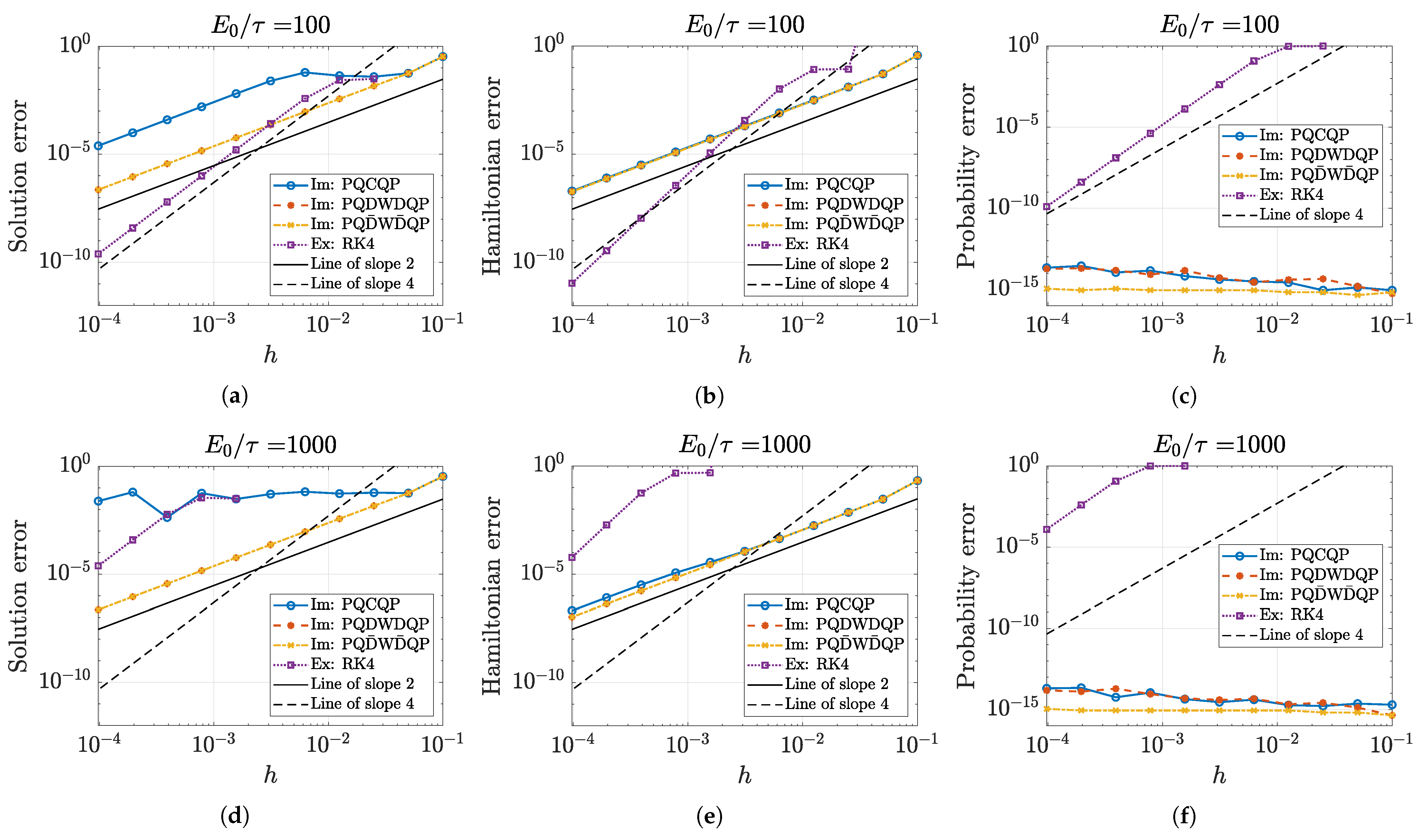
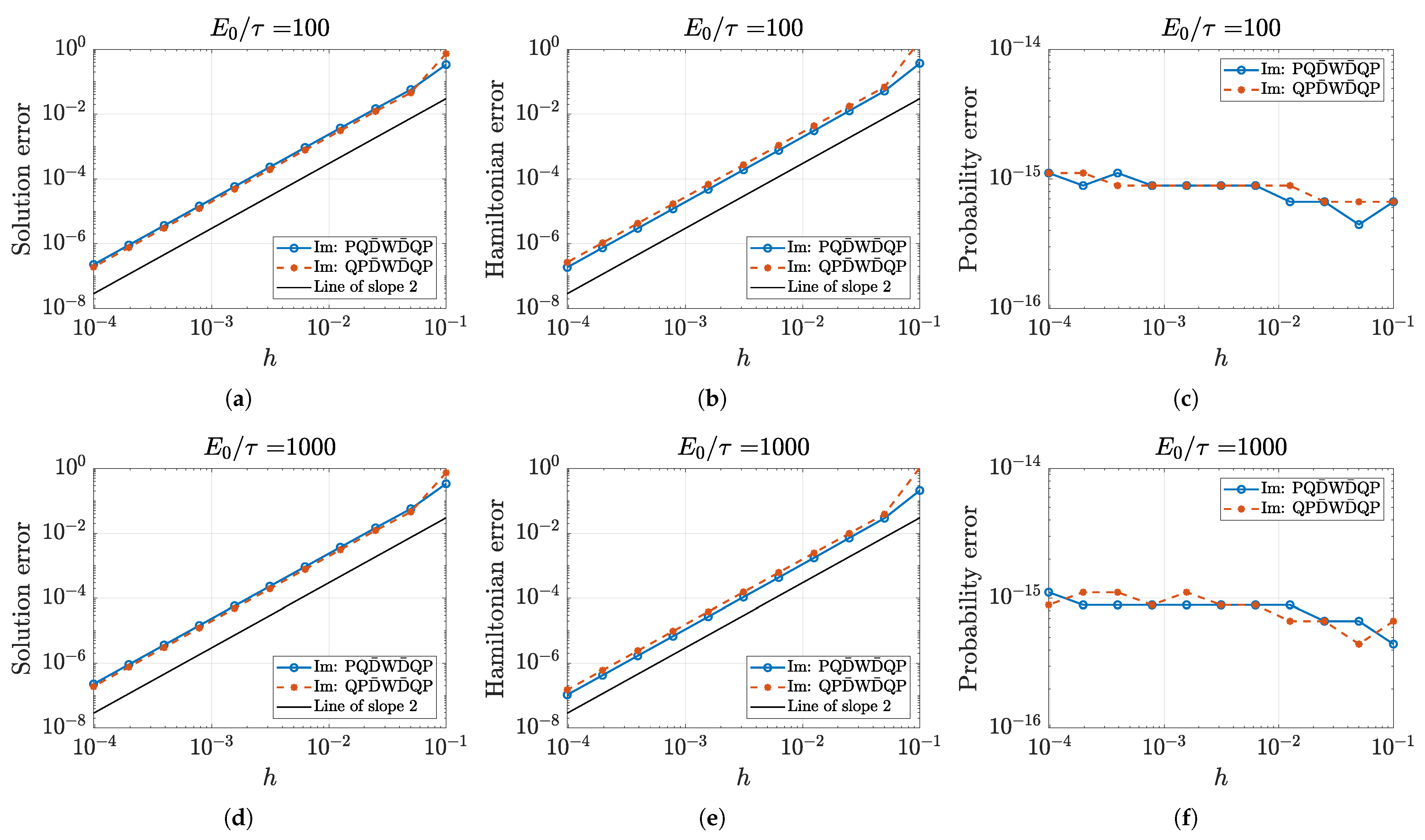
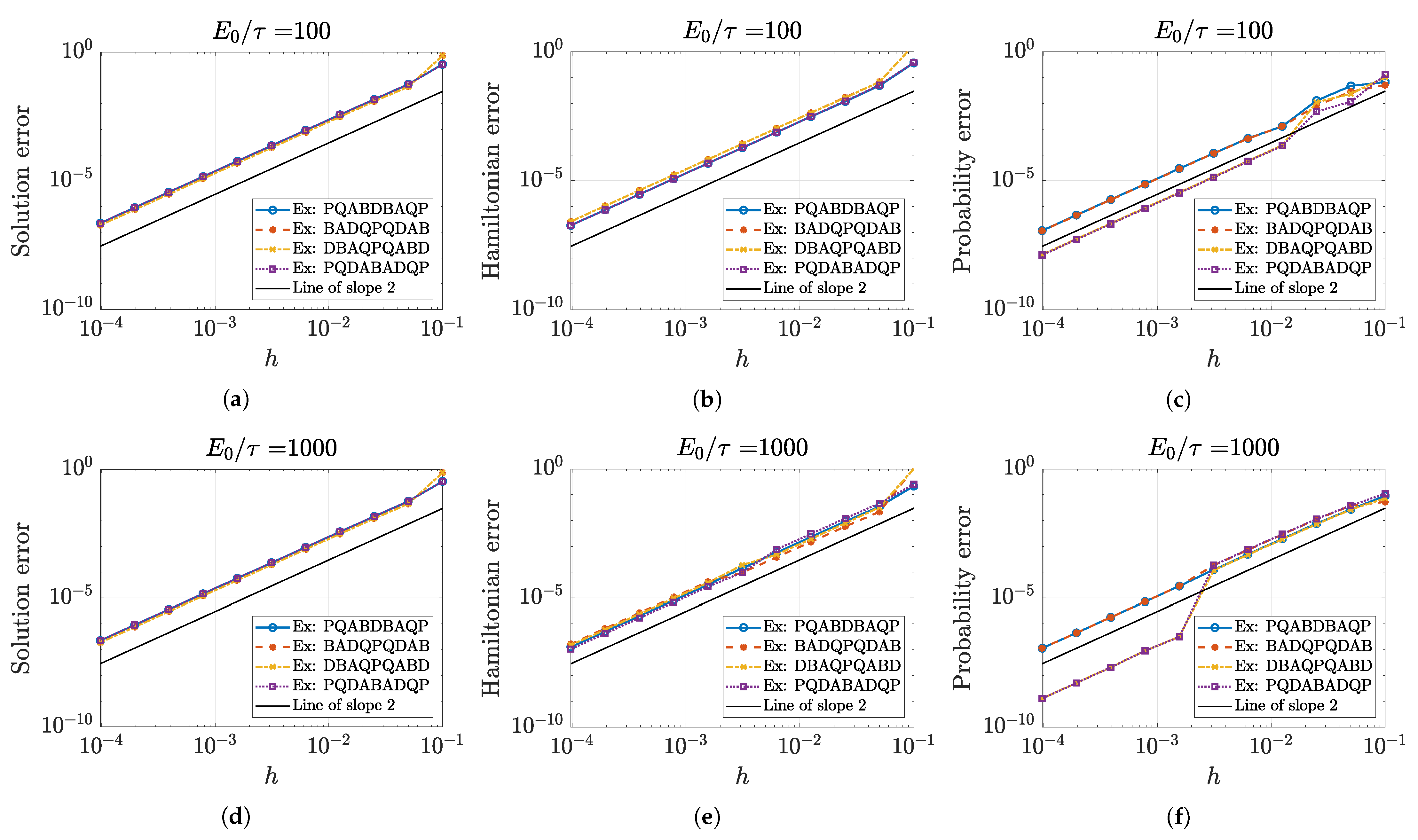
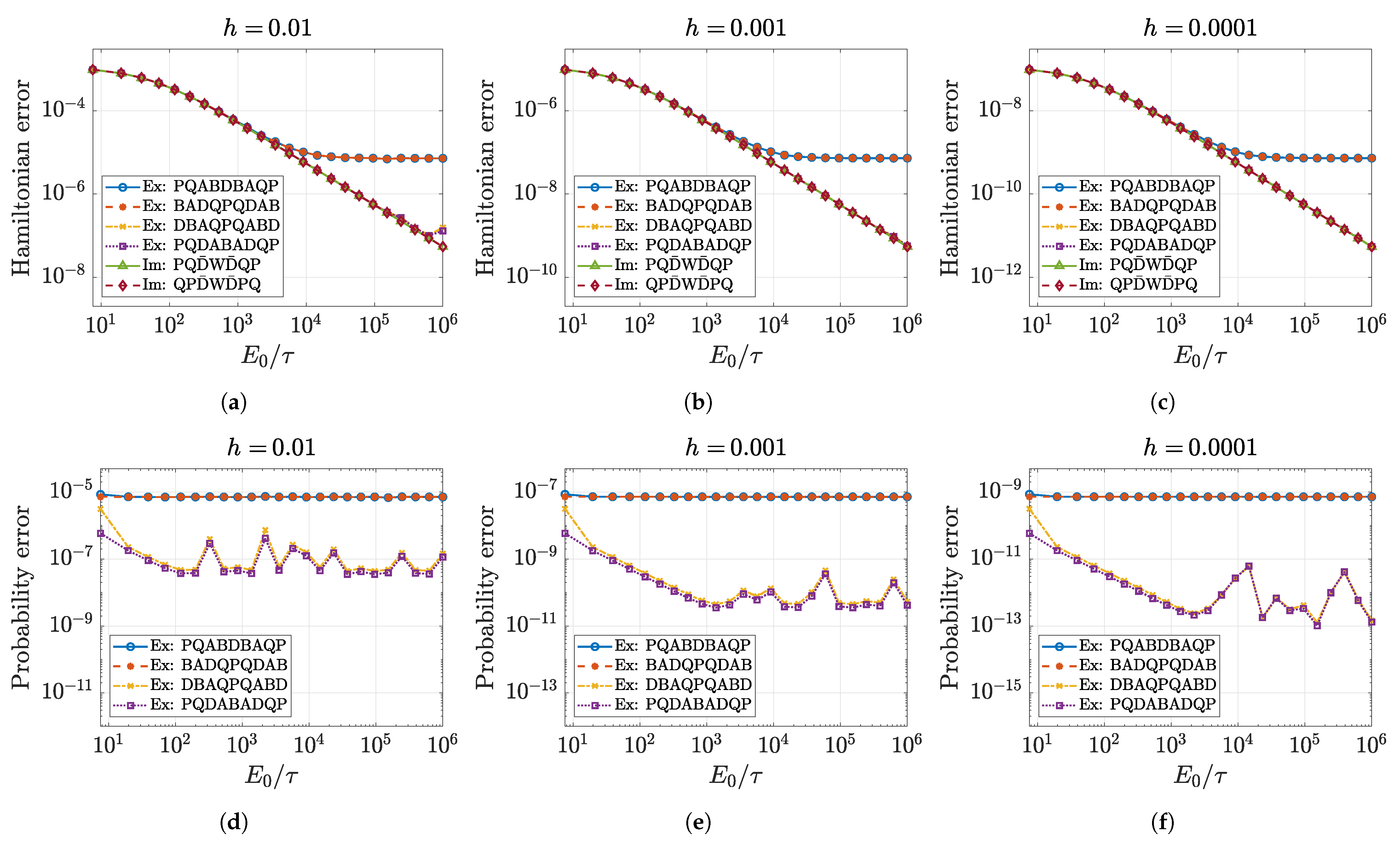
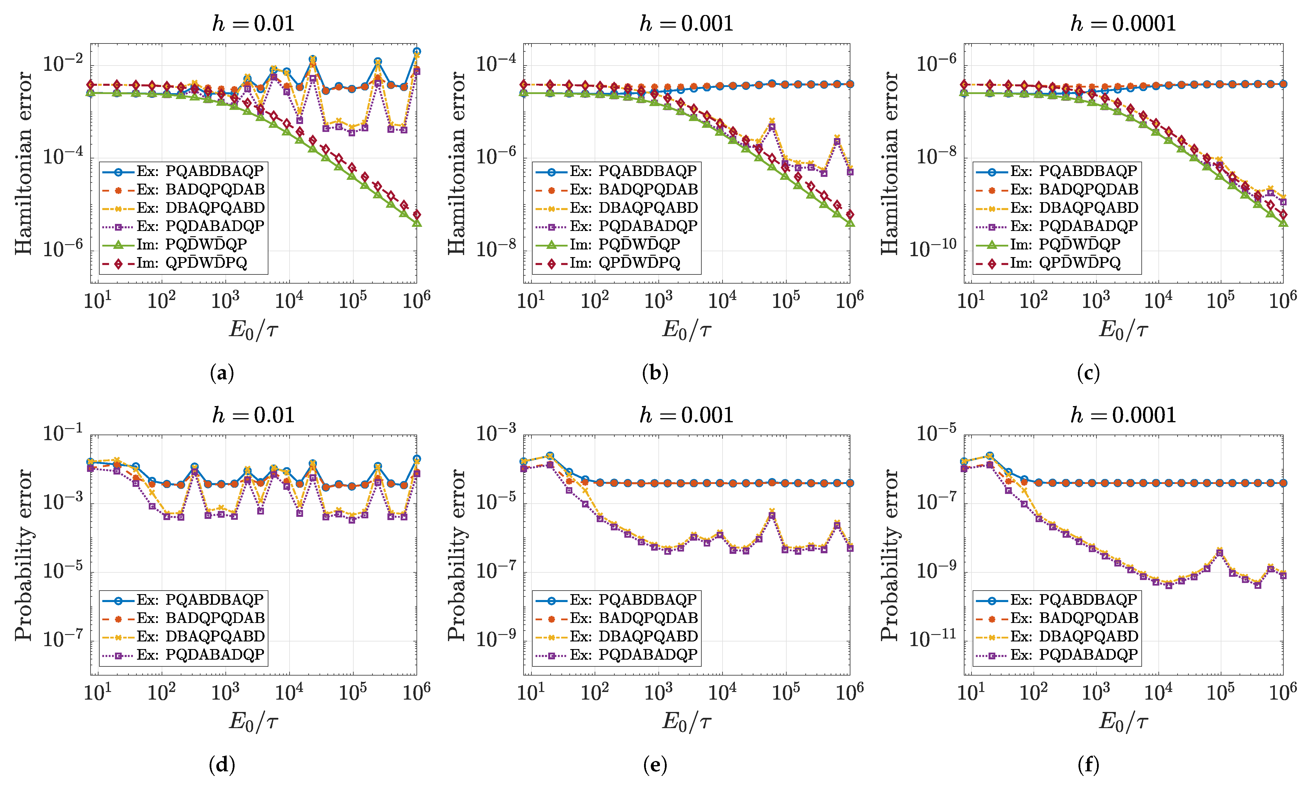
5.1. Approximation Order and Convergence

In this section, we numerically demonstrate the second-order approximation error and convergence of the proposed splitting methods of Section 4, and the importance of splitting the piece C into two pieces $\mathrm{D}$ and $\mathrm{W}$ for the semi-implicit splitting methods of Section 4.2 and splitting the piece $\mathrm{C}$ into three pieces, $\mathrm{D}$, $\mathrm{A}$, and $\mathrm{B}$, for the explicit splitting methods of Section 4.3. We integrate the model example (58)–(61) in time until $T_{end}=1$. For the reference “exact” solution, we consider the numerically computed solution of the explicit method $\mathrm{P}\mathrm{Q}\mathrm{D}\mathrm{A}\mathrm{B}\mathrm{A}\mathrm{D}\mathrm{Q}\mathrm{P}$ with the time step $h={10}^{-7}$. In Figure 2, Figure 3 and Figure 4 we illustrate numerical errors of the solution, the Hamiltonian (42), and the total charge probability (16) for different time step h values, i.e., left, middle, and right columns of the figures, respectively. To measure errors, we compute the maximal absolute error of the numerical solution at the final time $T_{end}$, while for the Hamiltonian and total charge probability, we consider maximal relative error over the whole computational time segment $[0,T_{end}]$. We demonstrate results for two different ratio $E_0/\tau$ values, i.e., when $E_0/\tau =100$ (top row) and $E_0/\tau =1000$ (bottom row).

In Figure 2, we plot errors of three semi-implicit splitting methods $\mathrm{P}\mathrm{Q}\mathrm{C}\mathrm{Q}\mathrm{P}$, $\mathrm{P}\mathrm{Q}\mathrm{D}\mathrm{W}\mathrm{D}\mathrm{Q}\mathrm{P}$ and $\mathrm{P}\mathrm{Q}\overline{\mathrm{D}}\mathrm{W}\overline{\mathrm{D}}\mathrm{Q}\mathrm{P}$ of Section 4.2. Not shown but equivalent results were obtained with the method $\mathrm{Q}\mathrm{P}\mathrm{C}\mathrm{P}\mathrm{Q}$ in place of $\mathrm{P}\mathrm{Q}\mathrm{C}\mathrm{Q}\mathrm{P}$ and with $Q=-1$. In addition to the proposed splitting methods, we have also added simulation results with the standard fourth-order Runge-Kutta method RK4, which requires four force evaluations per time step and it is neither symmetric nor symplectic. Figure 2a,d illustrate the second-order convergence of the splitting methods, while, as expected, RK4 is of order four. In order to better observe that, we have supplemented the figures with lines of slopes two and four, represented by the solid and dashed black lines, respectively.

Figure 2a,d demonstrate that the solution errors of both methods $\mathrm{P}\mathrm{Q}\mathrm{D}\mathrm{W}\mathrm{D}\mathrm{Q}\mathrm{P}$ and $\mathrm{P}\mathrm{Q}\overline{\mathrm{D}}\mathrm{W}\overline{\mathrm{D}}\mathrm{Q}\mathrm{P}$, which differ only by the rescaling (93), are indistinguishable. See also Figure 2b,e. They have much smaller solution errors compared to the method $\mathrm{P}\mathrm{Q}\mathrm{C}\mathrm{Q}\mathrm{P}$, where we have not split the piece C, and to RK4, especially for larger time steps h and ratio value $E_0/\tau$. Recall that the value $E_0/\tau$ appears in the charge dispersion relation (74) and produces high-frequency oscillations of the charge. From Figure 2, it is easy to see that to obtain stable numerical solutions with RK4 for large values of $E_0/\tau$, we require smaller time steps compared to the methods $\mathrm{P}\mathrm{Q}\mathrm{C}\mathrm{Q}\mathrm{P}$, $\mathrm{P}\mathrm{Q}\mathrm{D}\mathrm{W}\mathrm{D}\mathrm{Q}\mathrm{P}$, and $\mathrm{P}\mathrm{Q}\overline{\mathrm{D}}\mathrm{W}\overline{\mathrm{D}}\mathrm{Q}\mathrm{P}$. When $E_0/\tau \to 0$ (not shown), both methods $\mathrm{P}\mathrm{Q}\mathrm{C}\mathrm{Q}\mathrm{P}$ and $\mathrm{P}\mathrm{Q}\mathrm{D}\mathrm{W}\mathrm{D}\mathrm{Q}\mathrm{P}$ coincide and RK4 has smaller errors compared to the splitting methods, which can be attributed to fourth-order accuracy. Then, only in long-time simulations, the performance of splitting methods can be appreciated over RK4, since RK4 is a dissipative method. In addition, the case $E_0/\tau \to 0$ may not be of particular interest in modeling charge transfer in realistic crystals.

In Figure 2b,e, we demonstrate the maximal relative Hamiltonian errors and observe that with RK4, the Hamiltonian error converges at most with order four, and despite not splitting the piece $\mathrm{C}$ into two pieces $\mathrm{D}$ and $\mathrm{W}$, the $\mathrm{P}\mathrm{Q}\mathrm{C}\mathrm{Q}\mathrm{P}$ method’s Hamiltonian errors are almost indistinguishable from the Hamiltonian errors of the two methods $\mathrm{P}\mathrm{Q}\mathrm{D}\mathrm{W}\mathrm{D}\mathrm{Q}\mathrm{P}$ and $\mathrm{P}\mathrm{Q}\overline{\mathrm{D}}\mathrm{W}\overline{\mathrm{D}}\mathrm{Q}\mathrm{P}$. Figure 2c,f show, as expected, that RK4 does not exactly conserve the total charge probability (16) compared to all semi-implicit splitting methods. Notice that the method $\mathrm{P}\mathrm{Q}\overline{\mathrm{D}}\mathrm{W}\overline{\mathrm{D}}\mathrm{Q}\mathrm{P}$ conserves the total probability to machine precision due to the rescaling (93), while the errors for the other two methods $\mathrm{P}\mathrm{Q}\mathrm{C}\mathrm{Q}\mathrm{P}$ and $\mathrm{P}\mathrm{Q}\mathrm{D}\mathrm{W}\mathrm{D}\mathrm{Q}\mathrm{P}$ fluctuate close to double machine precision and slightly increase with smaller time steps. It is important to mention that in numerical results we did not observe differences between methods $\mathrm{P}\mathrm{Q}\mathrm{D}\mathrm{W}\mathrm{D}\mathrm{Q}\mathrm{P}$ and $\mathrm{P}\mathrm{Q}\overline{\mathrm{D}}\mathrm{W}\overline{\mathrm{D}}\mathrm{Q}\mathrm{P}$ and between methods $\mathrm{Q}\mathrm{P}\mathrm{D}\mathrm{W}\mathrm{D}\mathrm{P}\mathrm{Q}$ and $\mathrm{Q}\mathrm{P}\overline{\mathrm{D}}\mathrm{W}\overline{\mathrm{D}}\mathrm{P}\mathrm{Q}$. Thus, we postulate that the scaling of the charge variable c in (93) does not affect the numerical solution, at least in short-time simulations. In addition, the charge probability is conserved up to machine double-precision, as can be seen in Figure 2c,f, and does not increase with an increase in $T_{end}$.

The results of Figure 2 illustrate the importance of splitting the piece $\mathrm{C}$ such that numerical simulations can be performed with larger time steps. Thus, we will disregard the methods RK4, $\mathrm{P}\mathrm{Q}\mathrm{C}\mathrm{Q}\mathrm{P}$ and $\mathrm{Q}\mathrm{P}\mathrm{C}\mathrm{P}\mathrm{Q}$, from further numerical study and will concentrate on the methods $\mathrm{P}\mathrm{Q}\overline{\mathrm{D}}\mathrm{W}\overline{\mathrm{D}}\mathrm{Q}\mathrm{P}$ and $\mathrm{Q}\mathrm{P}\overline{\mathrm{D}}\mathrm{W}\overline{\mathrm{D}}\mathrm{P}\mathrm{Q}$ in place of the methods $\mathrm{P}\mathrm{Q}\mathrm{D}\mathrm{W}\mathrm{D}\mathrm{Q}\mathrm{P}$ and $\mathrm{Q}\mathrm{P}\mathrm{D}\mathrm{W}\mathrm{D}\mathrm{P}\mathrm{Q}$, respectively.

In Figure 3, we investigate the differences between the velocity and position semi-implicit splitting methods $\mathrm{P}\mathrm{Q}\overline{\mathrm{D}}\mathrm{W}\overline{\mathrm{D}}\mathrm{Q}\mathrm{P}$ and $\mathrm{Q}\mathrm{P}\overline{\mathrm{D}}\mathrm{W}\overline{\mathrm{D}}\mathrm{P}\mathrm{Q}$, respectively, for two different ratio $E_0/\tau$ values. As in Figure 2 and Figure 3, we plot the solution, Hamiltonian, and total probability errors for different time step h values. Figure 3a,d illustrate that the solution errors are very comparable with slightly smaller errors for the position method $\mathrm{Q}\mathrm{P}\overline{\mathrm{D}}\mathrm{W}\overline{\mathrm{D}}\mathrm{P}\mathrm{Q}$. On the contrary, the velocity splitting method $\mathrm{P}\mathrm{Q}\overline{\mathrm{D}}\mathrm{W}\overline{\mathrm{D}}\mathrm{Q}\mathrm{P}$, see Figure 3b,e, gives smaller Hamiltonian conservation errors of greater magnitude compared to the differences in the solution errors. Figure 3c,f show that both methods exactly conserve the total charge probability (16). Thus, we advocate the method $\mathrm{P}\mathrm{Q}\overline{\mathrm{D}}\mathrm{W}\overline{\mathrm{D}}\mathrm{Q}\mathrm{P}$ over the position splitting method $\mathrm{Q}\mathrm{P}\overline{\mathrm{D}}\mathrm{W}\overline{\mathrm{D}}\mathrm{P}\mathrm{Q}$ if Hamiltonian conservation is of higher importance. Recall that both methods are of the same computational complexity, see the discussion in Section 4.2 and Appendix A.2.

So far, in Figure 2 and Figure 3, we have investigated semi-implicit splitting methods that conserve exactly the charge probability, as presented in Section 4.2. In Figure 4, we demonstrate the approximation and the convergence order of the explicit splitting methods proposed in Section 4.3, i.e., we compare methods $\mathrm{P}\mathrm{Q}\mathrm{A}\mathrm{B}\mathrm{D}\mathrm{B}\mathrm{A}\mathrm{Q}\mathrm{P}$, $\mathrm{B}\mathrm{A}\mathrm{D}\mathrm{Q}\mathrm{P}\mathrm{Q}\mathrm{D}\mathrm{A}\mathrm{B}$, $\mathrm{D}\mathrm{B}\mathrm{A}\mathrm{Q}\mathrm{P}\mathrm{Q}\mathrm{A}\mathrm{B}\mathrm{D}$, and $\mathrm{P}\mathrm{Q}\mathrm{D}\mathrm{A}\mathrm{B}\mathrm{A}\mathrm{D}\mathrm{Q}\mathrm{P}$ for the same two ratio $E_0/\tau$ values. Figure 4 demonstrates that all explicit methods are second order. We do not observe significant differences between all four methods when the solution and Hamiltonian conservation errors are compared, see Figure 4a,b,d,e. Interesting differences appear in the total probability conservation, see Figure 4e,f. Figure 4e,f show a sudden drop in the total probability error at some time step h for the splitting methods $\mathrm{D}\mathrm{B}\mathrm{A}\mathrm{Q}\mathrm{P}\mathrm{Q}\mathrm{A}\mathrm{B}\mathrm{D}$ and $\mathrm{P}\mathrm{Q}\mathrm{D}\mathrm{A}\mathrm{B}\mathrm{A}\mathrm{D}\mathrm{Q}\mathrm{P}$ compared to the splitting methods $\mathrm{P}\mathrm{Q}\mathrm{A}\mathrm{B}\mathrm{D}\mathrm{B}\mathrm{A}\mathrm{Q}\mathrm{P}$ and $\mathrm{B}\mathrm{A}\mathrm{D}\mathrm{Q}\mathrm{P}\mathrm{Q}\mathrm{D}\mathrm{A}\mathrm{B}$. At which time step such drop in error occurs depends on the ratio $E_0/\tau$ value. In our numerical results (see also Figure 5 and Figure 6 from the following section), the drop in errors occurs when the absolute stability condition (91) in the form:

$$\left|h\frac{E_0}{\tau }\right|\le 2,$$

(102)

is satisfied. In future work, we plan to explore this from the analytic point of view. This observation also motivates to explore in future work multiple time-stepping approaches, where the charge part, e.g., $\mathrm{D}\mathrm{A}\mathrm{B}\mathrm{A}\mathrm{D}$ or $\mathrm{A}\mathrm{B}\mathrm{A}$ in method $\mathrm{P}\mathrm{Q}\mathrm{D}\mathrm{A}\mathrm{B}\mathrm{A}\mathrm{D}\mathrm{Q}\mathrm{P}$, is applied multiple times with smaller time step.

To even better indicate the differences between semi-implicit and all explicit splitting methods, we investigate in more detail the Hamiltonian and the total probability conservation errors for different ratio $E_0/\tau$ values in the following section.

5.2. Numerical Accuracy of Conserved Quantities

In the previous section, we numerically demonstrated the approximation and convergence orders of the proposed symplecticity-preserving symmetric splitting methods of Section 4 and showed the importance of splitting the piece $\mathrm{C}$, which allows us to obtain more accurate and stable results with larger time steps. In this section, we continue with a comparison of the semi-implicit and explicit splitting methods by investigating the conservation of several quantities for different values of $E_0/\tau$. In Figure 5 and Figure 6, we illustrate results for three different time step values, i.e., for $h=0.01$, $h=0.001$, and $h=0.0001$. The top row of Figure 5 and Figure 6 show the maximal relative error of the Hamiltonian (42), while the bottom row shows the maximal relative error of the total probability (16), over the computational time segment $[0,T_{end}]$, where $T_{end}=100$. Numerical simulations are performed for twenty-five different ratio $E_0/\tau$ values given by the following formula:

$$E_0^j/\tau =1000\frac{1.6^{j-1}-1}{1.6^{24}-1}{\tau }^{-1},j=1,\cdots ,25,$$

and errors are averaged over eleven numerical simulations with different initial conditions, which are described below.

In Figure 5 and Figure 6, we illustrate the results for two regimes of solutions, i.e., (approximately) linear and nonlinear, respectively. In the linear regime simulations, we generate eleven different initial conditions with $u_n$, $a_n$, $p_n$, and $b_n$ values for all n drawn from the uniform distribution $\mathcal{U}(-0.01,0.01)$. After the generation of values $a_n$ and $b_n$, we rescale them accordingly such that (16) holds. With these initial conditions, the charge probability is spread across the whole computational domain, and the lattice solutions are dominated by linear nonlocalized phonon waves. In the nonlinear regime, we generate eleven different initial initial conditions using patterns (100) and (101), where

$${\gamma }_j=0.4+j{h}_{\gamma },h_{\gamma }=0.05,j=0,\cdots ,10,$$

i.e., with $\gamma \in [0.4,0.9]$. With these initial conditions, we can generate nonlinear and localized solutions of charge transfer by mobile discrete breathers, e.g., see Figure 1. In addition, in both Figure 5 and Figure 6 with the reduction in the time step by a factor of 10, we have also reduced the y-axis scale by a factor of 100 to illustrate the second-order approximation error. We have also removed the probability errors for the semi-implicit splitting methods $\mathrm{P}\mathrm{Q}\overline{\mathrm{D}}\mathrm{W}\overline{\mathrm{D}}\mathrm{Q}\mathrm{P}$ and $\mathrm{Q}\mathrm{P}\overline{\mathrm{D}}\mathrm{W}\overline{\mathrm{D}}\mathrm{P}\mathrm{Q}$ from the probability error plots (bottom rows), since the total probability is conserved up to the machine precision, see Figure 3c,f.

In Figure 5a–c, it can clearly be seen that the Hamiltonian is conserved up to the second-order and that the errors of the semi-implicit methods $\mathrm{P}\mathrm{Q}\overline{\mathrm{D}}\mathrm{W}\overline{\mathrm{D}}\mathrm{Q}\mathrm{P}$ and $\mathrm{Q}\mathrm{P}\overline{\mathrm{D}}\mathrm{W}\overline{\mathrm{D}}\mathrm{P}\mathrm{Q}$ coincide very well with the errors of the explicit splitting methods $\mathrm{D}\mathrm{B}\mathrm{A}\mathrm{Q}\mathrm{P}\mathrm{Q}\mathrm{A}\mathrm{B}\mathrm{D}$ and $\mathrm{P}\mathrm{Q}\mathrm{D}\mathrm{A}\mathrm{B}\mathrm{A}\mathrm{D}\mathrm{Q}\mathrm{P}$ for all considered ratio $E_0/\tau$ values. Interestingly, as the value of $E_0/\tau$ increases, we observe significant differences in the Hamiltonian errors between the explicit methods. Such a large discrepancy cannot be seen in Figure 4b,e, since the results there were demonstrated for $E_0/\tau <{10}^4$. In Figure 4c,f, we observed that explicit methods $\mathrm{D}\mathrm{B}\mathrm{A}\mathrm{Q}\mathrm{P}\mathrm{Q}\mathrm{A}\mathrm{B}\mathrm{D}$ and $\mathrm{P}\mathrm{Q}\mathrm{D}\mathrm{A}\mathrm{B}\mathrm{A}\mathrm{D}\mathrm{Q}\mathrm{P}$ can have much smaller probability conservation errors compared to the methods $\mathrm{P}\mathrm{Q}\mathrm{A}\mathrm{B}\mathrm{D}\mathrm{B}\mathrm{A}\mathrm{Q}\mathrm{P}$ and $\mathrm{B}\mathrm{A}\mathrm{D}\mathrm{Q}\mathrm{P}\mathrm{Q}\mathrm{D}\mathrm{A}\mathrm{B}$. This observation is more evident in Figure 5d–f, where, in fact, the $\mathrm{P}\mathrm{Q}\mathrm{A}\mathrm{B}\mathrm{D}\mathrm{B}\mathrm{A}\mathrm{Q}\mathrm{P}$ and $\mathrm{B}\mathrm{A}\mathrm{D}\mathrm{Q}\mathrm{P}\mathrm{Q}\mathrm{D}\mathrm{A}\mathrm{B}$ methods’ Hamiltonians and probability errors are indistinguishable. Notice that the probability errors of the methods $\mathrm{D}\mathrm{B}\mathrm{A}\mathrm{Q}\mathrm{P}\mathrm{Q}\mathrm{A}\mathrm{B}\mathrm{D}$ and $\mathrm{P}\mathrm{Q}\mathrm{D}\mathrm{A}\mathrm{B}\mathrm{A}\mathrm{D}\mathrm{Q}\mathrm{P}$ precisely obey the second-order reduction in error only for $E_0/\tau$ values satisfying the condition (102). Despite that, the $\mathrm{D}\mathrm{B}\mathrm{A}\mathrm{Q}\mathrm{P}\mathrm{Q}\mathrm{A}\mathrm{B}\mathrm{D}$ and $\mathrm{P}\mathrm{Q}\mathrm{D}\mathrm{A}\mathrm{B}\mathrm{A}\mathrm{D}\mathrm{Q}\mathrm{P}$ methods’ probability errors are significantly smaller compared to the errors of the methods $\mathrm{P}\mathrm{Q}\mathrm{A}\mathrm{B}\mathrm{D}\mathrm{B}\mathrm{A}\mathrm{Q}\mathrm{P}$ and $\mathrm{B}\mathrm{A}\mathrm{D}\mathrm{Q}\mathrm{P}\mathrm{Q}\mathrm{D}\mathrm{A}\mathrm{B}$. In addition, the $\mathrm{P}\mathrm{Q}\mathrm{D}\mathrm{A}\mathrm{B}\mathrm{A}\mathrm{D}\mathrm{Q}\mathrm{P}$ method’s produced errors are slightly smaller compared to errors of the method $\mathrm{D}\mathrm{B}\mathrm{A}\mathrm{Q}\mathrm{P}\mathrm{Q}\mathrm{A}\mathrm{B}\mathrm{D}$.

The linear regime results, Figure 5, do not directly reflect the nonlinear regime results, see Figure 6. First of all, in the nonlinear regime, we observe larger Hamiltonian and probability errors comparing y-axis scales in Figure 5 and Figure 6. In all plots of Figure 6, we can see that two explicit methods $\mathrm{D}\mathrm{B}\mathrm{A}\mathrm{Q}\mathrm{P}\mathrm{Q}\mathrm{A}\mathrm{B}\mathrm{D}$ and $\mathrm{P}\mathrm{Q}\mathrm{D}\mathrm{A}\mathrm{B}\mathrm{A}\mathrm{D}\mathrm{Q}\mathrm{P}$, overall, outperform other two explicit methods $\mathrm{P}\mathrm{Q}\mathrm{A}\mathrm{B}\mathrm{D}\mathrm{B}\mathrm{A}\mathrm{Q}\mathrm{P}$ and $\mathrm{B}\mathrm{A}\mathrm{D}\mathrm{Q}\mathrm{P}\mathrm{Q}\mathrm{D}\mathrm{A}\mathrm{B}$, especially for larger values of $E_0/\tau$ and smaller time steps, with method $\mathrm{P}\mathrm{Q}\mathrm{D}\mathrm{A}\mathrm{B}\mathrm{A}\mathrm{D}\mathrm{Q}\mathrm{P}$ having slightly smaller errors compared to the method $\mathrm{D}\mathrm{B}\mathrm{A}\mathrm{Q}\mathrm{P}\mathrm{Q}\mathrm{A}\mathrm{B}\mathrm{D}$. We can also observe slightly smaller errors for the semi-implicit velocity method $\mathrm{P}\mathrm{Q}\overline{\mathrm{D}}\mathrm{W}\overline{\mathrm{D}}\mathrm{Q}\mathrm{P}$ compared to the position method $\mathrm{Q}\mathrm{P}\overline{\mathrm{D}}\mathrm{W}\overline{\mathrm{D}}\mathrm{P}\mathrm{Q}$, see Figure 6a–c, which can also be seen in Figure 3b,e, but not in the linear regime results of Figure 5a–c.

To summarize, after performing the computational analysis of the proposed splitting methods’ convergence and the conserved quantities’ conservation properties, we advocate the velocity semi-implicit, exactly charge-conserving method $\mathrm{P}\mathrm{Q}\overline{\mathrm{D}}\mathrm{W}\overline{\mathrm{D}}\mathrm{Q}\mathrm{P}$ over the position method $\mathrm{Q}\mathrm{P}\overline{\mathrm{D}}\mathrm{W}\overline{\mathrm{D}}\mathrm{P}\mathrm{Q}$ due to the smaller errors in the Hamiltonian conservation. From all the explicit splitting methods, we advocate the method $\mathrm{P}\mathrm{Q}\mathrm{D}\mathrm{A}\mathrm{B}\mathrm{A}\mathrm{D}\mathrm{Q}\mathrm{P}$, which showed overall smaller errors and conserves the total probability to a high degree in long-time simulations of charge transfer by discrete breathers as demonstrated in the following section.

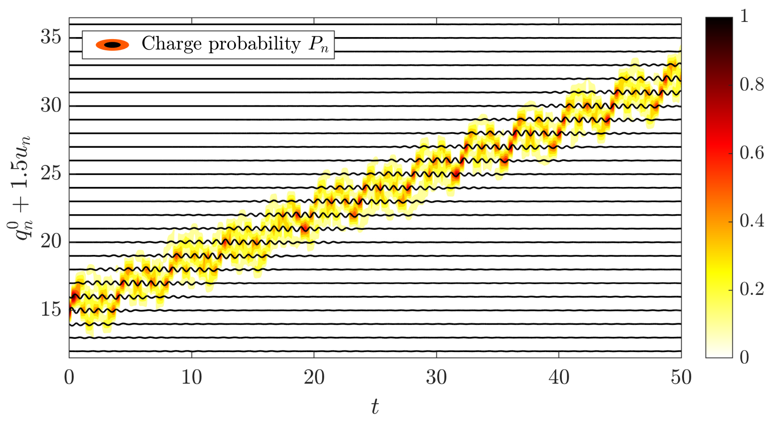
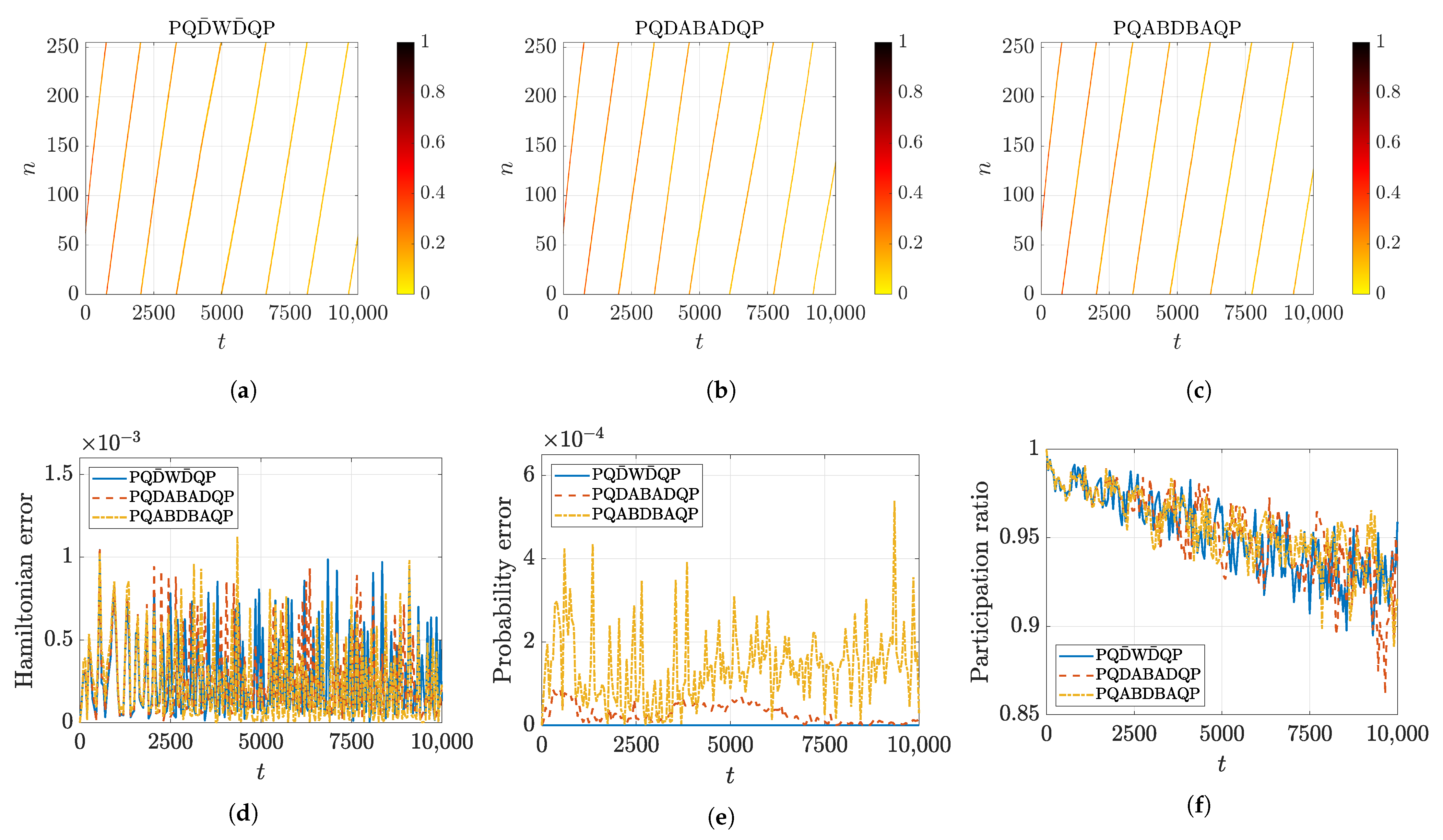
5.3. Charge Transfer by Mobile Discrete Breathers

In the example in Figure 1, we demonstrate charge transfer by a mobile discrete breather in time until $T_{end}=50$ initiated by the patterns (100) and (101) with $\gamma =0.6$ and computed with the explicit method $\mathrm{P}\mathrm{Q}\mathrm{D}\mathrm{A}\mathrm{B}\mathrm{A}\mathrm{D}\mathrm{Q}\mathrm{P}$ and time step $h=0.01$. In this section, we demonstrate the long-time charge transfer until $T_{end}={10}^4$ with the three proposed splitting methods of Section 4, i.e., with three lattice–charge–lattice methods $\mathrm{P}\mathrm{Q}\overline{\mathrm{D}}\mathrm{W}\overline{\mathrm{D}}\mathrm{Q}\mathrm{P}$, $\mathrm{P}\mathrm{Q}\mathrm{D}\mathrm{A}\mathrm{B}\mathrm{A}\mathrm{D}\mathrm{Q}\mathrm{P}$, and $\mathrm{P}\mathrm{Q}\mathrm{A}\mathrm{B}\mathrm{D}\mathrm{B}\mathrm{A}\mathrm{Q}\mathrm{P}$. Numerical simulations are performed in a lattice with $N=254$ particles, time step $h=0.01$, and $E_0/\tau =1000$. We excite the charge transfer with the patterns (100) and (101) set at $n^{*}=64$ with $\gamma =0.6$.

In Figure 7a–c, we plot contours of charge probability function $P_n\left(t\right)={\left|c_n\left(t\right)\right|}^2$ (15). All three methods illustrate localized charge transport by a mobile discrete breather, where short-time solutions appear indistinguishable. As time progresses, numerical solutions start to differ while producing qualitatively acceptable solutions. Importantly, such results are not possible to obtain with the methods RK4, $\mathrm{P}\mathrm{Q}\mathrm{C}\mathrm{Q}\mathrm{P}$ and $\mathrm{Q}\mathrm{P}\mathrm{C}\mathrm{P}\mathrm{Q}$ when $h=0.01$, see Figure 2d–f.

All three methods produce Hamiltonian (42) conservation errors to an equivalent degree over the whole computational time segment $[0,T_{end}]$, see Figure 7d. The same is not true for the total probability conservation (16), as can be seen in Figure 7e. Semi-implicit method $\mathrm{P}\mathrm{Q}\overline{\mathrm{D}}\mathrm{W}\overline{\mathrm{D}}\mathrm{Q}\mathrm{P}$ exactly conserves the total probability, while the explicit method $\mathrm{P}\mathrm{Q}\mathrm{D}\mathrm{A}\mathrm{B}\mathrm{A}\mathrm{D}\mathrm{Q}\mathrm{P}$ has smaller errors compared to the method $\mathrm{P}\mathrm{Q}\mathrm{A}\mathrm{B}\mathrm{D}\mathrm{B}\mathrm{A}\mathrm{Q}\mathrm{P}$, which is consistent with the results of Figure 6d.

To gain more information on the charge probability localization in charge transport by discrete breathers, in Figure 7f, we plot the normalized participation ratio (adopted from [19])

$${\mathrm{P}}_{\mathrm{r}}\left(t\right)=\frac{1}{N-1}\left(N\sum _{n=1}^N{P}_n{\left(t\right)}^2-1\right)/\sum _{n=1}^N{P}_n{\left(t\right)}^2\in [0,1],$$

as a function of time for all three methods. The participation ratio characterizes the localization of the charge probability, i.e., the larger the value of ${\mathrm{P}}_{\mathrm{r}}$, the more localized the charge probability is. For example, if the charge probability is completely localized at one site, then ${\mathrm{P}}_{\mathrm{r}}=1$, but in the situation when the charge probability is equally spread across the whole lattice, then ${\mathrm{P}}_{\mathrm{r}}=0$. With our charge probability’s initial excitation pattern (101), we have that ${\mathrm{P}}_{\mathrm{r}}\left(0\right)=1$. From Figure 7f, we can see that as the time progresses, the charge probability becomes more and more delocalized and eventually disperses within the lattice. We have verified this (not shown) by performing simulations with smaller time steps, and the phenomenon persists, which could be attributed to the properties of our example model of Section 2.7. Results of Figure 7f do not imply that charge transfer by mobile discrete breathers may not persist for longer times and distances in different lattice models. In addition, the excitation patterns (100)–(101) do not provide a means to produce exact time-periodic and space-translated traveling wave solutions of charge transfer by discrete breathers. It is still an open question if such solutions even exist. Overall, Figure 7 demonstrates that even the explicit, symplecticity-preserving, symmetric methods, which do not exactly preserve the charge probability (16), may produce qualitatively good long-time results with good approximate probability conservation properties compared to the exactly charge-probability conserving semi-implicit methods.

6. Discussion

In this work, we have constructed structure-preserving numerical methods for an important class of Hamiltonian equations to model charge transfer by intrinsic localized modes in nonlinear crystal lattice models. The importance of the study of charge transfer phenomena by lattice excitations cannot be overstated and traces back to original works by Landau L.D. and Pekar S.I. at the beginning of the last century. We demonstrate that such Hamiltonian equations can be written into a canonical form and address the question of solving the system of equations by direct numerical integration. The coupling of classically modeled lattice equations with the charge dynamics described by quantum mechanics presents serious challenges due to the different time scales of the charge and lattice dynamics, thus also inducing great important difficulties for the construction of stable, accurate, and efficient numerical integration schemes. In this work, we were able to address the problem by effective splitting strategies considering the structural properties of the equations splitting the piece $\mathrm{C}$ of charge dynamical equations into pieces $\mathrm{D}$ and $\mathrm{W}$ or into pieces $\mathrm{D}$, $\mathrm{A}$, and $\mathrm{B}$, as explained in Section 4.1.

In the construction of the splitting methods presented in Section 4, we have considered geometric structural properties of the Hamiltonian dynamics, i.e., symplecticity, which also implies phase volume preservation, time-reversibility, rotational invariance, and conserved quantities. We have derived two classes of computationally efficient splitting methods, i.e., semi-implicit and fully explicit methods. All the methods are symplectic, symmetric, second-order, and require a single calculation of the lattice force per time step and a single evaluation per time step of the lattice variable dependent terms in the charge equations. We have split the dynamical equations into pieces that correspond to explicit flow maps, which are Hamiltonian, symplectic, and time-reversible. The composition of flow maps will automatically inherit the same properties. However, to preserve the total charge probability, which is a quadratic invariant, and the rotational invariance of the probability amplitude, we require implicit methods for the pieces corresponding to the charge equations. One convenient method is, for example, the implicit midpoint rule. Since charge equations are linear with respect to the charge variables, we require only one solution of a linear system of equations per time step to exactly preserve the total charge probability and the rotational invariance of charge variables.

Performing numerical computational analysis for all the proposed splitting methods, we found that the Hamiltonian is conserved up to second-order in long-time simulations, which we would anticipate from symplectic integrators. The total charge probability is also preserved with high accuracy even with symplecticity-preserving symmetric explicit methods, which do not exactly conserve the total charge probability by design.

With both classes of methods, we were able to obtain qualitatively good numerical results of charge transfer by mobile discrete breathers, but it remains to be seen if the approximate charge probability conservation by explicit methods is sufficient to reproduce the physical properties of the phenomenon. Incoherencies may appear when post-processing the numerical results. To address this question we are developing multiple time-stepping methods based on the proposed symplectic explicit methods. In addition, explicit splitting methods do not preserve rotational invariance compared to the proposed semi-implicit methods. At this stage, it is unclear how important it is for the numerical method to preserve rotational invariance in connection to the study of charge transfer, but we conjecture that reproducing the physical properties of the equations is extremely beneficial. We will explore it in future work. It is also unclear at this stage if simulations with large time steps and second-order accuracy are sufficient to provide meaningful answers regarding charge transfer properties, despite the ability to obtain qualitatively good numerical results in long-time simulations. These considerations are of particular importance for spectral representation and theory, including simulations to find numerically exact periodic wave solutions with charge transfer and their stability, see [12,13].

When explicit splitting methods are compared, we find a peculiar sudden increase in accuracy in the total probability conservation at a certain time step, which is dependent on the charge oscillation frequency value $E_0/\tau$. We plan to address this phenomenon in a future work from an analytic point of view, in addition to multiple time-stepping or the development of the impulse method to improve probability conservation by explicit methods. Since all the proposed methods are only second-order, we plan to explore higher-order composition methods. It is well known that the number of equations to evaluate significantly increases with higher-order composition methods. An interesting prospect to potentially overcome this is to explore the so-called processing and effective order methods [37,38].

While the computational analysis was performed on an idealized example model, we have ensured sufficient generality by considering the charge energy function $E_n(q_1,\cdots ,q_N)$ to be dependent on the positions of the lattice particles. The developed methods can be directly applied to higher dimensional lattice models and with long-range interaction potentials. The flexibility of the methods stems from the fact that they can be directly incorporated into splitting methods of thermostated Hamiltonian dynamics and provide a means to construct other methods with multiple time-stepping and higher-order.

7. Conclusions

In this article, we have addressed the problem of numerical integration of conservative semi-classical systems, that is, a lattice of atoms, ions, or molecules that are described classically and a charge carrier that is described as a quantum particle within the tight-binding approximation. This approximation implies that the charge carrier states can be expressed in a basis of localized states at each atom or ion. The much faster dynamics of the charge carrier due to the small value of the mass of an electron and the very small value of the Planck constant provide serious challenges to numerical methods that attempt to resolve mathematical models of realistic systems. Importantly, numerical methods that do not conserve energy and the probability one of finding the charge carrier in the whole system can be viewed as unreliable.

We have solved the problem expressing the whole system in a canonical form and designing integration schemes based on the splitting methods approach. We have proposed different algorithms with the objective of conserving the underlying properties of the original mathematical model, i.e., symplecticity, time-reversibility, conservation of the total charge probability and the Hamiltonian, rotational invariance of the charge variables, and allowing computations with large time steps and small numerical errors. We have tested these methods producing polarobreathers, i.e., breathers transporting charge probability, in a phenomenological model for silicates. Polarobreathers are good candidates to explain experimental results on charge transport without an electric field.

We have demonstrated that explicit splitting methods conserve the Hamiltonian up to the second order and approximately conserve the charge probability in long-time simulations. However, semi-implicit methods conserve the charge probability and the rotational invariance of the charge-probability amplitude exactly. They also have smaller or on par numerical errors compared to the explicit methods. Moreover, the proposed semi-implicit methods allow larger time steps with smaller errors than other conventional methods. Therefore, at least for small models, they are the method of choice for integration of semi-classical systems. Further developments of the explicit methods are highly motivated by the numerical integration of charge transfer in two- and three-dimensional crystal lattice models, where solutions of a large linear system of equations for charge variables per time can become very cumbersome.

The methods are not limited to the systems tested as they rely on the generic properties of tight-binding semi-classical models, which are a consequence of the first principles and the laws of physics, particularly classical Hamiltonian dynamics and the Schrödinger equations. We think that the proposed methods will provide efficient computational means to study the phenomenon of charge transfer by nonlinear lattice excitations in physical and biological lattice models with realistic potentials and applications.

References

1. Landau, L.D. Electron motion in crystal lattices. Phys. Z. Sowjetunion 1933, 3, 664. [Google Scholar]
2. Pekar, S.I. Local quantum states of electrons in an ideal ion crystal. J. Phys. USSR 1946, 10, 341. (In German) [Google Scholar]
3. Landau, L.D.; Pekar, S.I. Effective mass of a polaron. Zh. Eksp. Teor. Fiz. 1948, 18, 419–423, English translation: Ukr. J. Phys., Special Issue: 2008, 53, 71–74. [Google Scholar]
4. Alexandrov, A.S. Polarons in Advanced Materials; Springer Series in Materials Science; Springer: Dordrecht, The Netherlands, 2007. [Google Scholar]
5. Ashcroft, N.W.; Mermim, N.D. Solid State Physics, 1st ed.; Cengage Learning: Boston, MA, USA, 1976. [Google Scholar]
6. Holstein, T. Studies of polaron motion: Part I. The molecular-crystal model. Ann. Phys. 1959, 8, 325–342. [Google Scholar] [CrossRef]
7. Holstein, T. Studies of polaron motion: Part II. The “small” polaron. Ann. Phys. 1959, 8, 343–389. [Google Scholar] [CrossRef]
8. Braun, O.M.; Kivshar, Y.S. Nonlinear dynamics of the Frenkel-Kontorova model. Phys. Rep. 1998, 1–2, 1–108. [Google Scholar] [CrossRef]
9. Braun, O.M.; Kivshar, Y.S. The Frenkel-Kontorova Model; Springer: Berlin, Germany, 2004. [Google Scholar]
10. Davydov, A.S. Solitons in Molecular Systems; Mathematics and Its Applications; Springer Dordrecht: Dordrecht, The Netherlands, 1985. [Google Scholar]
11. Sievers, A.J.; Takeno, S. Intrinsic Localized Modes in Anharmonic Crystals. Phys. Rev. Lett. 1988, 61, 970–973. [Google Scholar] [CrossRef]
12. Archilla, J.F.R.; Doi, Y.; Kimura, M. Pterobreathers in a model for a layered crystal with realistic potentials: Exact moving breathers in a moving frame. Phys. Rev. E 2019, 100, 022206. [Google Scholar] [CrossRef]
13. Bajārs, J.; Archilla, J.F.R. Frequency-momentum representation of moving breathers in a two dimensional hexagonal lattice. Physica D 2022, 441, 133497. [Google Scholar] [CrossRef]
14. Aubry, S. Breathers in nonlinear lattices: Existence, linear stability and quantization. Physica D 1997, 103, 201–250. [Google Scholar] [CrossRef]
15. Kalosakas, G.; Aubry, S. Polarobreathers in a generalized Holstein model. Physica D 1998, 113, 228–232. [Google Scholar] [CrossRef]
16. Cuevas, J.; Kevrekidis, P.G.; Frantzeskakis, D.J.; Bishop, A.R. Existence of bound states of a polaron with a breather in soft potentials. Phys. Rev. B 2006, 74, 064304. [Google Scholar] [CrossRef]
17. Hennig, D. Electron-vibron-breather interaction. Phys. Rev. E 2000, 62, 2846–2857. [Google Scholar] [CrossRef] [PubMed]
18. Velarde, M. From polaron to solectron: The addition of nonlinear elasticity to quantum mechanics and its possible effect upon electric transport. J. Comput. Appl. Math. 2010, 233, 1432–1445. [Google Scholar] [CrossRef]
19. Ros, O.G.C.; Cruzeiro, L.; Velarde, M.G.; Ebeling, W. On the possibility of electric transport mediated by long living intrinsic localized solectron modes. Eur. Phys. J. B 2011, 80, 545–554. [Google Scholar]
20. Cruzeiro-Hansson, L.; Eilbeck, J.C.; Marín, J.L.; Russell, F.M. Breathers in systems with intrinsic and extrinsic nonlinearities. Physica D 2000, 142, 101–112. [Google Scholar] [CrossRef]
21. Archilla, J.F.R.; Jiménez, N.; Sánchez-Morcillo, V.J.; García-Raffi, L.M. (Eds.) Quodons in Mica: Nonlinear Localized Travelling Excitations in Crystals; Springer Series in Materials Science; Springer: Cham, Switzerland, 2015; Volume 221. [Google Scholar]
22. De Moura, F. Numerical evidence of electron–soliton dynamics in Fermi–Pasta–Ulam disordered chains. Physica D 2013, 253, 66–72. [Google Scholar] [CrossRef]
23. Archilla, J.F.R.; Zolotaryuk, Y.; Kosevich, Y.A.; Doi, Y. Nonlinear waves in a model for silicate layers. Chaos 2018, 28, 083119. [Google Scholar] [CrossRef]
24. Archilla, J.F.R.; Russell, F.M. On the charge of quodons. Lett. Mater. 2016, 6, 3–8. [Google Scholar] [CrossRef]
25. Russell, F.M.; Archilla, J.F.R.; Frutos, F.; Medina-Carrasco, S. Infinite charge mobility in muscovite at 300 K. EPL 2017, 120, 46001. [Google Scholar] [CrossRef]
26. Russell, F.M.; Russell, A.W.; Archilla, J.F.R. Hyperconductivity in fluorphlogopite at 300 K and 1.1 T. EPL 2019, 127, 16001. [Google Scholar] [CrossRef]
27. Russell, F.M.; Archilla, J.F.R. Ballistic charge transport by mobile nonlinear excitations. Phys. Status Solidi RRL 2022, 16, 2100420. [Google Scholar] [CrossRef]
28. Russell, F.M.; Archilla, J.F.R.; Medina-Carrasco, S. Localized Waves in Silicates. What Do We Know from Experiments? In 13th Chaotic Modeling and Simulation International Conference; Skiadas, C., Dimotikalis, Y., Eds.; Springer: Berlin, Germany, 2021; pp. 721–734. [Google Scholar]
29. MacKay, R.S.; Aubry, S. Proof of existence of breathers for time-reversible or Hamiltonian networks of weakly coupled oscillators. Nonlinearity 1994, 7, 1623–1643. [Google Scholar] [CrossRef]
30. Aubry, S. Discrete Breathers: Localization and transfer of energy in discrete Hamiltonian nonlinear systems. Physica D 2006, 216, 1–30. [Google Scholar] [CrossRef]
31. Flach, S.; Gorbach, A. Discrete breathers—Advances in theory and applications. Phys. Rep. 2008, 467, 1–116. [Google Scholar] [CrossRef]
32. Marín, J.L.; Russell, F.M.; Eilbeck, J.C. Breathers in cuprate-like lattices. Phys. Lett. A 2001, 281, 21–25. [Google Scholar] [CrossRef]
33. Dou, Q.; Cuevas, J.; Eilbeck, J.C.; Russell, F.M. Breathers and kinks in a simulated crystal experiment. Discrete Cont. Dyn. Ser. S 2011, 4, 1107–1118. [Google Scholar] [CrossRef]
34. Bajārs, J.; Eilbeck, J.C.; Leimkuhler, B. Nonlinear propagating localized modes in a 2D hexagonal crystal lattice. Physica D 2015, 301-302, 8–20. [Google Scholar] [CrossRef]
35. Bajārs, J.; Eilbeck, J.C.; Leimkuhler, B. Two-dimensional mobile breather scattering in a hexagonal crystal lattice. Phys. Rev. E 2021, 103, 022212. [Google Scholar] [CrossRef]
36. Leimkuhler, B.; Matthews, C. Molecular Dynamics: With Deterministic and Stochastic Numerical Methods; Springer: Berlin, Germany, 2015. [Google Scholar]
37. Hairer, E.; Lubich, C.; Wanner, G. Geometric Numerical Integration: Structure-Preserving Algorithms for Ordinary Differential Equations; Springer Science & Business Media: Berlin, Germany, 2006. [Google Scholar]
38. Blanes, S.; Casas, F.; Murua, A. Splitting and composition methods in the numerical integration of differential equations. Boletin de la Sociedad Espanola de Matematica Aplicada 2008, 45, 89–145. [Google Scholar]
39. Yoshida, H. Construction of higher order symplectic integrators. Phys. Lett. A 1990, 150, 262–268. [Google Scholar] [CrossRef]
40. Suzuki, M. General theory of higher-order decomposition of exponential operators and symplectic integrators. Phys. Lett. A 1992, 165, 387–395. [Google Scholar] [CrossRef]
41. Cohen-Tannoudji, C.; Diu, B.; Laloe, F. Quantum Mechanics, Vol. 1: Basic Concepts, Tools, and Applications, 2nd ed.; Wiley-VCH: Weinheim, Germany, 2019. [Google Scholar]
Figure 1. Charge transfer by a mobile discrete breather in the model example of Section 2.7. Solid lines indicate the lattice particle displacements amplified by the factor 1.5 , while the color plot illustrates the probability of finding the charge at a lattice site at a given time. Numerical results are obtained with the explicit, symplecticity-preserving, symmetric numerical method P Q D A B A D Q P , see Section 4.3. See also Section 5 for additional numerical results of charge transfer by discrete breathers.
Mathematics 10 03460 g001
Figure 2. Numerical convergence study of the semi-implicit splitting methods: P Q C Q P , P Q D W D Q P , and P Q D ¯ W D ¯ Q P , compared to the fourth-order explicit Runge-Kutta method RK4. Top (ac): E 0 / τ = 100 . Bottom (df): E 0 / τ = 1000 . Left (a,d): maximal absolute error of the solution at time t = 1 . Middle (b,e): maximal relative error of the Hamiltonian (42) for t [ 0 , 1 ] . Right (c,f): maximal relative error of the total charge probability (16) for t [ 0 , 1 ] . The numerical solution of reference is computed with the method P Q D A B A D Q P and time step h = 10 7 and with initial conditions given by the patterns (100) and (101), where γ = 0.6 .
Mathematics 10 03460 g002
Figure 3. Numerical convergence study of the semi-implicit splitting methods: P Q D W D Q P and Q P D ¯ W D ¯ P Q . Top (ac): E 0 / τ = 100 . Bottom (df): E 0 / τ = 1000 . Left (a,d): maximal absolute error of the solution at t = 1 . Middle (b,e): maximal relative error of the Hamiltonian (42) for t [ 0 , 1 ] . Right (c,f): maximal relative error of the total charge probability (16) for t [ 0 , 1 ] . The numerical solution of reference is computed with the method P Q D A B A D Q P and time step h = 10 7 and with initial conditions given by the patterns (100) and (101), where γ = 0.6 .
Mathematics 10 03460 g003
Figure 4. Numerical convergence study of the explicit splitting methods: P Q A B D B A Q P , B A D Q P Q D A B , D B A Q P Q A B D , and P Q D A B A D Q P . Top (ac): E 0 / τ = 100 . Bottom (df): E 0 / τ = 1000 . Left (a,d): maximal absolute error of the solution at t = 1 . Middle (b,e): maximal relative error of the Hamiltonian (42) for t [ 0 , 1 ] . Right (c,f): maximal relative error of the total charge probability (16) for t [ 0 , 1 ] . The numerical solution of reference is computed with the method P Q D A B A D Q P and time step h = 10 7 , and with initial conditions given by the patterns (100) and (101), where γ = 0.6 .
Mathematics 10 03460 g004
Figure 5. Hamiltonian and total probability conservation errors of the splitting methods: P Q A B D B A Q P , B A D Q P Q D A B , D B A Q P Q A B D , P Q D A B A D Q P , P Q D ¯ W D ¯ Q P , and Q P D ¯ W D ¯ P Q . Top (ac): maximal relative error of the Hamiltonian (42) for t [ 0 , 100 ] . Bottom (df): maximal relative error of the total charge probability (16) for t [ 0 , 100 ] , where the results for semi-implicit methods are excluded. Left (a,d): time step h = 0.01 . Middle (b,e): time step h = 0.001 . Right (c,f): time step h = 0.0001 . The Hamiltonian and probability errors are averaged over eleven numerical simulations with randomly generated initial conditions from the uniform distribution U ( 0.01 , 0.01 ) .
Mathematics 10 03460 g005
Figure 6. Hamiltonian and total probability conservation errors of the splitting methods: P Q A B D B A Q P , B A D Q P Q D A B , D B A Q P Q A B D , P Q D A B A D Q P , P Q D ¯ W D ¯ Q P , and Q P D ¯ W D ¯ P Q . Top (ac): maximal relative error of the Hamiltonian (42) for t [ 0 , 100 ] . Bottom (df): maximal relative error of the total charge probability (16) for t [ 0 , 100 ] , where results for semi-implicit methods are excluded. Left (a,d): time step h = 0.01 . Middle (b,e): time step h = 0.001 . Right (c,f): time step h = 0.0001 . The Hamiltonian and probability errors are averaged over eleven numerical simulations with initial conditions (100) and (101) and different values of γ [ 0.4 , 0.9 ] .
Mathematics 10 03460 g006
Figure 7. Simulation of charge transfer by a mobile discrete breather with three splitting methods: P Q D ¯ W D ¯ Q P , P Q D A B A D Q P , and P Q A B D B A Q P . The solutions are initiated with patterns (100) and (101), where γ = 0.6 . Other parameter values: h = 0.01 , N = 254 and T e n d = 10 4 . Top (ac): contours of the charge probability P n . Bottom: (d) relative error of the Hamiltonian (42) at each time step; (e) relative error of the total charge probability (16) at each time step; (f) participation ratio value at each time step.
Mathematics 10 03460 g007
Publisher’s Note: MDPI stays neutral with regard to jurisdictional claims in published maps and institutional affiliations.