Abstract
Bulk-service queueing systems have been widely applied in many areas in real life. While single-server queueing systems work in some cases, multi-servers can efficiently handle most complex applications. Bulk-service, multi-server queueing systems (compared to well-developed single-server queueing systems) are more complex and harder to deal with, especially when the inter-arrival time distributions are arbitrary. This paper deals with analytic and computational analyses of queue-length distributions for a complex bulk-service, multi-server queueing system GI/M/c, wherein inter-arrival times follow an arbitrary distribution, a is the quorum, and b is the capacity of each server; service times follow exponential distributions. The introduction of quorum a further increases the complexity of the model. In view of this, a two-dimensional Markov chain has to be involved. Currently, it appears that this system has not been addressed so far. An elegant analytic closed-form solution and an efficient algorithm to obtain the queue-length distributions at three different epochs, i.e., pre-arrival epoch (p.a.e.), random epoch (r.e.), and post-departure epoch (p.d.e.) are presented, when the servers are in busy and idle states, respectively.
MSC:
60-08; 60J27
1. Introduction
Queueing theory consists of a powerful tool for modelling and analytically studying many complex systems, such as computer networks, banks, telecommunications, manufacturing, and transportation systems. Compared to well-developed single-server non-bulk queueing systems, bulk-service systems have an extensive mathematical theory. They are more complex and harder to deal with. In a bulk-service queue, a group (or batch) of customers can be served simultaneously. Examples of their applications can be seen in shuttle-bus services, freight trains, express elevators, tour operators, and batch servicing in manufacturing processes. This topic, due to its perceived applicability, has attracted the attention of many researchers over several decades. At an early stage, some simple bulk-service models, such as single-server systems GI/Mb/1 and M/Ma/1 were studied by Shyu [1] and Gross et al. [2], respectively. Neuts [3] first introduced a quorum bulk service rule to create more complex models necessary to describe certain realistic situations. He considered a queueing system with Poisson arrivals and a general service-time distribution M/G/1, where a is the quorum and b is the capacity of the server. Easton and Chaudhry [4] extended these results to the case where the inter-arrival times were Erlangian with the -stage, E/M/1. Later, Chaudhry and Madill [5] gave a solution for a more general queueing system GI/M/1. An alternate method was given in Neuts’ book [6], wherein he describes the application of his matrix geometric approach to the GI/PH/1 system, which has a phase-type service-time distribution. However, these systems are single-server queues. For many other variations of bulk-service queues, such as bulk service queues with vacations or bulk-service queues of the type M/G/1, one may view the survey paper written by Sasikala and Indhira [7]. In this survey, which had over 100 publications, most of the models considered were single server queues.
Multi-server queueing systems are an important class of queueing processes and have broad practical applications. However, such systems are more complex and harder to deal with compared to single-server queueing systems, especially when the inter-arrival time distribution is arbitrary. Medhi [8] investigated a queue with Poisson arrivals M/G/c, but his method was not analytically tractable for . Related work has also been conducted by Sim [9] on M/M/c by using algorithmic methods but no numerical results were given. Sim [10] solved the -phase Erlangian arrivals E/M/c system for the random epoch probabilities in the steady state and discussed his results in the context of a transportation system. Adan and Resing [11] derived and presented the numerical results of the queue-length distributions for models M/COXIAN-2/c and M/E/c. Compared to our model GI/M/c, the most relevant model studied by other researchers was GI/Mb/c, where the quorum was set to 1. Goswami et al. [12] solved the finite-buffer GI/Mb/c model by the supplementary variable technique. Shyu [13], as well as Chaudhry and Templeton [14], dealt with the distribution of the number of customers in the system without considering the server being busy or idle. Therefore, there is no information regarding server utilization. Moreover, the numerical results for the system GI/Mb/c are not available.
To make the model useful for applications, in this paper, we considered analytic and computational aspects to determine the performance of a complex bulk-service, multi-server queueing system GI/M/c. The model GI/M/c is an extension of the system GI/Mb/c (Shyu [13] as well as by Chaudhry and Templeton [14]), by introducing quorum in the multi-server system GI/Mb/c. A quorum refers to the minimum number of customers that are required in the waiting line before service commences, e.g., a ferry will not start until the quorum is met, or if we are dealing with transportation problems, a bus may not start until we have the quorum. This is an important policy desired by the service providers to reduce the business cost and maximize server utilization. The adding of the quorum policy makes the model closer to the real situation, but it also makes the model more complex to study. In view of this, a two-dimensional Markov chain has to be involved where the first dimension corresponds to the state of the servers (busy or idle) and the second dimension corresponds to the number of customers in the queue. We give an elegant analytic closed-form solution to obtain the queue-length distributions at three different epochs, such as pre-arrival epoch (p.a.e.), random epoch (r.e.), and post-departure epoch (p.d.e.), not only for the system in a busy state, but also in an idle state. In the case of the idle state, the probabilities were obtained by simultaneously solving the equations, some of which contained infinite series, which needed to be truncated to obtain the results. Instead of truncation, which leads to approximate results, we derived a closed-form solution and proposed an efficient algorithm to fix this problem. The model GI/M/c that we considered includes most models ([1,2,4,5,6,8,9,10,13,14]) as special cases. Our model was validated in giving numerical results with the desired degree of accuracy and trivial computational costs. By selecting particular numbers for the parameters and c, and inter-arrival time distributions, the numerical results produced by our model match the ones provided in those simpler models as expected.
The paper is organized as follows. In the following section, we describe the queueing model GI/M/c, and establish a transition probability matrix (t.p.m.) for the system in Section 3. In Section 4, Section 5 and Section 6, we obtain the queue-length distributions at three different epochs, such as pre-arrival epoch (p.a.e.), random epoch (r.e.), and post-departure epoch (p.d.e.). To make the model useful for applications, sample numerical results are provided in Section 7.
2. Model Description
In this continuous-time queueing system GI/M/c, there are c independent servers, each serving at the rate . The customers arrive at the rate according to a renewal process with an arbitrary inter-arrival time distribution . One of the idle c servers starts the service as soon as the number of customers (including the new arriving customer) in the queue reaches quorum a. Each c server is able to serve up to b customers simultaneously. This indicates that if the server completes a service and finds less than the quorum a in the queue, it will become idle until a is reached. The service times of each server are independently–identically exponentially distributed random variables (i.i.e.d.r.v.s). We consider the system to be in a steady state with the traffic intensity . The queue discipline is first-come first-serve (FCFS) by batches.
3. Transition Probability Matrix (t.p.m.)
In the queueing system GI/M/c, the states occurring at the instants immediately before the arrivals form an embedded Markov chain (I.M.C.). The state seen by an arriving customer can be described by , where is the queue-length and is a supplementary flag defined as
We define the system as busy if all the servers are busy (), and idle if at least one server is idle ( is the number of idle servers). The queue-length n can be written as , where q is the nearest lower non-negative integer of the fraction n/b, denoting the available number of full size batches (the batch size is b) in the queue waiting for service.
To build a t.p.m. of the system, we first define the following probabilities.
- and , where , and there are less than a customers waiting in the queue at the beginning of the period, thus . Here,is the conditional probability that l of m servers complete services during an inter-arrival period of duration t, given that m servers are busy ( servers are idle) at the beginning of the period. Moreover, is defined as
- is the conditional probability that l of c servers become idle during an inter-arrival period, given that all c servers are busy at the beginning of the period, and q batches of customers are waiting for the services. Assume that a time V has elapsed when the last batch of q batches enters service. In this case, the c servers have been processed at a rate of until time V has elapsed. When all c servers are busy, the number of departed batches follows a Poisson process with a rate . The time V is Erlang-distributed, so it is the sum of q exponential random variables with a rate , implying that the probability density function (p.d.f.) of V is given byAfter all the waiting q batches leave the queue, there is time remaining to have l batches processed. The probability that these l batches complete the service during period is . Therefore
- is the conditional probability that l batches complete service during an inter-arrival period of duration t, given that all the c servers are busy at the beginning of the period and still busy at the end of the period. In this case, the number of batches served in time t is distributed as a Poisson process at a rate of :
Remark 1.
- Though and give identical results, they have totally different meanings. is for the case when servers are busy and customers are in queue. After one customer arrives, all the servers become busy without any departures during the inter-arrival time. In this situation, the number of customers in the queue must be zero. Moreover, is for the case that all the servers are already busy before an arrival, and no departures happen during an inter-arrival time. In this situation, the queue-length can be any non-negative number.
- It is easy to prove that .
Let be the system state on the arrival of the rth customer who sees n customers in the queue. The entry of the one-step t.p.m. T from state to state is
implying that the th arriving customer sees j customers waiting in the queue with the server state , given that the previous rth arriving customer saw i customers waiting in the queue with the server state .
The Markov chain (see Table 1, Table 2, Table 3 and Table 4) for this system is two-dimensional rather than the usual one-dimensional. The t.p.m. can be formed as four sub-matrices, which are shown in Table 1, Table 2, Table 3 and Table 4.

Table 1.
Submatrix .
Table 2.
Submatrix .
Table 3.
Submatrix .
Table 4.
Submatrix .
We describe the four sub-matrices that form the t.p.m.
- (I)
- . In this situation, the number of customers waiting in queue is less than a. Assume that there are servers idle at the beginning of the inter-arrival time period, and servers idle at the end of the inter-arrival time period, .
- (II)
- . All the servers are busy at the beginning of the period, and servers are idle at the end of the period, implying that the number of customers in the queue, say j, at the end of the period, must be less than a, i.e., . In a manner similar to what we define for , we need to arrange i customers who are waiting in queue, with FCFS discipline, into q full-size batches and a batch holding the remainders, i.e., .
- (III)
- . The system is idle at the beginning of the time period. After one customer arrives, all the servers become busy and are still busy at the end of the time period. This case appears only if the number of customers waiting in queue is , and there is only one server idle at the beginning of the time period.
- (IV)
- . All the servers are busy from the beginning to the end of the period, and the number of batches served in time t follows the Poisson process with rate .
Finally, if is true for all of the above I–IV cases. By using identities 1 and 2, it can be easily proven that the sum of all the entries in t.p.m. equals one.
Identity 1.
for This equation shows that the sum of all the conditional probabilities in each row of t.p.m. (when the initial system state is busy) equals one.
Proof.
“Term 1” in the above equation can be simplified as by using the results that the CDF of Erlang is and “Term 2” can be simplified to . Combining these two terms gives □
Identity 2.
. This equation shows that, when the initial system state is idle, the sum of all the conditional probabilities in each row of t.p.m. equals one.
Proof.
□
Since the Markov chain under consideration is irreducible, positive recurrent and aperiodic, it has a limiting distribution if and only if . In view of this, exists. In this case, the limiting distribution is given by where is t.p.m. defined in (4), and the vector has the form
where and , respectively, denote the p.a.e. unnormalized probabilities that an arriving customer sees n customers in queue, k of c servers idle, and n customers in queue, with all servers busy. If such a vector exists, it will be the vector of the steady state p.a.e. probabilities up to some normalizing constant.
4. Queue-Length Distributions at Pre-Arrival Epoch
4.1. The Busy Server Probabilities
When all the servers are busy during an inter-arrival time period, for the queueing model GI/M/c, the service times for batches are i.i.d.r.v. s, having exponential distributions. Thus, the number of batches that complete service during an arbitrary inter-arrival time will have a Poisson distribution, which implies that the probability of l service completions during an inter-arrival time A is , and the probability generating function (p.g.f.) of is
where is the Laplace–Stieltjes transform (L.-S.T.) of , i.e., and
Theorem 1.
For the queueing system GI/M/c, in the steady state case, the busy-server probabilities of queue length at pre-arrival epoch are given by , where w is a real root inside the unit circle of equation and is a normalizing constant given by
Proof.
When the system is busy and n customers are waiting in the queue, it is evident from t.p.m. that
To solve the difference Equation (12), in the same manner as by Chaudhry and Madill [5], a solution of the form is assumed. For more details on this method, one may see Chaudhry and Templeton ( [14], page 350). Substituting into Equation (12), we have
Combining this with Equation (10), and simplifying, we obtain the root equation
By Rouché’s theorem, it can be shown that Equation (14) has a real root w inside the unit circle if . Once the root w is found, can be obtained by using .
Combining (10), (14), and (15), we conclude . This implies that the assumption is true even for
4.2. The Idle Server Probabilities
The idle server unnormalized probabilities can be obtained by linear equations generated from the t.p.m. In fact, there are ” equations, with (as usual) one being redundant.
These “” equations are
where and .
Remark 2.
The idle server unknown probabilities (unnormalized)
can be obtained simultaneously by using the above equations. However, large values of c or a may cause a computational problem, since the last terms in both Equations (17) and (18) are infinite series related to complex double integrals (defined in Equation (2)). In general, when we operate on an infinite series without a closed form, the series has to be truncated. Therefore, the result is approximated as we lose the tails due to this truncation. To fix these problems, we want to simplify Equations (17) and (18) by deriving a closed form for these series. Before we move on, we need to prove the following two lemmas.
Lemma 1.
Proof.
by using , and Equation (13). □
Lemma 2.
Define and
Proof.
□
Theorem 2.
For the queueing system GI/M/c, in the steady state case, the idle server probabilities of queue length at the pre-arrival epoch are given by , where is a normalizing constant given by and satisfy the following equations:
Proof.
(i) Using Lemma 1 and , we can rewrite Equation (16) and directly solve for .
(ii) and (iii) Using Theorem 1, replacing by , by , and by , then applying the result of Lemma 2, we can rewrite Equations (17) and (18) as Equations (21) and (22), respectively.
We first solved using Equation (20), and then solved other idle server probabilities recursively by using Equations (21) and (22). For more details on this, see the algorithm developed in Appendix A. □
Finally, we obtained all queue-length probabilities, and needed to normalize the vector
by dividing a normalizing constant , which is given by
Define as the vector of normalized p.a.e. such that
Further, and , respectively, are normalized p.a.e. probabilities and represent that k of the c servers are idle, , and all servers are busy, .
4.3. Special Cases
4.3.1. Single-Server Probabilities for GI/M/1
The system GI/M/1 is a special case of GI/M/c when .
- (A)
- When , the root Equation (14) is simplified to , which agrees with the root equation in the work by Chaudhry and Madill [5]; consequently, the same results of can be obtained.
- (B)
- Moreover, , and . Equation (21) can be simplified toThis agrees with the equation in Chaudhry and Madill [5] for solving the idle server probabilities.
4.3.2. Multi-Server Queueing System GI/Mb/c
The system GI/Mb/c is a special case of GI/M/c when .
In GI/Mb/c, the system is idle only if there is no customer waiting in queue. Instead of evaluating the queue-length distributions, Chaudhry and Templeton [14] consider the distribution for the number of customers in the system for GI/Mb/c without considering the server being busy or idle. The numerical results for the system GI/Mb/c are also not available. We can see that our model includes this model as a special case, it not only produces the numerical solutions for the queue-length distributions, but also the information of the server utilization.
5. Queue-Length Distributions at Random Epoch
We are now interested in knowing the probability that the system will be in a given state at a random epoch (r.e.) in time. A random epoch is said to occur at the end of a random period of time, R, since the last p.a.e. From renewal theory, the probability associated with R, is given by (see Chaudhry and Templeton [14]). Proceeding in a manner directly analogous to that used for developing , and , where the services are considered during the inter-arrival time A (see Equations (1)–(3)), , and are defined as the probabilities that such services take place during time R. The p.g.f. of (see proof in Appendix B) is
and
Similar to the definition for the p.a.e probability vector in Equation (24), we define as the vector of the r.e. probabilities, such that
where and , respectively, denote the r.e. probabilities that, at the end of a random period of time R after arrival, k of the c servers are idle, customers are in the queue, and all servers are busy, customers are in the queue. The forms of the t.p.m. in Table 1, Table 2, Table 3 and Table 4 contain all of the information required on transitions within the queueing system in a period measured from the last p.a.e. The nature of the entries in the t.p.m. serve to indicate the probabilities associated with the transitions. Thus, if the limiting distribution is when the timeframe is the inter-arrival time, A, instead of the entries , and , the entries , and are used with the timeframe, R, and , where the newly formed t.p.m. describes how the steady-state p.a.e. probabilities are transformed into steady-state probabilities for the system at a random epoch after the last p.a.e.
Remark 3.
Similar to those in the p.a.e. systems, it can be proven that the following three equations still hold for the case of r.e. systems:
- for ; and
- .
Thus, the sum of entries in each row of t.p.m. equals one.
5.1. The Busy-Server Probabilities
The busy-server r.e. probabilities can be calculated in a similar manner as the queue-length distributions at the pre-arrival epoch described in Section 4.1. Here, we derive the closed-form busy-server probability distribution of the queue length at a random epoch. The probabilities can be obtained using Equations (27) and (28) (see below). Since both are in terms of the root w, the calculations become extremely simple. The key idea to derive these two equations is based on the relations between two probabilities: and .
Theorem 3.
For the queueing system GI/M/c, in the steady state case, the busy-server probabilities of the queue length at the random epoch are given by
- (i)
- (ii)
Proof.
(i) At the end of a random period of time R after arrival, if all servers are busy and the waiting line is not empty (), then the sizes for those batches that were taken into service during time R must be maximum (, full batch size). Since the queue length at a pre-arrival epoch will be , it leads to r.e. probabilities as
(ii) In this situation, the queue length is empty at a random time while all the servers are busy, then the size for the last batch into service can be any number between , and the servers at the moment when the last customer arrives are either all busy or one idle. Combining all of these possibilities, using Equation (20) and the following equation
can be expressed as
□
5.2. The Idle Server Probabilities
5.3. The Special Case: E/M/c Queue
The system E/M/1 is a special case of GI/M/c when the inter-arrival time is Erlang (with phase)-distributed. Then the root Equation (14) can be simplified to
By replacing with , we can calculate p.a.e. probability distributions for both busy and idle servers by using the algorithm introduced in Appendix A. Then the r.e. probability distributions can be obtained by using Equations (27)–(31).
Sim [10] solved the -phase Erlangian arrivals system E/M/c only for the probabilities at r.e. and discussed the results in the context of transportation systems. Our algorithms can not only solve the systems with general inter-arrival time distributions, but also provide the solutions at different epochs. Our numerical results agree with those provided by Sim [10].
6. Queue-Length Distributions at Post-Departure Epoch
In this section, we derive the probabilities for the state of the system immediately after a real service completion takes place. It was assumed that no time elapsed after the server completed a batch before accepting a quorum-complete batch from the queue. Thus, the post-departure epoch (p.d.e.) occurred immediately after a server had either reduced the queue or became idle.
To find the p.d.e. probabilities, we need to first define an epoch—a pre-service completion epoch (p.s.e.), i.e., the instant in the time immediately before a real departure occurs (before a real service completes). Then, and , respectively, are defined as the probabilities at p.s.e., when there are n customers in queue, k of c servers idle, and n customers in queue, all servers busy. It is apparent that for any n.
Similarly, we define and , as the probabilities of the queue length at a p.d.e.
Conjecture 1.
The following relationships between p.d.e. and p.s.e. probabilities apply
and
Corollary 2.
and satisfy the following equations:
Proof.
When the service time distribution is exponential, service completions, real or potential, occur at random epochs. The probabilities, and can be found by conditioning the r.e. probabilities to ensure that at least one server is busy. Thus, using the results of r.e. probabilities given in Theorem 3, we can obtain p.d.e. probabilities for both busy and idle servers from Equations (32)–(34). □
7. Numerical Results
In this section, we present some numerical results for various inter-arrival time distributions such as -phase Erlang (E), deterministic (D), and uniform (U). All the examples we considered have the same mean value of the inter-arrival time . The root equation (see Equation (14)), probability density functions (p.d.f.) of inter-arrival time A, and p.d.f. of a random period time R for these three distributions are summarized in Table 5.
Table 5.
Root Equations, p.d.f.s of , , and mean value of of for E/M/c, D/M/c and U/M/c.
Besides the calculations for the queue-length probabilities at the pre-arrival, random, and post-departure epochs for both idle and busy systems, we also considered the performance measures, such as the mean (denoted as LQe) and the standard deviations (denoted as SDLQe) of the queue length; the mean (denoted as ) and variance (denoted as ) of the idle servers. The symbol “e” denotes the epoch state, which can be pre-arrival (e = “−”), random (e = “ ”), or post-departure (e = “+”). We define as the probability that an arriving customer sees the system busy at e epoch, and is the probability that the system is idle at e epoch. The probabilities of the queue length at three different epochs are presented in closed form. Since most of these probabilities are irrational, for computational purposes, we need to set the precision . Throughout all computations in the following examples, we use = 10 as the precision. Due to the rounding error, the sum of the probabilities may not be one.
The results of the E6/M5,10/5 queue with traffic intensities for both busy and idle servers at pre-arrival epoch are presented in Table 6 and Table 7, respectively. When we set the number of servers to 1, our results match with those obtained for E6/M5,10/1 by Chaudhry et al. [5].
Table 6.
Distribution of queue lengths at pre-arrival epochs for the busy system E6/M5,10/5, .
Table 7.
Distribution of queue lengths at the pre-arrival epochs for the idle system E6/M5,10/5, .
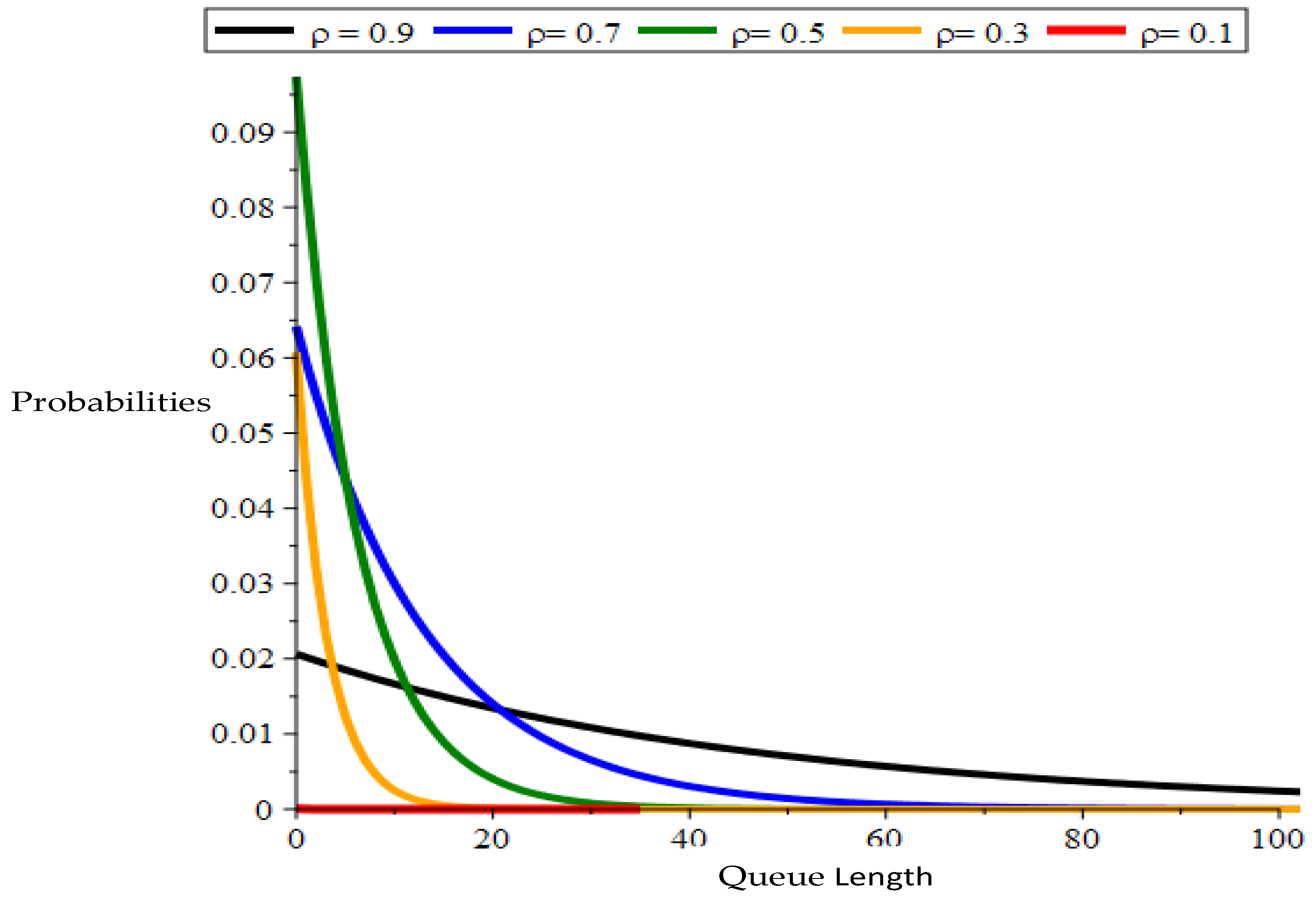
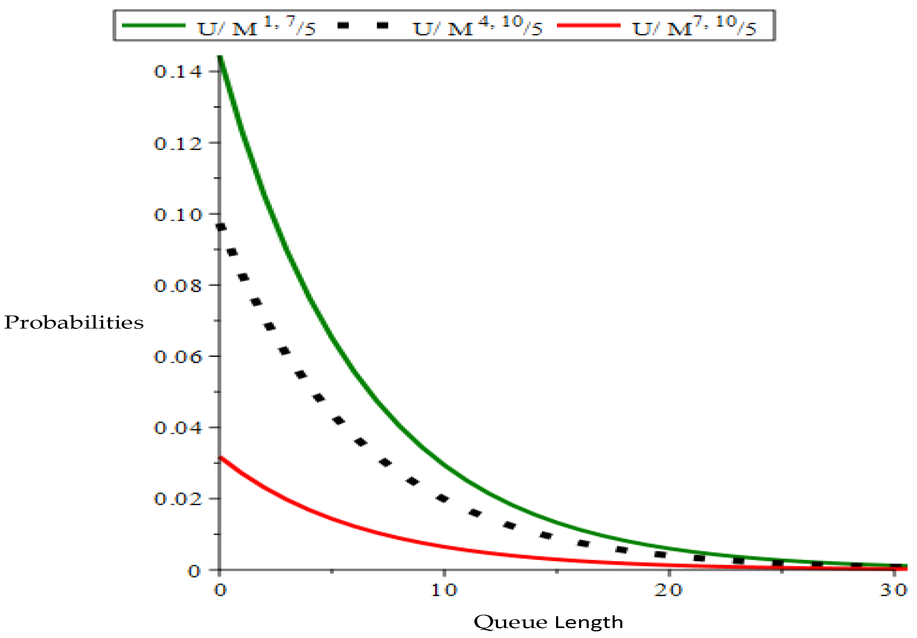
We considered three systems E6/Ma,10/5, D/Ma,10/5, and U/Ma,10/5 (. All three systems have the same mean value of inter-arrival time . In Table 8, we present the performance measures for these three systems for idle servers at three different epochs with varied and . In Figure 1, we compare the performance of D/M4,10/5 for busy servers at pre-arrival epochs with and . In Figure 2, we compare the performance of U/Ma,10/5 for busy servers at pre-arrival epochs with .
Table 8.
Comparison of performance measures of E6/Ma,10/5, D/Ma,10/5, and U/Ma,10/5 for idle servers, a = 1, 4, 7, = 0.1, 0.5, 0.9, = 10.
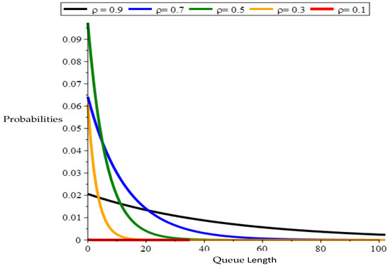
Figure 1.
Comparison of performance measures of D/M4,10/5 for busy servers, = 0.1, 0.3, 0.5, 0.7, 0.9, = 10.

Figure 2.
Comparison of performance measures of U/Ma,10/5 for busy servers, a = 1, 4, 7, = 0.5, = 10.
8. Conclusions
The queue GI/M/c was successfully investigated by using the two-dimensional embedded Markov chain. Simple and exact analyses to determine queue-length distributions are presented. An algorithm was derived for the analysis of the steady state behaviour of the system. Our recursive solution approach is not only very efficient, but also accurate by providing the exact queue-length probabilities at p.a.e. In a similar manner, we studied the queue-length distribution at r.e. and derived closed-form formulae in terms of the root w for evaluating the exact queue-length probabilities at r.e. We also obtained the probabilities of p.d.e. through the relations between r.e. and p.d.e. The results for this system were provided numerically by considering three inter-arrival time distributions—Erlang, deterministic, and uniform. The work on higher order moments and other distributions can be conducted similarly.
There are two special features in this work. The first is the effort to express the important results in closed form; the second is the development of the methodology and algorithms to efficiently derive accurate results. The models under consideration were validated by using MAPLE to obtain numerical results with sufficient accuracy and trivial computational costs.
Author Contributions
The results in this paper are based on J.G.’s Ph.D. thesis Chapter 3. Conceptualization, methodology, writing—review and editing, funding acquisition, J.G. and M.C.; software, validation, formal analysis, writing—original draft preparation, J.G.; resources, supervision, M.C. All authors have read and agreed to the published version of the manuscript.
Funding
This research was supported by the Royal Military College of Canada Professional Development Allocation.
Institutional Review Board Statement
Not applicable.
Informed Consent Statement
Not applicable.
Data Availability Statement
Not applicable.
Conflicts of Interest
The authors declare no conflict of interest.
Appendix A. Algorithm for Calculating p.a.e. Probabilities
The method for determining the complete solution to the stationary queue-length probabilities at p.a.e. for the model GI/M/c is described in the following steps:
- Find the unique real root w inside the unit circle of Equation (14).
- . Let
- Calculate by using Equation (20).
- Calculate by using Equation (19).
- Calculate recursively by using Equation (21).
- Substitute and into Equation (22) to find . Let .
- Repeat step 4 to step 6, and solve for the rest of the idle server probabilities.
- Finally, find the normalized p.a.e. vector using .
Appendix B. Proof of Equation (25)
Proof.
□
References
- Shyu, K. On the queueing processes in the system GI/M/n with bulk service. Acta. Math. Sin. 1960, 10, 182–189. [Google Scholar]
- Gross, D.; Shortle, J.; Thompson, J.; Harris, C. Fundamentals of Queueing Theory; John Wiley and Sons: Hoboken, NJ, USA, 2008. [Google Scholar]
- Neuts, M. A general class of bulk queues with Poisson input. Ann. Math. Stat. 1967, 38, 759–770. [Google Scholar] [CrossRef]
- Easton, G.; Chaudhry, M. The queueing system Ek/Ma,b/1 and its numerical analysis. Comput. Oper. Res. 1982, 9, 197–205. [Google Scholar] [CrossRef]
- Chaudhry, M.; Madill, B. Probabilities and some measures of efficiency in the queueing system GI/Ma,b/1. Selecta Statistica Canadiana 1987, 7, 53–75. [Google Scholar]
- Neuts, M. Matrix-Geometric Solution in Stochastic Models—An Algorithmic Approach; John Hopkins University Press: Baltimore, MD, USA, 1981. [Google Scholar]
- Sasikala, S.; Indhira, K. Bulk service queueing models—A survey. Int. J. Pure Appl. Math. 2016, 106, 43–56. [Google Scholar]
- Medhi, J. Further results on waiting time distribution in Poisson queue under a general bulk wervice rule. Cahiers du C.E.R.O. 1979, 21, 183–189. [Google Scholar]
- Sim, S.; Templeton, J. Steady state results for the M/Ma,b/c batch-service system. Eur. J. Oper. Res. 1985, 21, 260–267. [Google Scholar] [CrossRef]
- Sim, S. On Multi-Vehicle Transportation Systems with Queue-Dependent Dispatching Policies. Ph.D. Thesis, University of Toronto, Toronto, ON, Canada, 1982. [Google Scholar]
- Adan, I.; Resing, J.C. Multi-server batch-service systems. Stat. Neerl. 2000, 54, 202–220. [Google Scholar] [CrossRef]
- Goswami, V.; Samanta, S.; Vijaya Laximi, P.; Gupta, U. Analyzing a multiserver bulk-service finite-buffer queue. Appl. Math. Model. 2008, 32, 1797–1812. [Google Scholar] [CrossRef]
- Shyu, K. The waiting time distribution for the queueing processes in the system GI/M/n with bulk service. Acta. Math. Sin. 1964, 14, 796–808. [Google Scholar]
- Chaudhry, M.; Templeton, J. A First Course in Bulk Queues; John Wiley & Sons, Inc.: New York, NY, USA, 1983. [Google Scholar]
Publisher’s Note: MDPI stays neutral with regard to jurisdictional claims in published maps and institutional affiliations. |
© 2022 by the authors. Licensee MDPI, Basel, Switzerland. This article is an open access article distributed under the terms and conditions of the Creative Commons Attribution (CC BY) license (https://creativecommons.org/licenses/by/4.0/).