Article

Local H∞ Control for Continuous-Time T-S Fuzzy Systems via Generalized Non-Quadratic Lyapunov Functions

School of Information and Automation, Qilu University of Technology (Shandong Academy of Sciences), Jinan 250353, China
*
Author to whom correspondence should be addressed.
Mathematics 2022, 10(19), 3438; https://doi.org/10.3390/math10193438
Submission received: 30 July 2022 / Revised: 16 September 2022 / Accepted: 18 September 2022 / Published: 21 September 2022
(This article belongs to the Special Issue Dynamical Systems and System Analysis)

Abstract

:
This paper further develops a relaxed method to reduce conservatism in H feedback control for continuous-time T-S fuzzy systems via a generalized non-quadratic Lyapunov function. Different from the results of some exisiting works, the generalized H state feedback controller is designed. The relaxed stabilization conditions are obtained by applying Finsler’s lemma with the homogenous polynomial multipliers, and the H performance is acquired by solving an optimization problem. In addition, the proposed method could be expanded to handle other control problems for fuzzy systems. Two examples are given to show the validity of the proposed results.

1. Introduction

Owing to its better approximation properties, the Takagi–Sugeno (T-S) system [1] has attracted much attention from different communities. The system comprises a set of linear models and normalized membership functions (MFs).
The analysis and synthesis of fuzzy systems have been widely studied, such as stability analysis [2,3,4,5], observer design [6,7], filter [8,9,10], etc. Due to some limitations of the proposed methods in the existing results, researchers are seeking new methods to obtain better results, such as larger domain of attraction or stability region, and better H or H 2 performance. To reduce conservatism, many methods usually focus on the form of Lyapunov functions (LFs), the structure of slack variables and analysis of MFs and its derivatives.
Considering the drawbacks of common quadratic LFs, the complex LFs such as the fuzzy Lyapunov functions (FLFs) [11], the non-quadratic Lyapunov functions (NQLFs) [12], the line-integral FLFs [13], and homogeneous polynomial Lyapunov functions (HPLFs) [14], the homogeneous polynomial non-quadratic Lyapunov functions (HPNQLFs) [15] were proposed successively to further reduce the conservatism of stability conditions. For instance, Ref. [12] proposed new relaxed linear matrix inequality (LMI) conditions based on NQLFs. Ref. [14] first provided local asymptotic stability conditions and obtained different estimations of the attraction domain by using HPLFs. Ref. [15] gave the asymptotically necessary and sufficient stability conditions for discrete-time fuzzy systems via non-parallel distributed compensation law (NPDCL) with HPNQLFs. In addition, Ref. [12] designed an NPDCL to outperform previous results. By using the multi-indexed matrix approach, a homogeneous polynomial nonparallel distribution compensator (HPNQDC) was designed in [16], but the Lyapunov matrix used is linearly dependent on MFs. Ref. [17] further generalized previous HPNQDC and enlarged the stabilization region. Based on congruence transformation and Polya’s theorem, inner and outer slack variables were introduced in [18,19,20,21] to obtain a less conservative conclusion. Therefore, the design of a generalized control law for the local H performance of continuous-time T-S fuzzy system is worthy of investigation.
On the other hand, due to the general dependence of LFs on MFs, the time derivative of MFs (TDMFs) must be discussed in the proof process. Usually, there are several ways to deal with the TDMFs: (1) Assuming the upper or lower bounds of TDMF; (2) Finding LMI conditions to guarantee the upper bounds of TDMF hold; (3) Designing the line-integral FLFs; (4) Using a switching idea for the TDMFs. By exploring the upper bounds and properties of TDMFs, Ref. [22] proposed relaxed stability conditions. Considering the lower bounds of TDMF, Ref. [3] provided sufficient conditions to minimize the peak-to-peak level performance of the T-S fuzzy model. However, they overlooked the fact that the TDMFs involved x ˙ including the control law to be solved, which might be difficult to support in practice. Refs. [23,24,25] proposed the LMI conditions that guaranteed that the boundary of TDMF hold, but ignored disturbance. The line-integral FLFs designed in [13] could abstain from TDMFs, but the Lyapnov matrix structure had to be limited, which might bring about conservatism. Ref. [26] proposed a switching idea by discussing the property of TDMFs, while designing robust methods to commendably incorporate the boundary information of MFs is complex. Therefore, effective methods to manage the TDMFs remain to be explored.
From the above discussions, this paper considers the design of a generalized control law for local H control of continuous-time T-S fuzzy systems to further reduce the conservatism of existing results. The contributions of this paper are as follows:
(1)
The generalized NQLFs and NPCL depending on multi-index MFs are designed, including that found in [27] and double-fuzzy-summation in [20] as a special case, and more variables are introduced to reduce the conservatism.
(2)
The new LMIs conditions, which reduce the adjusted parameters to be calculated [7] and avoid redundant restrictions such as LFs matrices, slack variables in [23,28], are obtained to bound the time derivatives of MFs with disturbance.
(3)
The extended stabilization conditions for H performance are obtained by polynomial technology. As q increases, conservatism of obtained conditions will reduce, and the proposed method can be generalized to handle other cases, such as output feedback controller design [5], finite-time annular domain stability [29], mean-square strong stability [30].

2. Problem Statement and Preliminaries

2.1. The T-S Fuzzy System

The T-S fuzzy system (1) in C x ( C x = { x : | x i | θ x i , i = 1 , 2 , , n } ) can be obtained by applying the local approximation method.
x ˙ ( t ) = i = 1 r h i ( x ( t ) ) ( A i x ( t ) + B 1 i ω ( t ) + B 2 i u ( t ) ) = A h x ( t ) + B 1 h ω ( t ) + B 2 h u ( t ) , z ( t ) = i = 1 r h i ( x ( t ) ) ( C 1 i x ( t ) + D 1 i ω ( t ) + D 2 i u ( t ) ) = C 1 h x ( t ) + D 1 h ω ( t ) + D 2 h u ( t ) , y ( t ) = i = 1 r h i ( x ( t ) ) C 2 i x ( t ) = C 2 h x ( t ) .
where the state x ( t ) R n × 1 , the measured output y ( t ) R n y × 1 , the external disturbance ω ( t ) R n w × 1 , the control input u ( t ) R n u × 1 and the controlled output z ( t ) R n z × 1 . A i R n × n , B 1 i R n × n ω , B 2 i R n × n u , C 1 i R n z × n , C 2 i R n y × n , D 1 i R n z × n ω , D 2 i R n z × n u and D 3 i R n y × n ω . h i ( x ) is the normalised MF satisfying i = 1 r h i ( x ( t ) ) = 1 .
The objective of this paper is to design a controller u ( t ) such that the system (1) with ω = 0 is locally asymptotically stable, and guarantees 0 t z ( t ) T z ( t ) d t γ 2 0 t ω ( t ) T ω ( t ) d t ( t > 0 ) under zero initial conditions.

2.2. Notations and Properties

N denotes the natural numbers set. n ! denotes factorial, i.e., n ! = n ( n 1 ) ( 2 ) ( 1 ) for n N with 0 ! = 1 . For any Φ R n × n , H e ( Φ ) = Φ + Φ T . x ( t ) , h ( x ( t ) ) are replaced, respectively, by x, h for convenience. Ω h = i = 1 r h i Ω i , Ω h h = i = 1 r j = 1 r h i h j Ω i j . d i a g { a 1 , , a n } = a 1 0 0 a n .
Based on the multi-index notations proposed in [19], that is, I q = { i q = ( i 1 , i 2 , , i q ) N q 1 i k r } , I q + = { i q I q i 1 i 2 i q } .
The notation of i q / i k ( i q I q + , 1 k r ) in [31] is recommended as follows:
i q / i k = i 1 i k 1 i k + 1 i p , if i k i q ; 0 , otherwise .
For instance, if i 1 i 2 i 2 I 3 + , k { 1 , 2 , 3 , 4 } , i 1 , i 2 i 3 , i 1 , i 2 i 4 , then i 1 i 2 i 2 / i 1 = i 2 i 2 , i 1 i 2 i 2 / i 2 = i 1 i 2 , i 1 i 2 i 2 / i 3 = 0 , i 1 i 2 i 2 / i 4 = 0 .
The form of MFs for a product is expressed:
h i q = l = 1 q h i l = h i 1 h i 2 h i q = h 1 q 1 h 2 q 2 h r q r ,
where i = 1 r q i = q .
According to the convex sum property of MFs, one has
1 = i = 1 r h i = ( i = 1 r h i ) q = i q I q + g i q h i q ,
where g i q = q ! q 1 ! q 2 ! q r ! , i = 1 r q i = q . For example, as r = 2 , q = 4 , if i 1 = i 2 = 1 , i 3 = i 4 = 2 , h 1 h 1 h 2 h 2 = h 1 2 h 2 2 or i 1 = 1 , i 2 = i 3 = i 4 = 2 , h 1 h 2 h 2 h 2 = h 1 h 2 3 , one gets g 1122 = 4 ! 2 ! 2 ! = 6 ( q 1 = 2 , q 2 = 2 ) or g 1222 = 4 ! 1 ! 3 ! = 4 ( q 1 = 1 , q 2 = 3 ).
The q-dimensional fuzzy summations of matrices are defined as follows:
Ω h = i q I q h i q Ω i q = i 1 = 1 r i q = 1 r h i 1 h i q Ω i 1 i q Ω h + = i q I q + h i q Ω i q = i 1 = 1 r i q = i q 1 r h i 1 h i q Ω i 1 i q
To facilitate the formula derivation, the following lemma and several properties are cited.
Lemma 1 (Finsler’s Lemma [18]).
Let ζ R n , Θ R n × n , Φ R m × n , r a n k ( Φ ) < n , then ζ T Θ ξ < 0 , ζ 0 , such that Φ ζ = 0 , if and only if one of the following conditions holds:
(1)
Φ T Θ Φ < 0 , where Φ satisfies Φ Φ = 0 , and Φ Φ T + Φ T Φ > 0 ;
(2)
μ R : Θ μ Φ T Φ < 0 ;
(3)
V R m × n : Θ + V Φ + Φ T V T < 0 .
Property 1 ([18]).
The following inequalities are equivalent:
(1)
Find symmetric matrix X = X T , such that T + A T X T + X A < 0 .
(2)
Find symmetric matrix X = X T , R 1 , R 2 , such that
T + A T R 1 T + R 1 A ( * ) X R 1 T + X T A R 2 R 2 T < 0 .
Property 2 ([32]).
Considering matrices Φ = Φ T and Ψ = Ψ T with suitable dimensions, if Φ + μ Ψ < 0 and Φ μ Ψ < 0 , then Φ + h ˙ Ψ < 0 holds for any h ˙ and μ satisfying | h ˙ | μ ( μ > 0 ) .
Property 3 ([19]).
Let Ω i q , i q I q + be the matrices of proper dimensions. Then, Ω h q < 0 holds if
Ω i q < 0 .

3. Main Results

Theorem 1.
If given μ j > 0 , h j x σ j , j I 1 , ω δ , there exist symmetric matrices P i q > 0 , ( i q I q ) and M i q + 1 ( i q + 1 I q + 1 + ), matrices F i q , L i q l 1 l 2 and G i q l 1 l 2 ( i q I q + ) ( l 1 , l 2 = 1 , 2 , 3 ), such that
Ω i q + 1 ( 1 ) = Ω 11 Ω 12 Ω 13 Ω 14 Ω 15 Ω 16 Ω 22 Ω 23 Ω 24 Ω 25 Ω 26 Ω 33 Ω 34 Ω 35 Ω 36 Ω 44 Ω 45 Ω 46 Ω 55 Ω 56 Ω 66 < 0 ,
Ω i q + 1 ( 2 ) = i = 1 r P P ( i q + 1 / i k ) 0 ( ) 0 I ( ) i k = 1 q ( ε x A i k P i ¯ + ε x B 2 i k F i ¯ ) B 1 i k g i q + 1 α 2 μ j 2 ρ σ j 2 > 0 ,
where i ¯ = i q + 1 / i k ,
Ω 11 = i k = 1 q H e ( L i ¯ 11 A i k T + B 2 i k F i ¯ ) ± j = 1 r μ j Ω ¯ i q + 1 j , Ω ¯ i q + 1 j = j = 1 r j q P ( i q + 1 / j ) ( P j j q + + P j 1 j ) + M i q + 1 , Ω 12 = i k = 1 q ( g i ¯ B 1 i k + A i k L i ¯ 21 T ) , Ω 13 = i k = 1 q ( F i ¯ T D 2 i k T + L i ¯ 11 C 1 i k T + A i k L i ¯ 31 T ) , Ω 14 = i k = 1 q ( P P ( i ¯ ) L i ¯ 11 + A i k G i ¯ k 11 ) , Ω 15 = i k = 1 q ( L i ¯ 12 + A i k G i ¯ 12 ) , Ω 16 = i k = 1 q ( L i ¯ 13 + A i k G i ¯ 13 ) , Ω 22 = g i q + 1 γ 2 , Ω 23 = i k = 1 q ( D 1 i k T + L i ¯ 21 C 1 i k T ) , Ω 24 = i k = 1 q L i ¯ 21 , Ω 25 = g i q + 1 I i k = 1 q L i ¯ 22 , Ω 26 = i k = 1 q L i ¯ 23 , Ω 33 = i k = 1 q H e ( L i ¯ 31 C 1 i k T ) g i q + 1 I , Ω 34 = i k = 1 q ( L i ¯ 31 + C 1 i k G i ¯ 11 ) , Ω 35 = i k = 1 q ( L i ¯ 32 + C 1 i k G i ¯ 12 ) , Ω 36 = g i q + 1 I i k = 1 q ( L i ¯ 33 + C 1 i k G i ¯ 13 ) , Ω 44 = i k = 1 q H e ( G i ¯ 11 ) , Ω 45 = i k = 1 q ( G i ¯ 12 G i ¯ 21 T ) , Ω 46 = i k = 1 q ( G i ¯ 13 G i ¯ 31 T ) , Ω 55 = i k = 1 q H e ( G i ¯ 22 ) , Ω 56 = i k = 1 q ( G i ¯ 23 G i ¯ 32 T ) , Ω 66 = i k = 1 q H e ( G i ¯ 33 ) .
then, the closed-loop system (1) in Ω x ( : = { x : x T P h q 1 x ρ } ) is locally asymptotically stable with a disturbance attenuation level γ under the controller (9)
u ( t ) = F h q + P h q 1 x .
Proof. 
Designing the generalized NQLF candidate as
V ( x ) = x T P h q 1 x ,
and letting Γ = V ˙ ( x ) + z T z γ 2 ω T ω , we get
Γ = η T Λ 1 P 1 B 1 h + C ¯ T D 1 h ( ) γ 2 + D 1 h T D 1 h η ,
where Λ 1 = H e ( P h q 1 A ¯ ) + P ˙ h q 1 + C ¯ T C ¯ , η T = x T ω T , A ¯ = A h + B 2 h F h q + P h q 1 , C ¯ = C 1 h + D 2 h F h q + P h q 1 . □
On one hand, Γ 0 is guaranteed by the following formula:
H e ( P h q 1 A ¯ ) + P ˙ h q 1 P h q 1 B 1 h C ¯ B 1 h T P h q 1 γ 2 D 1 h T C ¯ D 1 h I < 0 .
Multiplying left and right by d i a g { P h q , I , I } and using the relation P ˙ h q 1 = P h q 1 P ˙ h q P h q 1 , Equation (12) is transformed into
H e ( A ¯ P h q ) P ˙ h q B 1 h P h q C ¯ B 1 h T γ 2 D 1 h T C ¯ P h q D 1 h I < 0 .
Starting from the characteristics where j = 1 r h ˙ j = 0 , thus j = 1 r h ˙ j M h q + 1 + = 0 for any symmetric matrix M h q + 1 + with suitable size, adding j = 1 r h ˙ j M h q + 1 + to (13) and using Property 2, we get
H e ( A ¯ P h q ) ± Ω j B 1 h P h q C ¯ T B 1 h T γ 2 D 1 h T C ¯ P h q D 1 h I < 0 ,
where Ω j = j = 1 r h ˙ j ( P h q j + M h q + 1 + ) .
Then, Equation (14) is transformed in to
Q + Λ 2 T P ^ + P ^ Λ 2 < 0
where
Q = H e ( B 2 h F h q + ) Ω B 1 h ( F h q + ) T D 2 h T γ 2 D 1 h T I , P ^ = P h q 0 0 0 I 0 0 0 I , Λ 2 T = A h 0 0 0 0 0 C 1 h 0 0 .
Applying Property 1 to (15), one gets
Ω h q + 1 = Ω ¯ 11 Ω ¯ 12 Ω ¯ 13 Ω ¯ 14 Ω ¯ 15 Ω ¯ 16 γ 2 Ω ¯ 23 Ω ¯ 24 Ω ¯ 25 Ω ¯ 26 Ω ¯ 33 Ω ¯ 34 Ω ¯ 35 Ω ¯ 36 Ω ¯ 44 Ω ¯ 45 Ω ¯ 46 Ω ¯ 55 Ω ¯ 56 Ω ¯ 66 < 0 ,
where
Ω ¯ 11 = H e ( L h q + 11 A h T + B 2 h F h q + ) ± Ω j , Ω ¯ 12 = B 1 h + A h L h q + 21 T , Ω ¯ 13 = F h q + T D 2 h T + L h q + 11 C 1 h T + A h L h q + 31 T , Ω ¯ 14 = P h q L h q + 11 + A h G h q + 11 , Ω ¯ 15 = L h q + 12 + A h G h q + 12 , Ω ¯ 16 = L h q + 13 + A h G h q 13 , Ω ¯ 23 = D 1 h T + L h q + 21 C 1 h T , Ω ¯ 24 = L h q + 21 , Ω ¯ 25 = I L h q + 22 , Ω ¯ 26 = L h q + 23 , Ω ¯ 33 = I + H e ( L h q + 31 C 1 h T ) , Ω ¯ 34 = L h q + 31 + C 1 h G h q + 11 , Ω ¯ 35 = L h q + 32 + C 1 h G h q + 12 , Ω ¯ 36 = I L h q + 33 + C 1 h G h q + 13 , Ω ¯ 44 = H e ( G h q + 11 ) , Ω ¯ 45 = G h q + 12 G h q + 21 T , Ω ¯ 46 = G h q + 13 G h q + 31 T , Ω ¯ 55 = H e ( G h q + 22 ) , Ω ¯ 56 = G h q + 23 G h q + 32 T . Ω ¯ 66 = H e ( G h q + 33 ) ,
According to Property 2, (16) is warranted by (7) with | h ˙ j | μ j .
On the other hand, we discuss | h ˙ j | μ j . Let
| h ˙ j | = | ( h j x ) T ε x ( A h x + B 2 h F h q + P h q 1 x + B 1 h ω ) | μ j .
Notation: If h contains all state x, then ε x is the unit matrix. If h only contains a part of state, for instance, x = [ x 1 , x 2 , x 3 , x 4 ] T , h depends on x 1 , x 3 , then ε x = d i a g { 1 , 0 , 1 , 0 } .
For (17), one has
η T Δ T h j x ( h j x ) T Δ η < μ j 2 ,
where Δ = ε x [ A h + B 2 h F h q + P h q 1 , B 1 h ] , η = [ x ; ω ] .
It is known that ( h j x ) T h j x σ j 2 h j x ( h j x ) T σ j 2 I and η T d i a g { P h q 1 , I } η ρ + δ 2 . Equation (18) is guaranteed by
( ρ + δ 2 ) σ j 2 α 2 μ j 2 Δ T Δ d i a g { P h q 1 , I } < 0 ,
Utilizing Schur complement to (19) and multiplying left and right by d i a g { P h q , I } , one has
P h q 0 I ε x ( A h P h q + B 2 h F h q + ) B 1 h α 2 μ j 2 ρ σ j 2 > 0 .
Therefore, if (7) and (8) hold, we have Γ < 0 , which means 0 z T z d t γ 2 0 ω T ω d t . The proof is completed.
Remark 1.
TDMFs in [20,23] were bounded without disturbance and some assumed conditions such as matrix P ( P i > λ x 2 + λ k 2 2 β k I ) and the free variable S ( S h = P h ) in [28,33] were limited. This paper eliminates these restrictions or assumptions.
Remark 2.
Due to ( h j x ) T h j x σ j 2 being restricted, Theorem 1 means a local result. The Lyapunov level Ω x ( x T P h q 1 x ρ ) is an estimated region for H performance, which must be contained in Θ x . Applying the Lagrange multiplier method, we get
λ x i 2 ρ e i P h q P h q e i T P h q 0
Thus, according to Property 3, conditions (22) guarantee (21).
g i q λ x i 2 ρ e i P P ( i q ) P P ( i q ) 0 , i = 1 , 2 , , n
Remark 3.
There are two parameters μ j and ρ in Theorem 1 to be searched. By solving the following optimization problem, one can get H performance with given μ j and ρ.
m i n P P ( i q ) > 0 , F i q , L i q , G i q , μ j , α γ s . t . ( 7 ) , ( 8 ) , ( 22 )
Compared with the methods in [28,33], if | h ˙ j | μ j is decomposed, that is,
| ( h j x ) T ε x ( A h + B 2 h F h q + P h q 1 ) x | α μ j
| ( h j x ) T ε x B 1 h ω | ( 1 α ) μ j
then (8) will be substituted with (26) and (27).
Corollary 1.
Given μ j > 0 , h j x σ j , j I 1 , ω δ , α ( 0 , 1 ) , if (7), (26), (27) and (22) hold,
Ω i q + 1 ( 2 ) = i = 1 r P P ( i q + 1 / i ) ( ) Ω 21 ( 2 ) g i q + 1 α 2 μ j 2 ρ σ j 2 > 0 ,
( 1 α ) 2 μ j 2 δ 2 ( ) ε x B 1 i k 1 σ j 2 > 0 ,
Then, the closed-loop system (1) in Ω x ( : = { x : x T P h q 1 x ρ } ) is locally asymptotically stable with a disturbance attenuation level γ under the controller (9).
Proof. 
The proof is similar to that of Theorem 1, and is thus omitted here. □

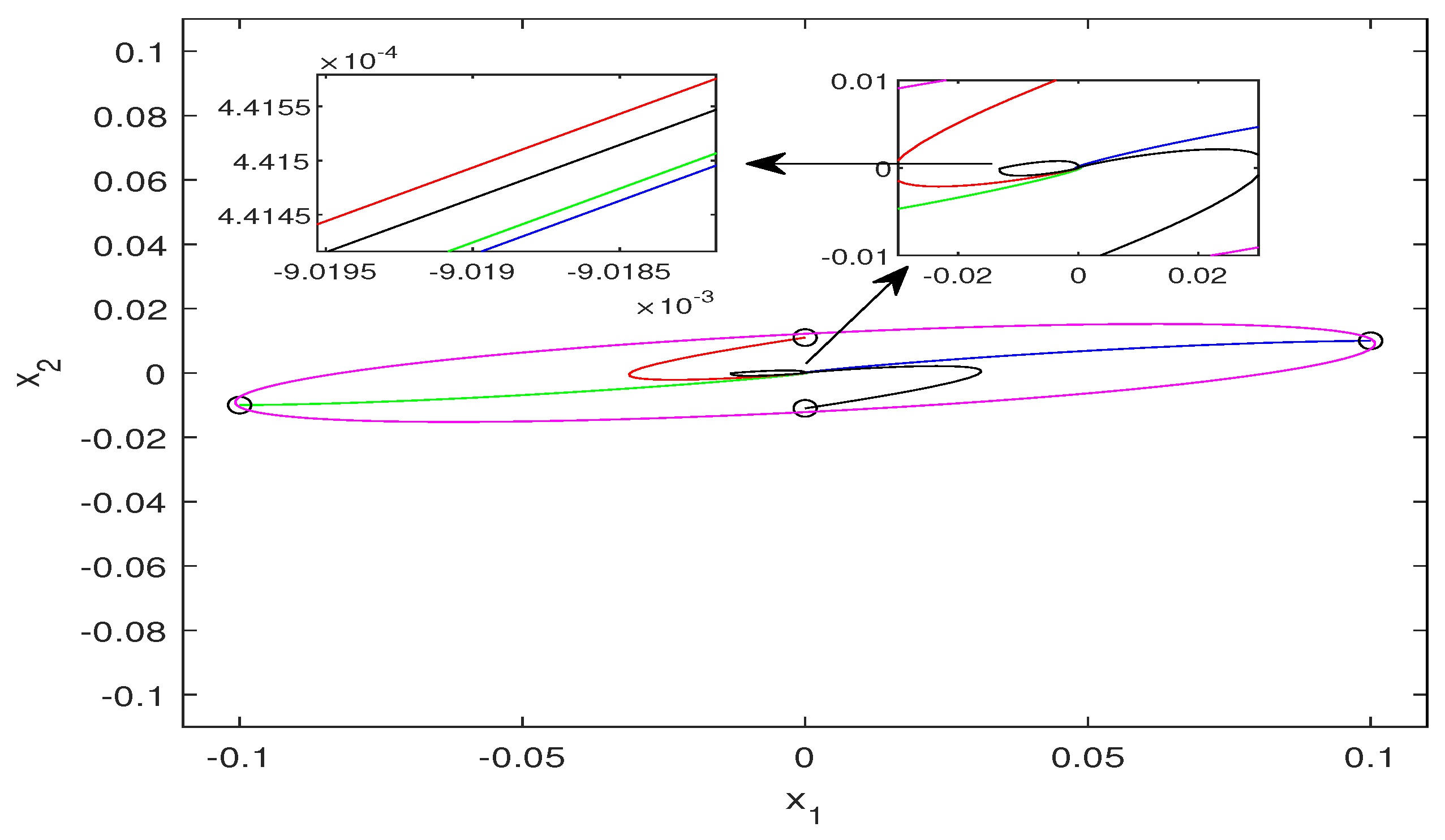
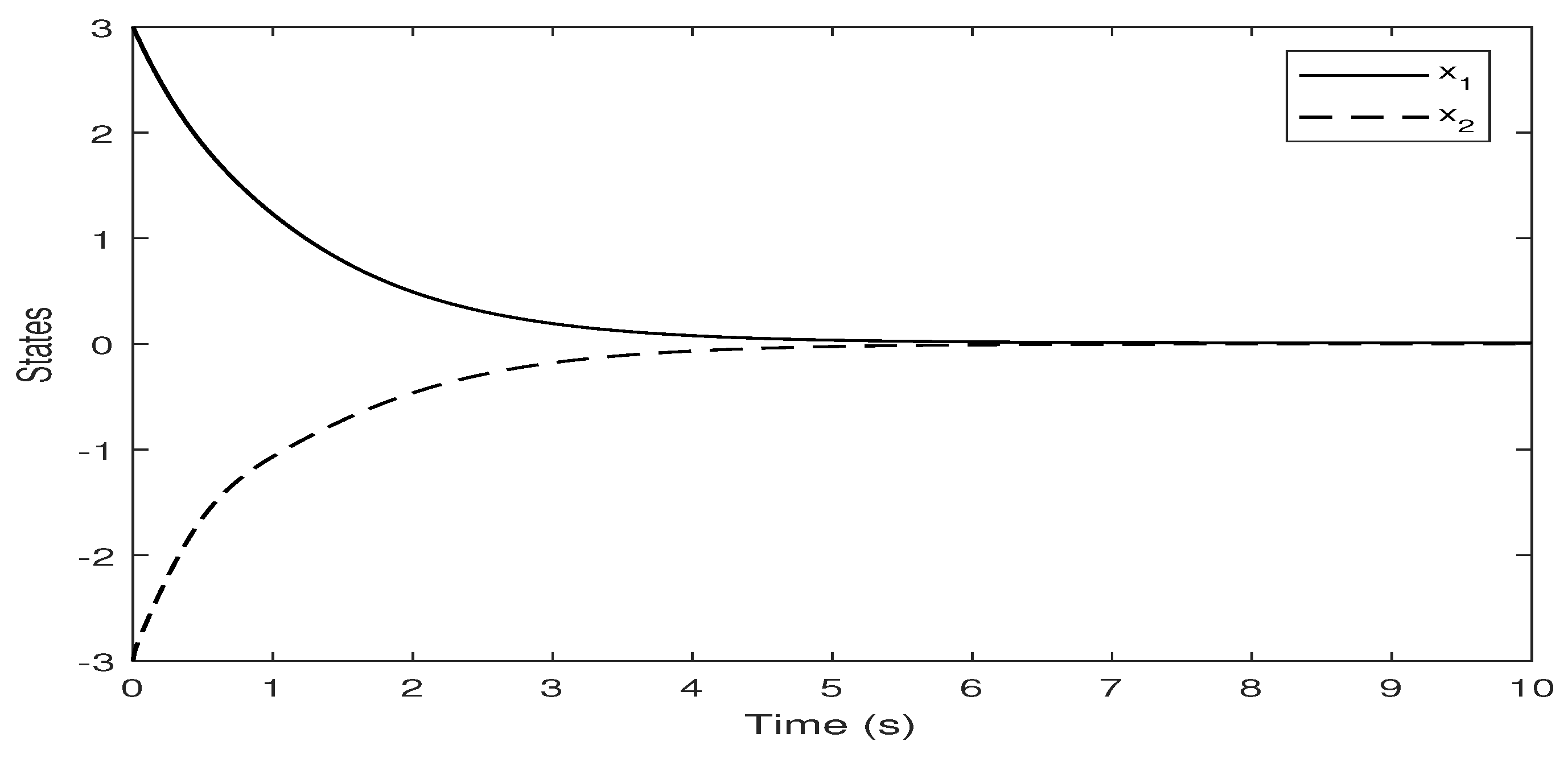
4. Simulation Example

All the experiments were performed on a computer with an Intel(R) Core(TM)i5-7200U CPU @ 2.50 GHz 2.70 GHz, 12 GB(RAM), using Matlab2017a.
Example 1.
Considering the following nonlinear system form [33].
x ˙ 1 = 6 x 1 4.33 x 2 + 7.59 x 1 s i n 2 ( x 1 ) 2.96 x 2 s i n 2 ( x 1 ) + ( s i n 2 ( x 1 ) 2.06 c o s 2 ( x 1 ) ) u + ( 0.1 + 0.01 c o s 2 ( x 1 ) ) ω x ˙ 2 = x 1 s i n 2 ( x 1 ) + 5 x 2 5 s i n 2 ( x 1 ) x 2 c o s 2 ( x 1 ) u + ( 0.01 s i n 2 ( x 1 ) + 0.03 ) ω
The above system is expressed as a T-S fuzzy system with two rules in the C x = { x : | x i | π 2 , i = 1 , 2 } . One gets the system matrices:
A 1 = 1.59 7.29 1 0 , A 2 = 6 4.33 0 5 , B 11 = 0.01 0.04 , B 12 = 0.011 0.03 , B 21 = 1 0 , B 22 = 2.06 1 , C 11 = C 12 = 1 2 , D 11 = D 12 = D 21 = D 22 = 0 , h 1 = s i n 2 ( x 1 ) , h 2 = 1 h 1 .
Since h 1 x = 2 s i n ( x 1 ) c o s ( x 1 ) and h 2 x = 2 s i n ( x 1 ) c o s ( x 1 ) , thus
( h 1 x ) T h 1 x 1 , ( h 2 x ) T h 2 x 1 ,
one has σ i 2 = 1 .
The external disturbance signal ω ( t ) = { s i n ( t ) , 5 t 15   s 0 , else . The parameters required by Theorem 1 in the region Ω x ( x T P h q 1 x ρ = 1 ) are as follows: σ i 2 = 1 , λ x i 2 = π 2 4 , δ 2 = 1 , μ i = 1000 .
All results are solved by function m i n x in Matlab Toolbox. The minimal γ obtained are shown in Table 1 under different methods. Notice, a line indicates that SeDuMi solver is unable to converge to a solution.
This clearly shows that the Theorem 1 proposed in this paper is less conservative than other methods. Moreover, as q increases, better results are obtained.
On the other hand, when systems include unknown parameters, such as B 22 = 2.06 + λ 1 , we compare the minimal γ with the different λ shown in Table 2. Although the minimal γ increases with the parameter λ , Theorem 1’s results are better than other ones under the same parameter λ .
When λ = 1 and q = 3 , one gets γ = 0.0259 and the gain matrices as follow.
P 111 = 1.4172 1.3062 1.3062 1.2039 , F 111 = 13.5716 10.4026 T , P 112 = 0.0001 0.0044 0.0044 1.4004 , F 112 = 48.4813 22.6372 T , P 122 = 7.0579 3.9604 3.9604 2.2224 , F 122 = 51.1398 55.7751 T , P 222 = 2.4673 1.0802 1.0802 0.4736 , F 222 = 3.3849 5.5163 T .
Choosing the initial four points
x 0 ( 1 ) = 0.1 0.01 T , x 0 ( 2 ) = 0.1 0.01 T , x 0 ( 3 ) = 0 0.011 T , x 0 ( 4 ) = 0 0.011 T ,
four trajectory curves in the domain of attraction Ω x are shown in Figure 1, which are asymptotically driven to the origin under the controller. Therefore, this shows that the designed controller is effective.
Example 2.
The state equation of motion for the inverted pendulum controlled by a separately excited direct current (DC) motor from [35].
x ˙ 1 ( t ) = x 2 ( t ) , x ˙ 2 ( t ) = g l s i n x 1 ( t ) + N K 1 m l 2 x 3 ( t ) + ω , 0 = N K 2 x 2 ( t ) R ¯ x 3 ( t ) + u ,
where x 1 [ π π ] denotes the angle, x 2 denotes the angular velocity, x 3 represents the current of the DC motor, u is the control input voltage. The parameter values of the system are m = 1 kg, l = 1 m, g = 9.8 m/s2, N = 10 , K 2 = 0.1 Vs/rad, K 1 = 0.1 Nm/A and 0.6 Ω R ¯ 3.5 Ω .
Equation (29) can be converted to
x ˙ 1 ( t ) = x 2 ( t ) , x ˙ 2 ( t ) = g l s i n x 1 ( t ) N 2 K 1 K 2 m l 2 R ¯ x 2 ( t ) + N K 1 m l 2 R ¯ u + ω .
We consider z = x 1 + x 2 . Applying local approximation method, the T-S fuzzy model (1) is given with A 1 = 0 1 9.8 5 3 , A 2 = 0 1 0 5 3 , B 21 = 0 5 3 , B 22 = 0 5 3 , B 11 = 0 1 , B 12 = 0 1 , C 11 = 1 1 , C 12 = 1 1 , D 11 = D 12 = D 21 = D 22 = 0 . h 1 = s i n ( x 1 ) + 1 2 , h 2 = 1 h 1 defined in the compact set C = { x : | x 1 | π , | x 2 | π } .
Since h 1 x = c o s ( x 1 ) 2 0 T and h 2 x = c o s ( x 1 ) 2 0 T , thus ( h 1 x ) T h 1 x 1 4 , ( h 2 x ) T h 2 x 1 4 , one has μ i 2 = 1 4 . Selecting σ i 2 = 1 4 , λ x 2 = 2 π 2 , ρ = 1 .
Here, we consider that the derivative of MFs ( μ 1 = μ 2 ) in Theorem 1 affects the conservativeness of the different method. The results are shown in Table 3. It can be seen that [23,27,33] cannot converge to a solution when μ = 1 , but Theorem 1 can. Moreover, as μ i increases, γ decreases, and Theorem 1’s results with q = 2 are better than other ones under the same parameter μ .
Choosing q = 2 , μ = 100 , we get γ = 6.3759 × 10 6 and control gain matrixes as follow:
P 11 = 10 6 × 6.8474 6.7747 6.7747 6.8257 , F 11 = 10 5 × 5.6759 6.5064 T , P 12 = 10 6 × 7.1174 6.9996 6.9996 7.0022 , F 12 = 10 6 × 0.5910 9.8859 T , P 22 = 10 6 × 6.9380 6.8626 6.8626 6.9128 , F 22 = 10 6 × 0.0242 7.6379 T .
From the starting point x 0 = [ 3 , 3 ] T , the response trajectories of the states, Lyapunov function and control input are shown in Figure 2, Figure 3 and Figure 4, respectively. Therefore, the closed-loop system (30) is locally asymptotically stable with disturbance attenuation level γ under the controller (9).

5. Conclusions

This paper has presented the local H control for continuous-time T-S fuzzy systems via generalized nonquadratic Lyapunov functions. Using polynomial technology, relaxed LMIs conditions satisfying H performance are obtained, which are easily solved by the optimization problem. The simulation examples provided show the validity of the proposed method.
Furthermore, the method proposed in this paper could be generalized to handle problems regarding output feedback controllers, filters or observers. Now, our group is considering the output feedback controller design for nonlinear systems, finite-time boundedness, finite-time annular domain stability and mean-square strong stability for stochastic systems using our method.

Author Contributions

Formal analysis, Z.Y. and G.H.; methodology, G.H.; funding acquisition, Z.Y.; investigation, software, and writing—original draft preparation and editing, J.Z.; review and editing, Z.Y. and G.H. All authors have read and agreed to the published version of the manuscript.

Funding

This paper is supported in part by the National Natural Science Foundation of China under Grants (61877062, 61977043).

Institutional Review Board Statement

Not applicable.

Informed Consent Statement

Not applicable.

Data Availability Statement

Not applicable.

Conflicts of Interest

The authors declare no conflict of interest.

References

  1. Takagi, T.; Sugeno, M. Fuzzy identification of systems and its applications to modeling and control. IEEE Trans. Syst. Man Cybern. 1985, 15, 387–403. [Google Scholar] [CrossRef]
  2. Su, X.J.; Wu, L.G.; Shi, P.; Song, Y.D. A novel approach to output feedback control of fuzzy stochastic systems. Automatica 2014, 50, 3268–3275. [Google Scholar] [CrossRef]
  3. Vafamand, N.; Asemani, M.H.; Khayatiyan, A.; Khooban, M.H.; Dragicevic, T. TS Fuzzy Model-Based Controller Design for a Class of Nonlinear Systems Including Nonsmooth Functions. IEEE Trans. Syst. Man Cybern. Syst. 2020, 50, 233–244. [Google Scholar] [CrossRef]
  4. Achour, H.; Boukhetala, D.; Labdelaoui, H. An observer-based robust H∞ controller design for uncertain Takagi-Sugeno fuzzy systems with unknown premise variables using particle swarm optimisation. Int. J. Syst. Sci. 2020, 51, 2563–2581. [Google Scholar] [CrossRef]
  5. Yan, Z.; Zhang, J.; Hu, G. A new approach to fuzzy output feedback controller design of continuous-time Takagi-Sugeno fuzzy systems. Int. J. Fuzzy Syst. 2020, 22, 2223–2235. [Google Scholar] [CrossRef]
  6. Chang, X.H.; Yang, G.H.; Wang, H. Observer-based H∞ control for discrete-time T-S fuzzy systems. Int. J. Syst. Sci. 2011, 42, 1801–1809. [Google Scholar] [CrossRef]
  7. Wang, L.K.; Zhang, H.G.; Liu, X.D. H∞ Observer Design for Continuous-Time Takagi-Sugeno Fuzzy Model with Unknown Premise Variables via Nonquadratic Lyapunov Function. IEEE Trans. Cybern. 2016, 46, 1986–1996. [Google Scholar] [CrossRef]
  8. Zhang, Z.; Lin, C.; Chen, B. New decentralized H∞ filter design for nonlinear interconnected systems based on Takagi-Sugeno fuzzy models. IEEE Trans. Cybern. 2015, 45, 2914–2924. [Google Scholar] [CrossRef] [PubMed]
  9. Shi, P.; Su, X.; Li, F. Dissipativity-based filtering for fuzzy switched systems with stochastic perturbation. IEEE Trans. Autom. Control 2016, 61, 1694–1699. [Google Scholar] [CrossRef]
  10. Dong, J.; Yang, G. H∞ Filtering for Continuous-Time T-S Fuzzy Systems with Partly Immeasurable Premise Variables. IEEE Trans. Syst. Man Cybern. Syst. 2017, 47, 1931–1940. [Google Scholar] [CrossRef]
  11. Tanaka, K.; Hori, T.; Wang, H.O. A multiple Lyapunov function approach to stabilization of fuzzy control systems. IEEE Trans. Fuzzy Syst. 2003, 11, 582–589. [Google Scholar] [CrossRef]
  12. Guerra, T.M.; Vermeiren, L. LMI-based relaxed nonquadratic stabilization conditions for nonlinear systems in the Takagi-Sugeno’s form. Automatica 2004, 40, 823–829. [Google Scholar] [CrossRef]
  13. Rhee, B.J.; Won, S. A new fuzzy Lyapunov function approach for a Takagi-Sugeno fuzzy control system design. Fuzzy Sets Syst. 2006, 157, 1211–1228. [Google Scholar] [CrossRef]
  14. Bernal, M.; Guerra, T.M. Generalized nonquadratic stability of continuous-time Takagi-Sugeno models. IEEE Trans. Fuzzy Syst. 2010, 18, 815–822. [Google Scholar] [CrossRef]
  15. Ding, B. Homogeneous polynomially nonquadratic stabilization of discrete-time Takagi-Sugeno systems via nonparallel distributed compensation law. IEEE Trans. Fuzzy Syst. 2010, 18, 994–1000. [Google Scholar] [CrossRef]
  16. Zhang, H.; Xie, X. Relaxed stability conditions for continuous-time T-S fuzzy-control systems via augmented multi-indexed matrix approach. IEEE Trans. Fuzzy Syst. 2011, 19, 478–492. [Google Scholar] [CrossRef]
  17. Hu, G.; Liu, X.; Wang, L.; Li, H. Relaxed stability and stabilisation conditions for continuous-time Takagi-Sugeno fuzzy systems using multiple-parameterised approach. IET Control Theory Appl. 2017, 11, 774–780. [Google Scholar] [CrossRef]
  18. Delmotte, F.; Guerra, T.M.; Ksantini, M. Continuous Takagi-Sugeno’s models: Reduction of the number of LMI conditions in various fuzzy control design technics. IEEE Trans. Fuzzy Syst. 2007, 15, 426–438. [Google Scholar] [CrossRef]
  19. Sala, A.; Arino, C. Asymptotically necessary and sufficient conditions for stability and performance in fuzzy control: Applications of Polya’s theorem. Fuzzy Sets Syst. 2007, 158, 2671–2686. [Google Scholar] [CrossRef]
  20. Vafamand, N.; Khooban, M.H.; Khayatian, A.; Blaabjerg, F. Design of Robust Double-Fuzzy-Summation Non-PDC Controller for Chaotic Power Systems. J. Dyn. Syst. Meas. Control 2018, 140, 031004. [Google Scholar] [CrossRef]
  21. Wang, L.; Lam, H. H∞ control for continuous-time Takagi-Sugeno fuzzy model by applying generalized Lyapunov function and introducing outer variables. Automatica 2021, 125, 109409. [Google Scholar] [CrossRef]
  22. Faria, F.A.; Silva, G.N.; Oliveira, V.A. Reducing the conservatism of LMI-based stabilisation conditions for T-S fuzzy systems using fuzzy Lyapunov functions. Int. J. Syst. Sci. 2013, 44, 1956–1969. [Google Scholar] [CrossRef]
  23. Pan, J.; Guerra, T.M.; Fei, S.; Jaadari, A. Nonquadratic stabilization of continuous T-S fuzzy models: LMI solution for a local approach. IEEE Trans. Fuzzy Syst. 2012, 20, 594–602. [Google Scholar] [CrossRef]
  24. Marquez, R.; Guerra, T.M.; Bernal, M.; Kruszewski, A. Asymptotically necessary and sufficient conditions for Takagi-Sugeno models using generalized non-quadratic parameter-dependent controller design. Fuzzy Sets Syst. 2017, 306, 48–62. [Google Scholar] [CrossRef]
  25. Vafamand, N.; Asemani, M.H.; Khayatian, A. Robust L1 Observer-based Non-PDC Controller Design for Persistent Bounded Disturbed TS Fuzzy Systems. IEEE Trans. Fuzzy Syst. 2017, 26, 1401–1413. [Google Scholar] [CrossRef]
  26. Wang, L.; Liu, J.; Lam, H.K. Further study on stabilization for continuous-time Takagi-Sugeno fuzzy systems with time delay. IEEE Trans. Cybern. 2021, 51, 5637–5643. [Google Scholar] [CrossRef]
  27. Hu, G.; Wang, L.; Liu, X. A new approach to local H∞ control for continuous-time T-S fuzzy models. J. Intell. Fuzzy Syst. 2020, 39, 213–220. [Google Scholar] [CrossRef]
  28. Wang, L.; Peng, J.; Liu, X. An approach to observer design of continuous-time Takagi-Sugeno fuzzy model with bounded disturbances. Inf. Sci. 2015, 324, 108–125. [Google Scholar] [CrossRef]
  29. Yan, Z.; Zhang, M.; Chang, G.; Lv, H.; Park, J. Finite-time annular domain stability and stabilization of Ito stochastic systems with Wiener noise and Poisson jumps-differential Gronwall inequality approach. Appl. Math. Comput. 2022, 412, 1–12. [Google Scholar] [CrossRef]
  30. Yan, Z.; Su, F.; Gao, Z. Mean-square strong stability and stabilization of discrete-time stochastic systems with multiplicative noises. Int. J. Robust Nonlinear Control 2022, 32, 6767–6784. [Google Scholar] [CrossRef]
  31. Hu, G.; Liu, X.; Wang, L.; Li, H. An extended approach to controller design of continuous-time Takagi-Sugeno fuzzy model. J. Intell. Fuzzy Syst. 2018, 34, 2235–2246. [Google Scholar] [CrossRef]
  32. Xie, X.P.; Liu, Z.W.; Zhu, X.L. An efficient approach for reducing the conservatism of LMI-based stability conditions for continuous-time TiCS fuzzy systems. Fuzzy Sets Syst. 2015, 263, 71–81. [Google Scholar] [CrossRef]
  33. Wang, L.; Liu, X.; Zhang, H. Further studies on H∞ observer design for continuous-time T-S fuzzy model. Inf. Sci. 2018, 422, 396–407. [Google Scholar] [CrossRef]
  34. Kim, S.H. Relaxation technique for a T-S fuzzy control design based on a continuous-time fuzzy weighting-dependent Lyapunov function. IEEE Trans. Fuzzy Syst. 2013, 21, 761–766. [Google Scholar] [CrossRef]
  35. Chen, S.H.; Ho, W.H.; Tsai, J.T.; Chou, J.H. Regularity and controllability robustness of TS fuzzy descriptor systems with structured parametric uncertainties. Inf. Sci. 2014, 277, 36–55. [Google Scholar] [CrossRef]
Figure 1. Trajectory curves start from Ω x .
Mathematics 10 03438 g001
Figure 2. States response for closed-loop systems.
Mathematics 10 03438 g002
Figure 3. Lyapunov curve for closed-loop systems.
Mathematics 10 03438 g003
Figure 4. Control input curve for closed-loop systems.
Mathematics 10 03438 g004
Table 1. Minimum H performance γ .
Methods γ Computational Time
[23]
[34] (Theorem 1)0.18960.2015 s
[33] (Theorem 1)0.04831.4590 s
[27] (Theorem 1)0.04340.3305 s
Corollary 1 (q = 1)0.05110.4590 s
Corollary 1 (q = 2)0.04090.9586 s
Corollary 1 (q = 3)0.03451.6205 s
Theorem 1 (q = 1)0.05060.5160 s
Theorem 1 (q = 2)0.04071.0272 s
Theorem 1 (q = 3)0.03382.2055 s
Table 2. Minimum H performance γ with different λ .
Methods λ = 0.1 λ = 0.2 λ = 0.3 λ = 0.4 λ = 0.7 λ = 1
Corollary 1 (q = 1)0.05380.05670.05980.06300.07420.0878
Corollary 1 (q = 2)0.03910.03740.03590.3440.03070.0281
Corollary 1 (q = 3)0.03340.03230.03130.03040.02800.0260
Theorem 1 (q = 1)0.05060.04800.04570.04140.03610.0332
Theorem 1 (q = 2)0.03870.03680.03500.03340.02940.0271
Theorem 1 (q = 3)0.03270.03170.03070.02980.02750.0259
Table 3. Minimum H performance γ with different μ i .
Methods μ = 1 μ = 10 μ = 100 μ = 1000
[23] (Theorem 1) 1.6751 × 10 5 7.2367 × 10 6 3.1836 × 10 6
[33] (Theorem 1) 1.7001 × 10 5 8.7385 × 10 6 4.0402 × 10 6
[27] (Theorem 1) 2.866 × 10 5 2.7622 × 10 5 2.7572 × 10 5
Theorem 1 (q = 1) 1.5039 × 10 5 2.1596 × 10 5 2.1523 × 10 5 2.1224 × 10 5
Theorem 1 (q = 2) 2.5539 × 10 5 1.5306 × 10 5 6.3759 × 10 6 2.6786 × 10 6
Publisher’s Note: MDPI stays neutral with regard to jurisdictional claims in published maps and institutional affiliations.

