Visualization in Mathematical Packages When Teaching with Information Technologies

Abstract

A method has been obtained for the use of visualization in computer mathematical packages, which is an effective means of overcoming difficult situations that arise for students when mastering such packages and solving computational problems. Depending on the complexity of the problem being solved, either the teacher or the students themselves can create special visual graphic (animation) objects. Such objects allow, initially without going into the intricacies of the functioning of the package and the mathematical apparatus used, to competently describe a complete picture of a difficult situation for students and indicate ways to resolve it. The method is considered through the example of the process of solving systems of equations using the mathematical package Mathcad and the WolframAlpha online resource. Graphical and animated objects are presented that clearly demonstrate the areas of the location of initial approximations, allowing you to numerically obtain all the real roots of systems of trigonometric and nonlinear equations. Similar objects are built to find the critical points of the Himmelblau’s special test function. Visualization materials are confirmed by the presented computational calculations. The proposed method is implemented in the form of plans for lectures and practical classes on mathematical modeling using computer technologies. The method was tested with university students at the National Research University Moscow Power Engineering Institute.

1. Introduction

Over the past decades, mathematics and engineering learning at universities has been inextricably linked with the introduction of modern information technologies into the learning process [1,2,3,4,5,6,7,8,9,10,11]. One of the obvious ways to use such technologies is mathematical modeling using computer mathematical packages such as Mathcad, MATLAB, Mathematica, etc. [12,13,14]. At the same time, the main educational goals are to master the skills of building a mathematical model and the skills of working with mathematical packages [15,16].

The developers of math packages are constantly striving to improve the user interface, making it more and more intuitive. So, for example, the record of mathematical expressions on the worksheet of the Mathcad package is almost close to ordinary mathematical notation [17,18]. However, at the initial stage of training, a situation often arises when university students, trying to use mathematical packages to facilitate computational tasks, come to the opposite results, encountering serious difficulties when using such packages. This is due to the fact that students have a poor command of both the mathematical apparatus and the tools of mathematical packages as they are not familiar with all the features of their functioning. This situation negatively affects cognitive processes in learning and does not encourage students to use mathematical packages in the future. There is a need to propose methods for overcoming such situations that contribute to effective learning and increase the motivational qualities of students.

The article considers a clear example of the described case in relation to the most common process of mathematical modeling, namely, the process of solving equations using the popular Mathcad package [19,20,21]. The most common problem for students when solving equations is when the mathematical package does not find an analytical, and sometimes even a numerical solution, to the equation (or the solution is too cumbersome to display explicitly). Of course, in this situation, it would be preferable to conduct a thorough analysis of the capabilities of the package, taking into account the mathematical apparatus used, and evaluate the area of its correct operation. However, from the point of view of learning goals, this approach will not be effective. This is due to the fact that it requires, in particular, a detailed analysis of the numerical methods used by the developers of the package. Such a deepening into the details often goes beyond the knowledge of a mathematical package at the level of an ordinary user, and at the initial stage of training this makes it difficult to perceive the general problem of modeling. In addition, this approach will not create a situation of success necessary for the development of the emotional and motivational qualities of students [22,23].

Therefore, this study proposes the use of the diverse possibilities of the visualization of mathematical packages, on the basis of which either the teacher or the students themselves can create special visual graphic (animation) objects. Such objects, without going into certain subtleties of the functioning of the mathematical package, depict a complete picture of the current situation and indicate ways to resolve it. The article builds graphical objects that clearly demonstrate the location of the initial approximations, allowing the student to numerically obtain all the real roots of the systems of trigonometric and nonlinear equations. Similar objects are constructed to find the critical points of the Himmelblau’s special test function [24,25]. Thanks to visualization, students understand the essence of the selection of initial approximations and independently cope with the numerical solution of equations. After that, the teacher can already move on to discussing the applied numerical methods, as well as more complex ways to obtain an analytical solution that includes not only real, but also complex roots. The proposed approach uses the effective influence of visualization on the cognitive processes noted by many authors in mathematical learning, and also develops critical thinking in students, which leads to a conscious solution of the tasks in the future [26,27,28,29,30].

2. Materials and Methods

When developing options for visualization in computer mathematical packages for their full use by students, we used the following approach.

First of all, we used the method of comparative analysis of difficult computational situations that arise for students when tackling computer mathematical packages. Based on this analysis, we made a selection of modeling scenarios, which, on the one hand, would become good examples of learning in mathematical packages, and, on the other hand, be of practical interest from the point of view of natural and engineering sciences. We also wanted to demonstrate the large variety of educational situations and coverage of the tools used in mathematical packages [31]. Based on this, we selected the following: a system of trigonometric equations (see Formula (1) in the Results and Discussion section), a system of high-degree polynomial equations (see Formula (2) in the Results and Discussion section), as well as the Himmelblau’s function (Section 3.2.2).

We then implemented the proposed visualization method in the form of plans for practical (see Section 3.1) and lecture (see Section 3.2) classes on mathematical modeling using information technologies.

The visualization method was implemented by constructing a “portrait” of the numerical search for the roots of systems of equations [32]. For this, the surface scanning method [33] implemented in the Mathcad package was used to construct special visual graphic (animation) objects, which are demonstrated within the lecture activities (see Section 3.2). The graphic objects that are shown were selected by examining the many generated graphics and choosing the most effective one from the point of view of the cognitive process. When constructing these objects, we used the numerical methods built into Mathcad, such as the Levenberg–Marquardt, Conjugate Gradient and Quasi-Newton methods [34,35]. In addition, we performed the necessary calculations in Mathcad, together with the corresponding scans of worksheets and program listings, which are necessary to explain the lecture material (see Section 3.2).

Finally, the developed visualization method was tested using computer mathematical packages in real practical and lecture sessions with university students. During the practical lessons students practiced methods for solving a system of trigonometric equations using Mathcad and the WolframAlpha online resource (see Section 3.1) under the guidance of a teacher. During the lectures, the teacher, using pre-prepared graphical objects, introduced students to the methods of numerical search for the roots of a system of polynomial equations, and for the extremum points of the Himmelblau’s function (see Section 3.2).

3. Results and Discussion

3.1. Application of a Visualization Method in Order to Solve a System of Trigonometric Equations

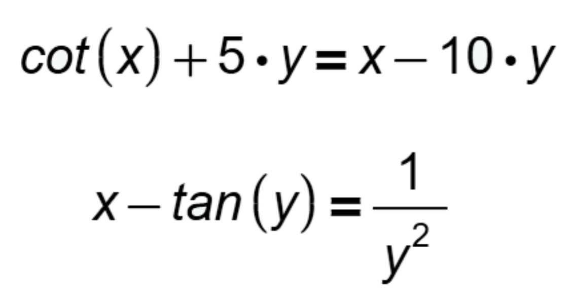
Consider as an educational process an applied lesson devoted to solving a system of two trigonometric equations, specifically chosen as:

$$\left\{\begin{array}{c}ctg\left(x\right)+5y=x-10y,\\ x-tg\left(y\right)=\frac{1}{y^2}.\end{array}\right.$$

(1)

The solution will be carried out using the popular mathematical package Mathcad (hereinafter, the version of Mathcad Prime 6.0 is used, unless otherwise stated). The entry on the Mathcad worksheet of the system (1) differs little from the usual mathematical notation (Figure 1):

It is advisable to first analyze the system of equations with the students, indicating its domain of definition $\left(x\ne \pi k;y\ne 0, y\ne \frac{\pi }{2}+\pi k, k=0,\pm 1,\pm 2\dots \right)$ and noting that due to the periodicity of the functions included in the system, the number of solutions will be infinite.

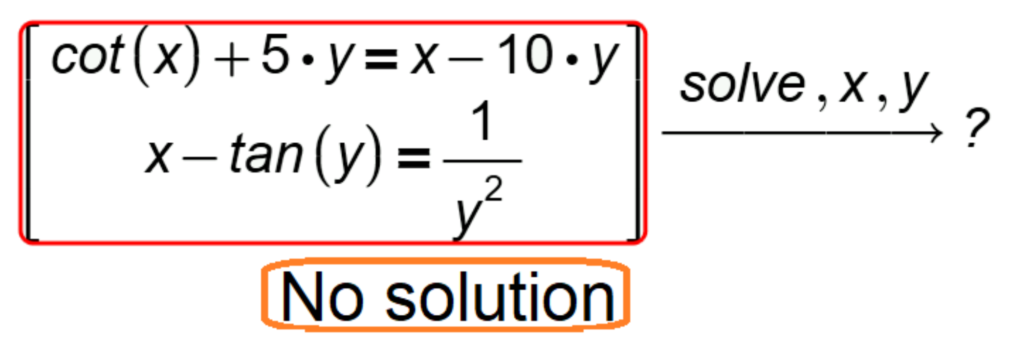
Further, it should be noted the possibility of solving equations and their systems using computer packages in three ways (symbolic, numerical and graphical) and indicate that the symbolic method is preferable, which gives all the exact roots of the system of equations. Then, the teacher should offer the students an attempt to solve the system of Equation (1) in the Mathcad environment by calling the operator of symbolic mathematics solve. However, anticipating the disappointment of students, it should immediately be noted that in case of failure, the plan is to move on to solving by other methods (numerical and graphical).

The solution of the system of equations in the Mathcad environment through the call of the operator of symbolic mathematics solve was not found by the students (Figure 2). Here, it is appropriate for the teacher to note that this was the expected result, since it is difficult for a computer package to display an infinite number of roots.

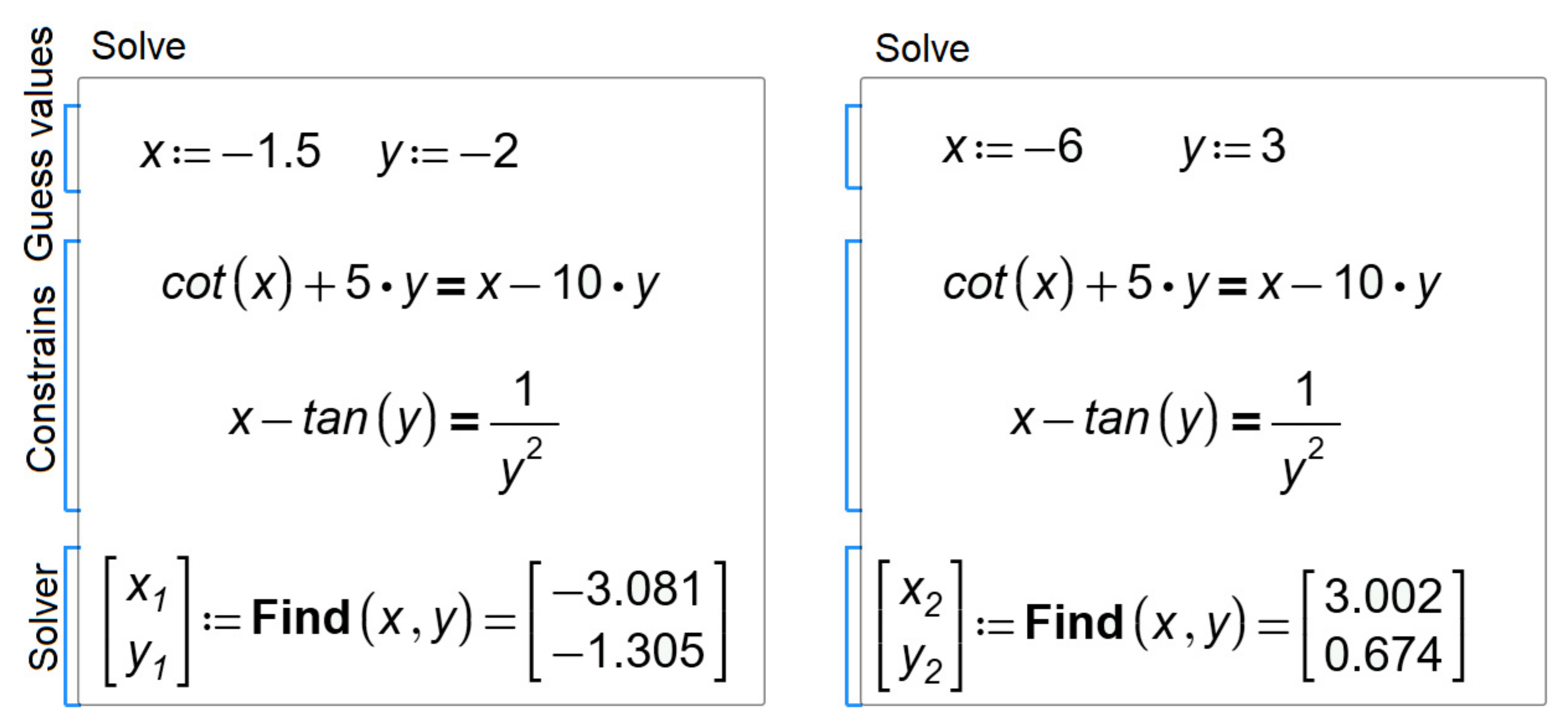
After that, as mentioned above, the teacher suggests moving on to a numerical (that is, approximate) solution of system (1), noting that this is quite satisfactory for most engineering calculations. Here, it is important to clarify that for the numerical solution, it is necessary to set the initial conditions as a given starting point for the calculation. The teacher should give students two pairs of initial conditions corresponding to the domain of the system (1) and offer to solve the system for two cases using the Solve numerical solution block (Figure 3).

After all the students are able to complete this assignment, the teacher needs to push them to an independent conclusion that the numerically found roots of the system depend on the choice of initial approximations. Then, the teacher can set aside some time for the students to experiment themselves, choosing various initial approximations at their discretion and getting more and more new roots of the system of equations.

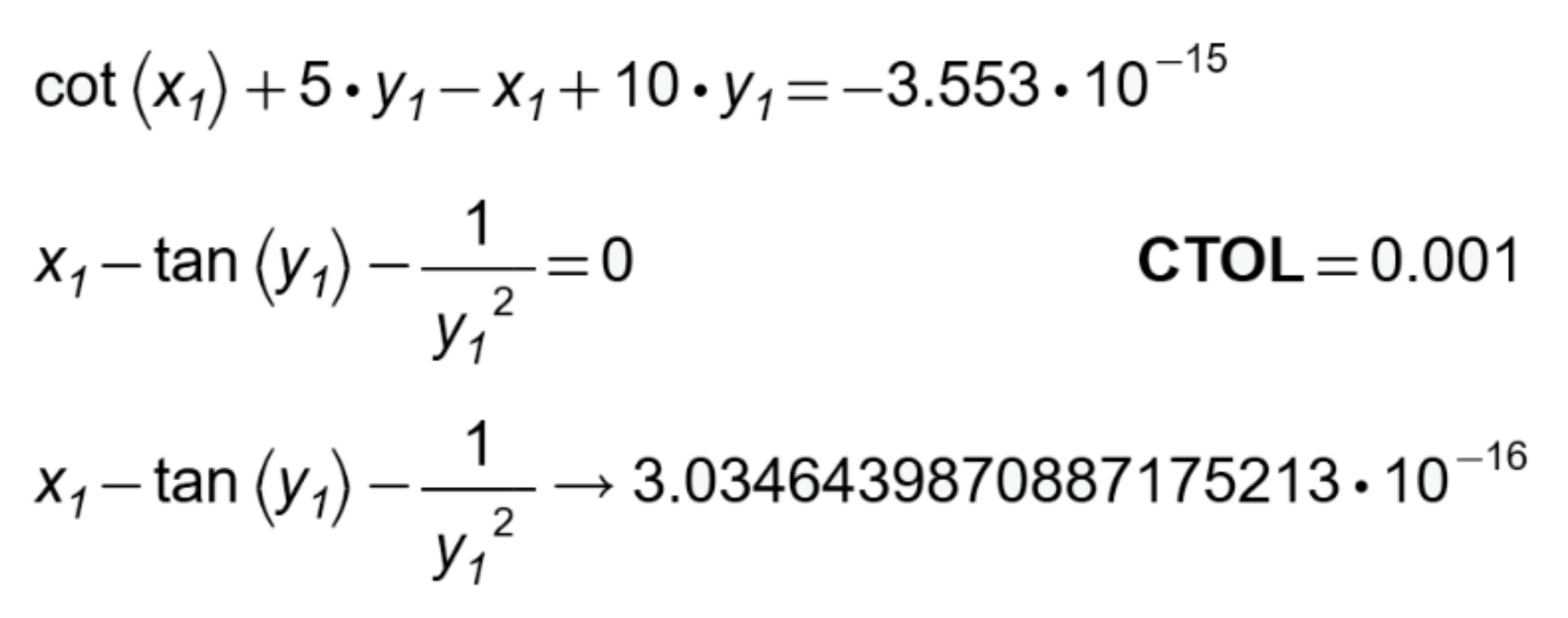
Note that the teacher does not delve into the question of what specific numerical method for solving equations is implemented in the used Find function. Now it is important to focus students’ attention on checking the correctness of the obtained numerical solution with the given accuracy CTOL (ConstrainsTOLerance) (Figure 4), which they must carry out independently by substituting the found roots into the equation and setting the required value of CTOL.

Upon completion of the numerical search stage of the solution to system (1), the teacher concludes that the solutions, in a large proportion, were found randomly, and a clear picture of the location of the roots is not yet formed. Therefore, it is necessary to move on to the third graphical method of solving system (1), using Mathcad visualization tools. Since at the initial stage of learning, plotting in Mathcad is inevitably associated with many small syntactic errors, the search and correction of which will take a lot of time for students and distract them from the main goal of the lesson, it is first advisable to use the online resource WolframAlpha [36], where plotting is extremely simple (Figure 5). The resulting plot (Figure 5) serves the purpose of initial visualization very well, giving an idea of the infinite number and arrangement of roots. It is necessary to make sure that all students understand the meaning of the resulting image: the Cartesian plot shows curves that display individual equations and their intersection points are the roots of the system (1).

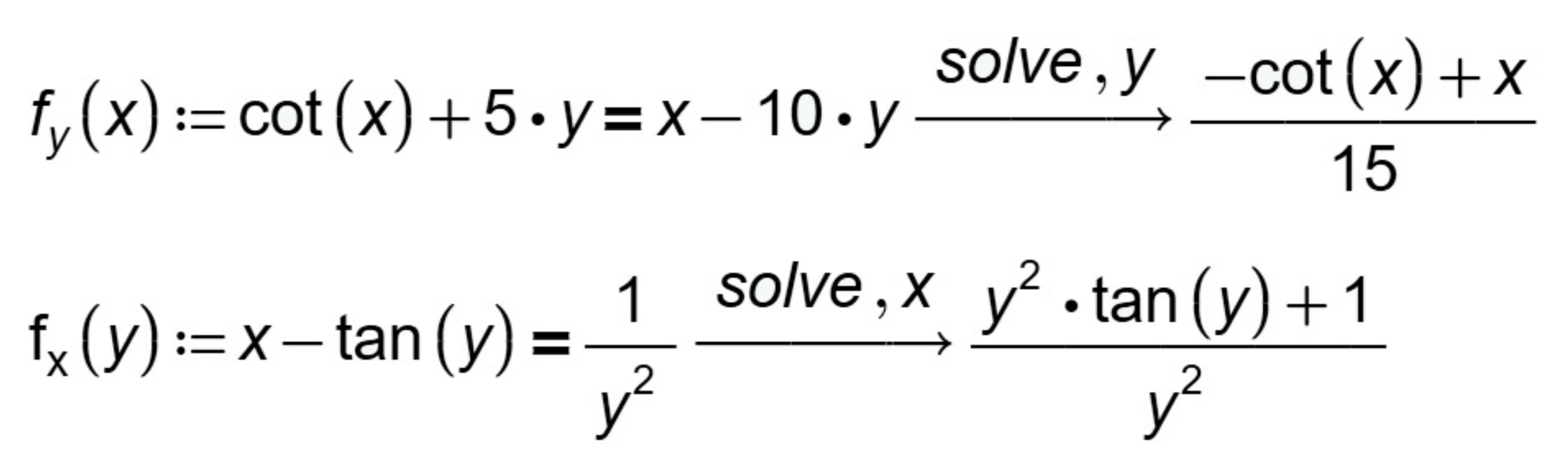
Now it is possible to proceed with the construction of similar graphs in Mathcad. To do this, it is necessary to first resolve each equation of system (1) with respect to one variable (one that is not an argument of the trigonometric function) (Figure 6).

Then, the students need to build graphs of the obtained functions, arranging the arguments and functions on the axes in the particular way indicated by the teacher.

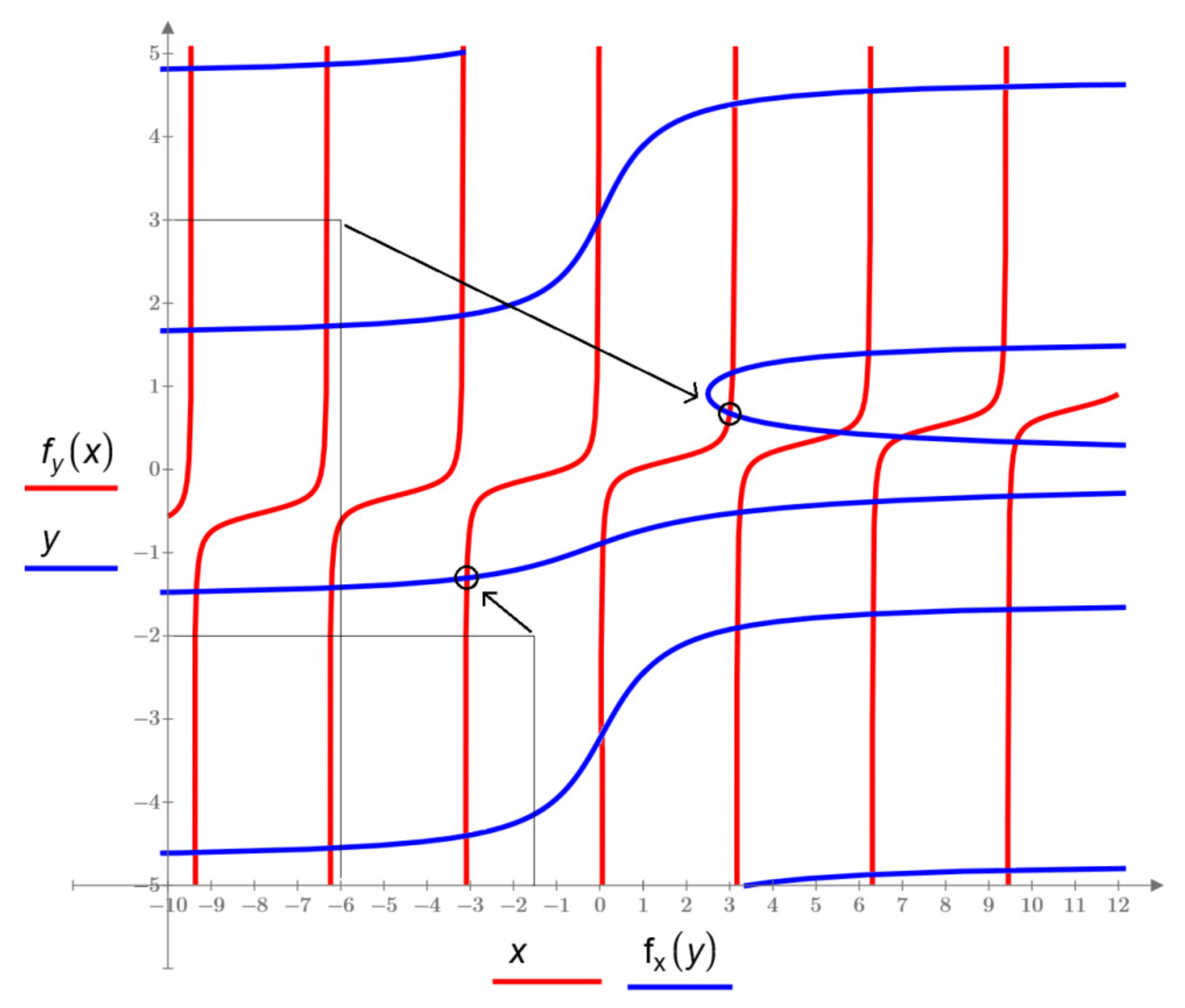
The visualization presented in Figure 7 gives a much more visual representation of the roots of system (1) than the graphs built in the WolframAlpha system. At the same time, the cognitive and motivational effect associated with the fact that students were able to understand the Mathcad graphical tools and build this visualization on their own is much higher.

Now that, thanks to the solution obtained with the described three methods, students have received a fairly complete and visual understanding of the roots of the system (1), the teacher can move on to more subtle questions about finding roots. To do this, you can, for example, analyze, using the constructed graph, how the chosen initial approximations and the corresponding roots are related (Figure 7 shows two arrows, the beginning of which lies at the points of the initial approximation, and the end of which lies at the corresponding found roots). The teacher notes and indicates on the graph that one of the solutions $\left(x=-3.081, y=-1.305\right)$ is the nearest root to the point of its initial approximation $\left(x=-1.5, y=-2\right)$, which looks logical. The same cannot be said for the second solution $\left(x=3.002, y=0.674\right)$, which is much further from its initial approximation $\left(x=-6, y=3\right)$ than other roots. It is necessary to explain that this phenomen depends on the algorithm of the Find function and to indicate a way to overcome this situation.

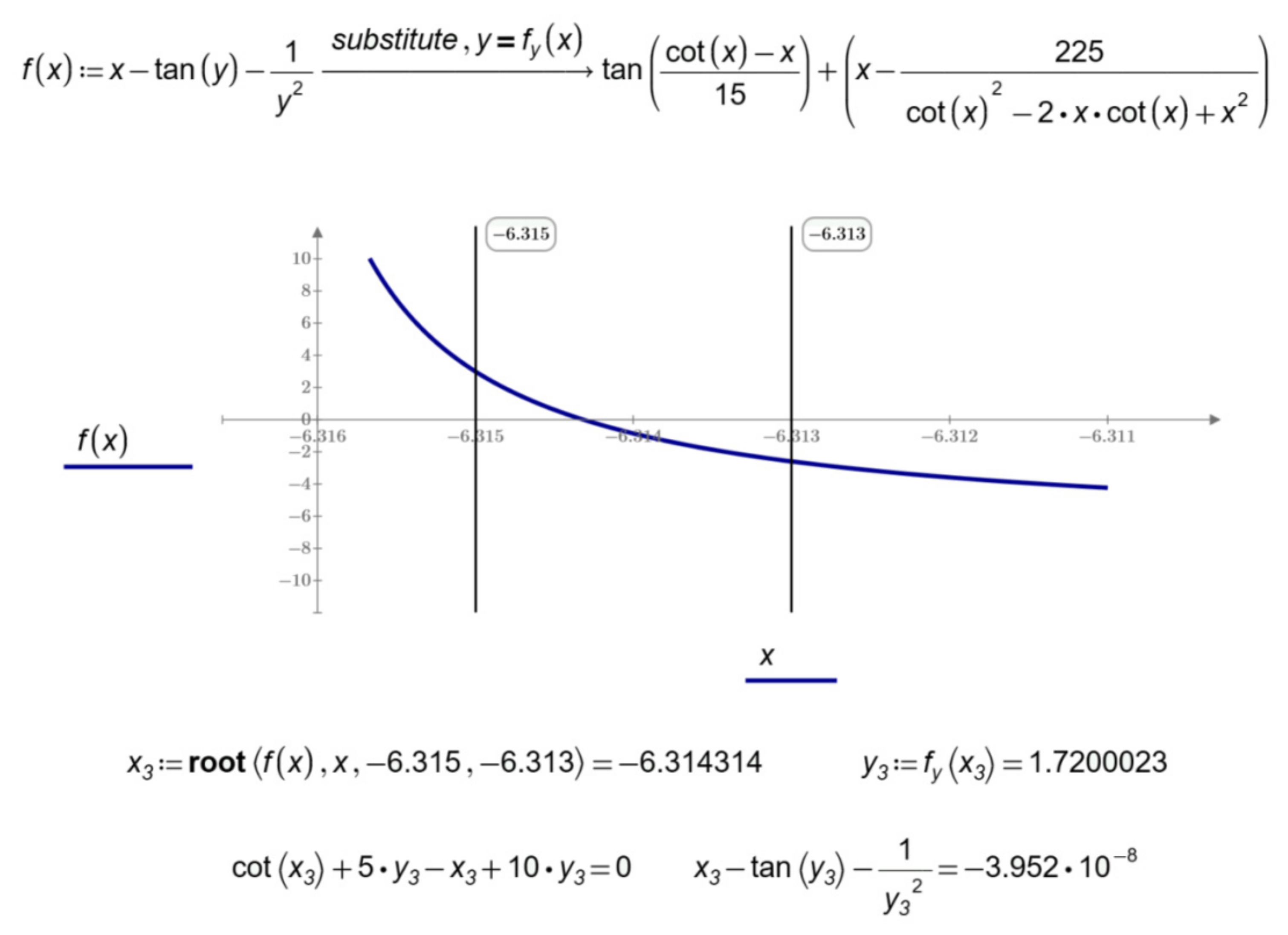
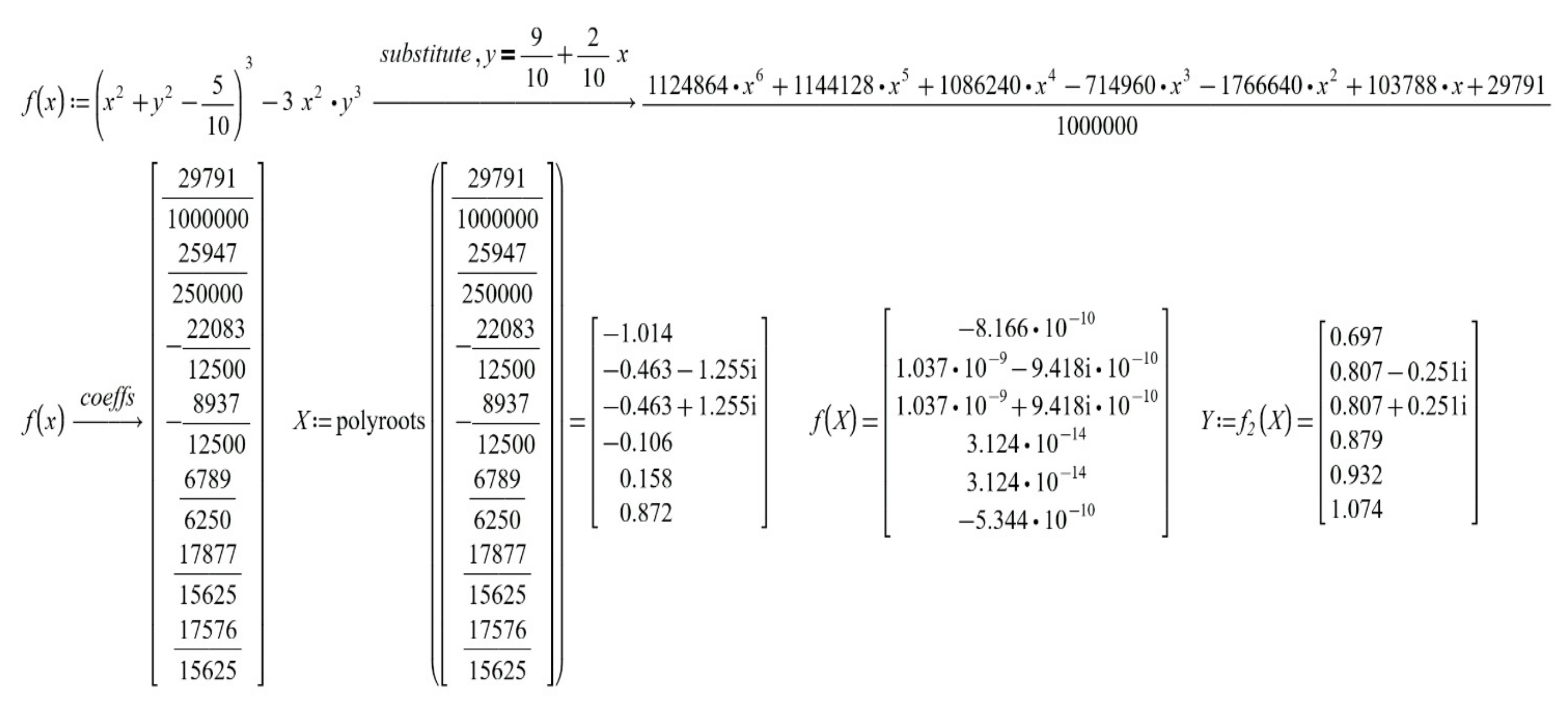
It should be clarified that in order to find the root closest to the initial approximation $\left(x=-6, y=3\right)$, it is possible, for example, to use another Mathcad tool—the root function. To do this, system (1) must first be reduced to one equation $f\left(x\right)=0$ with respect to the variable x by substituting the variable y expressed from another equation using the substitute operator (Figure 8).

Next, a graph $f\left(x\right)$ is built in the range of change of the variable x of interest to us (Figure 8). The teacher offers students visually, i.e., approximately determine the value of the root of the equation from the graph $f\left(x\right)=0$ (for this, it is possible to scale the axis of the graph in Mathcad). Then, the value of the root is found using the root built-in function with four arguments, two of which are the given values of the ends of the interval where the zero of the function is searched (Figure 8). Students should offer their own options for the end of the interval. After finding the root $\left(x=-6.31, y=1.72\right)$ (Figure 7) and its verification (Figure 8), it is necessary to make sure that all students can indicate the location of this root on the graph (Figure 7).

Summarizing the results obtained, it is important to note the obvious difference in using the Find function, which relies only on the initial approximation and the root function, which is based on the half division method and uses both ends of the interval.

Thus, using the example of solving a system of trigonometric equations, we outlined a practical lesson on mathematical modeling in the Mathcad environment. The effectiveness of the educational goals is achieved by students through their independent use of the various tools of the Mathcad package, visualization and the creation of situations of success.

3.2. Application of the Visualization Method by Creating a “Portrait” of the Numerical Search

In the previous section, an example of a learning process in a practical lesson was considered, which allowed students to fully develop the skill of independent work when mastering computer mathematical packages. In this section, we will consider the learning process using the example of a lecture session in which students will be more active listeners. For maximum involvement of students in a lecture session, it is necessary to take into account the emotional component [22,37], that is, the lesson should not only be informative, but also exciting, which is very effectively achieved with the help of visualization. This lesson continues and generalizes the topic of finding the roots of equations and their dependence on the initial approximation and should be carried out after the lesson described in the previous section, which plays the role of a stimulating example.

The lecture session can be conditionally divided into two parts: the use of the visualization method for the numerical search for the roots of a system of equations (first part) and for the numerical search for extremum points of a function of several variables (Second part).

3.2.1. Application of the Visualization Method by Creating a “Portrait” of the Numerical Search for the Roots of a System of Equations

In the first part of the lecture, it is proposed to consider a system of two equations:

$$\left\{\begin{array}{c}{\left(x^2+y^2-0.5\right)}^3=3x^2{y}^3,\\ y=0.9+0.2x.\end{array}\right.$$

(2)

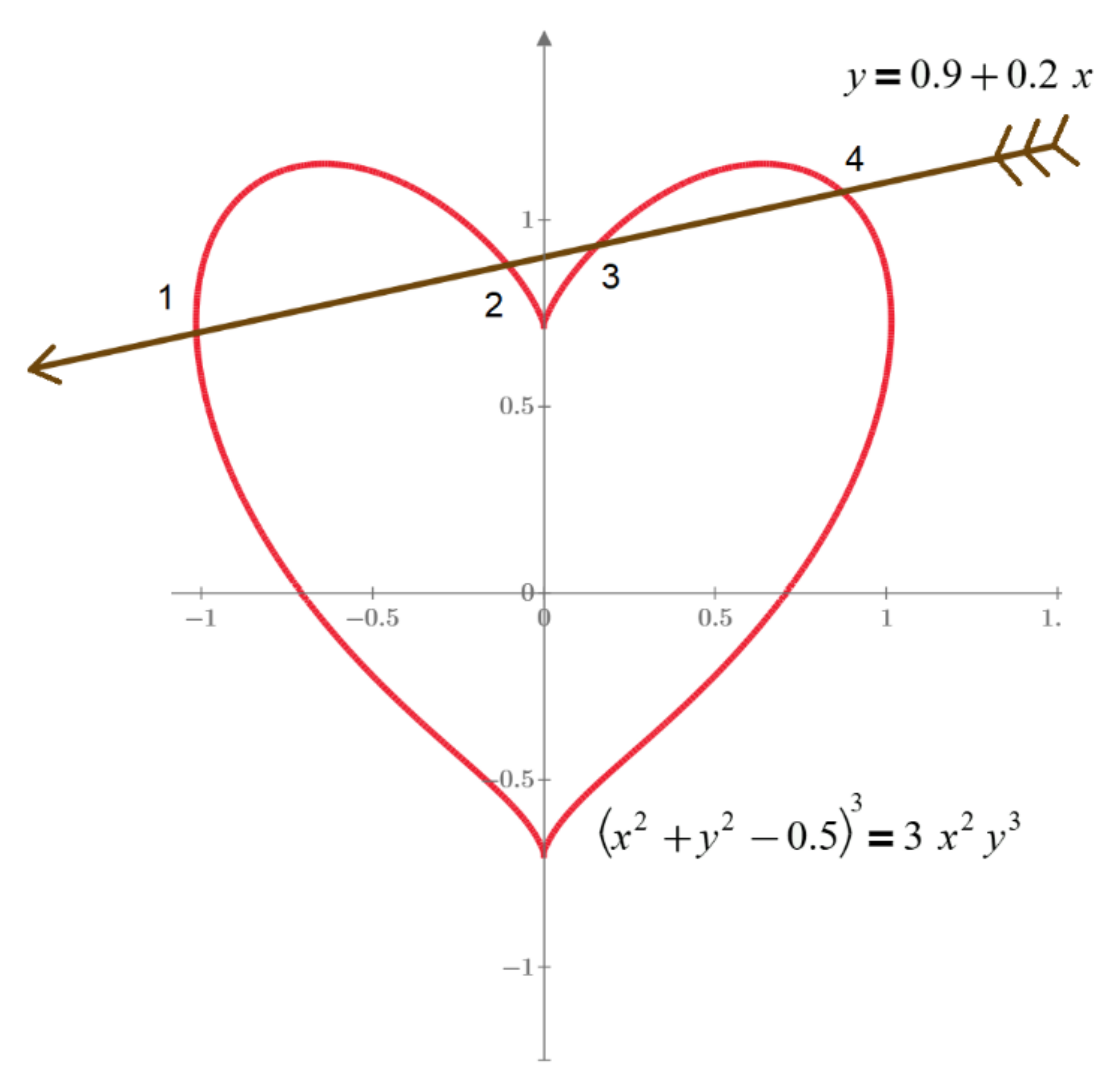
Students are immediately invited to familiarize themselves with the graphs of the polynomials included in (2), built in Mathcad (Figure 9).

The type of graphs will undoubtedly interest students, since it represents a “heart pierced by an arrow.” It should be explained to students that, strictly speaking, the graph of the second function is a straight line and the “arrow” is obtained by creatively refining the drawing. Having received the emotional response of students to the presented visualization, it is necessary to analyze the system of equations with the students: to note that the number of roots of system (2) is six and to discuss why only four of them are visible on the graph (system (2) has two more complex roots).

Students should be reminded of the conclusions that were drawn from the results of the previous lesson, where the system of the trigonometric Equation (1) was solved. Namely, it must be emphasized once again that the numerical determination of the roots of system (2), as well as system (1), will depend on the choice of the initial approximation. 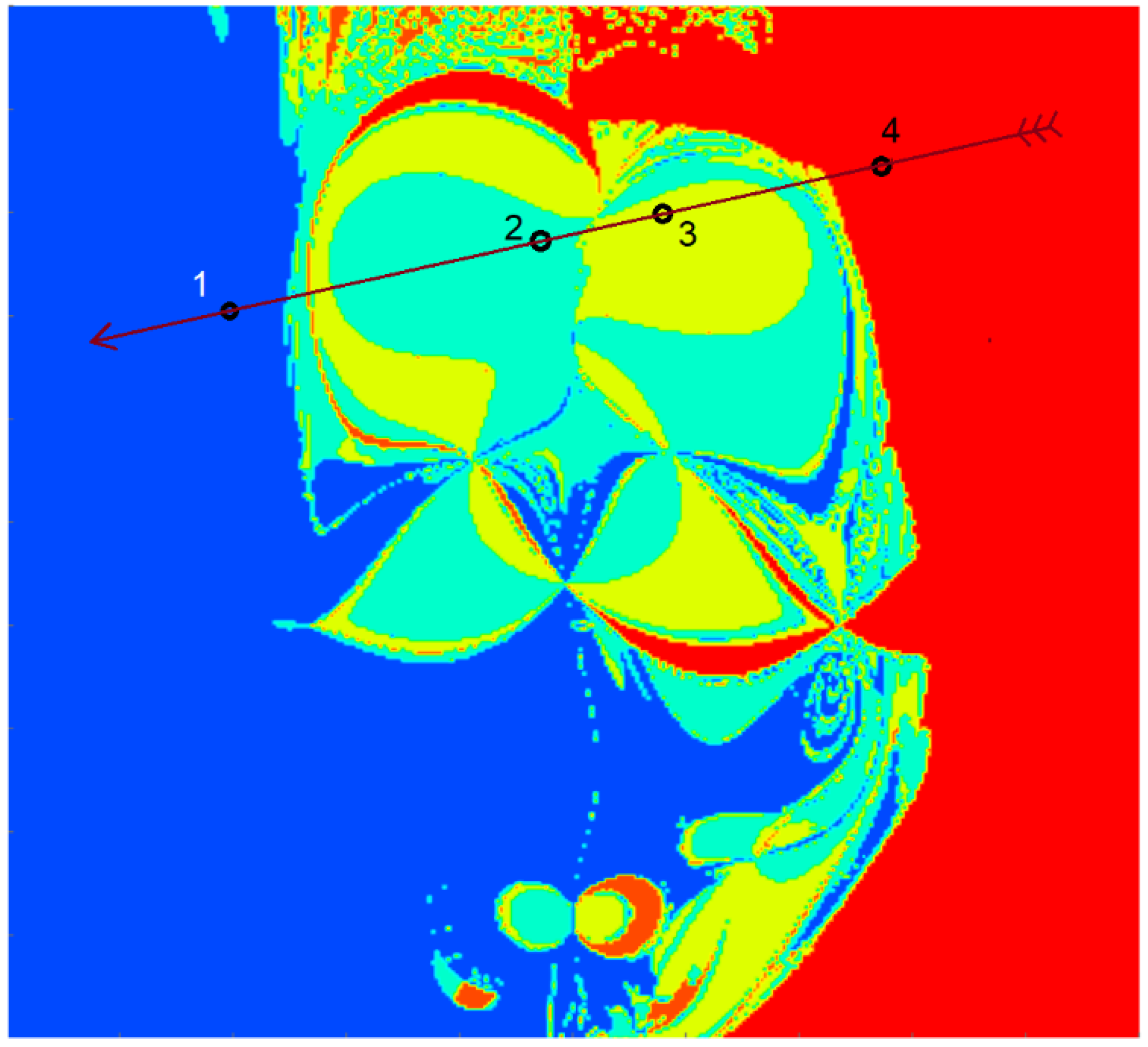That is, the selected valid initial approximation will lead to finding one of the four real roots shown in Figure 9. Which of the four? In order to answer this question, students are offered the following visualization prepared in advance by the teacher, which can be called a “portrait” of the roots of the system of Equation (2). This kind of visualization is used to evaluate numerical methods [32]. The visualization was obtained by scanning the area of the plane according to the graph in Figure 9. Four colors (blue, green, yellow and red) in Figure 10 designate the areas, by choosing the point of initial approximation in which we obtain the roots marked 1, 2, 3, or 4 as a numerical solution (2).

The visualization presented in Figure 10 once again clearly confirms the fact noted in the previous lesson: the root of system (2), corresponding to the chosen initial approximation, is by no means always the closest to it. It should be noted here that the Levenberg–Marquardt numerical method was used to construct this “portrait” [34,35].

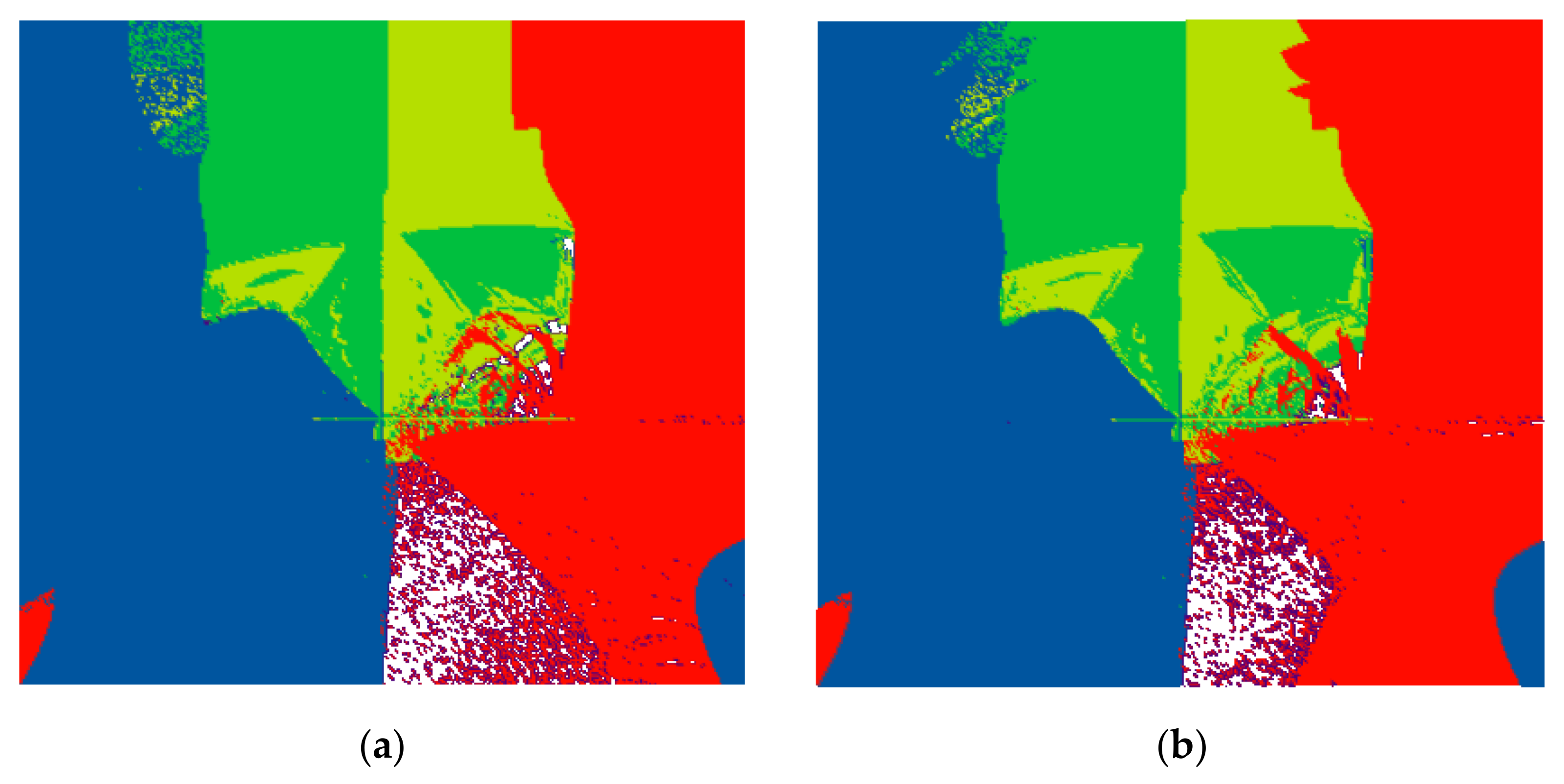
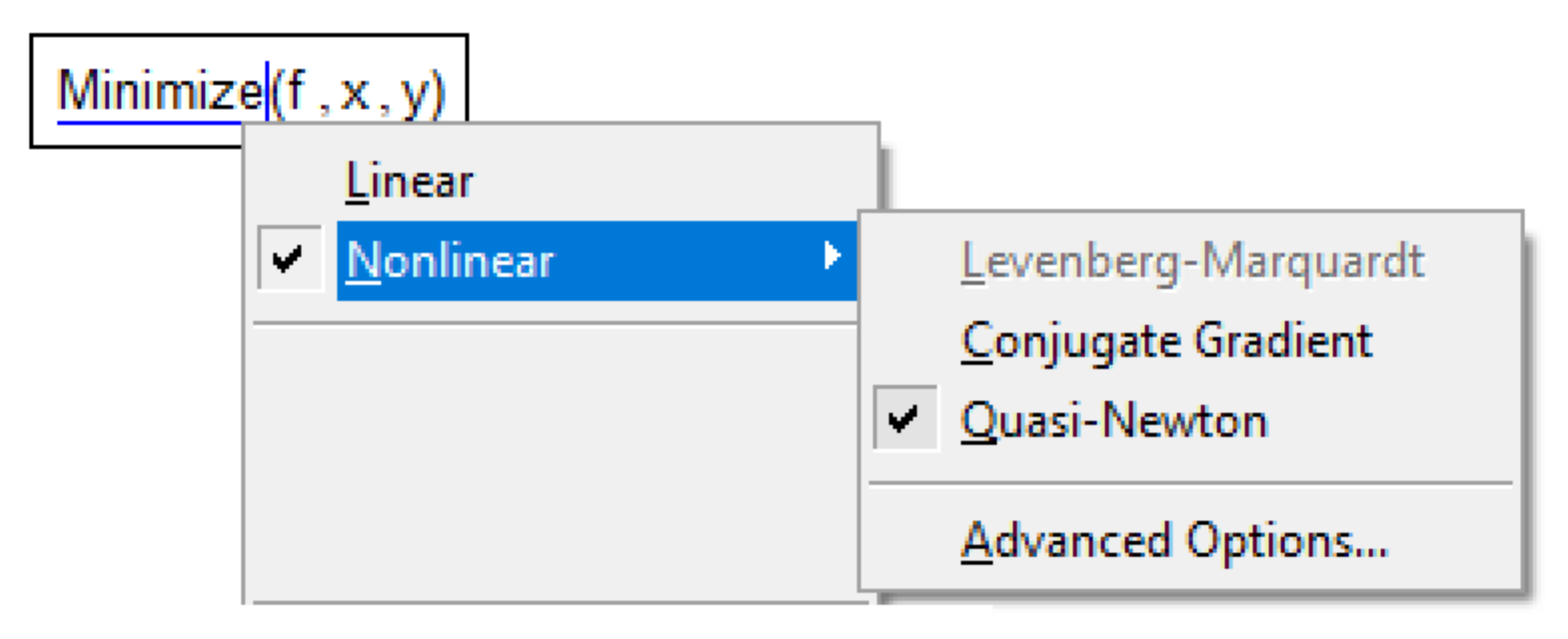
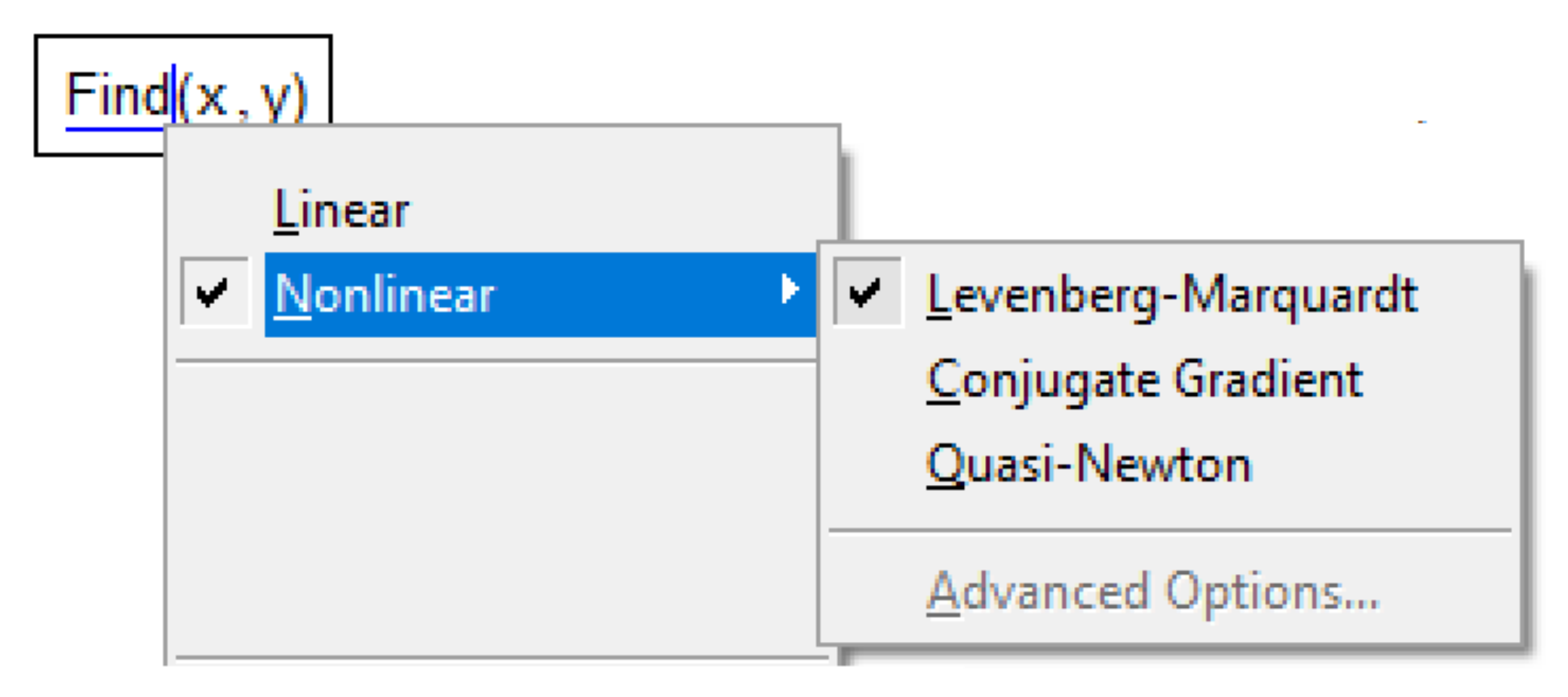
Is it possible to choose another method and will it give a better result? To answer this question, students are offered a visualization representing the portraits of the roots of system (2), obtained in the Mathcad 15 package using the Conjugate Gradient method [34,35] and the Quasi-Newton method [34] (Figure 11). Part of the program instructions in Mathcad 15, illustrating the tool for the selection of the numerical method, is shown in Figure 12.

It is easy to see that in Figure 11, areas of another (white) color appeared. The teacher should first invite students to express their hypotheses regarding the meaning of these areas (these are areas where the initial values are located in which the numerical solution was not found in Mathcad 15).

Then, students are invited to draw a conclusion about the effectiveness of various numerical methods in solving this problem based on a comparison of Figure 10 and Figure 11. In this case, the Levenberg–Marquardt method turned out to be more effective, which allows for the solving of system (2) for any initial value from the considered part of the plane. It is useful to note that for this reason, in the Mathcad Prime package, the developers left only the Levenberg–Marquardt method available for use, excluding the Conjugate Gradient method and the Quasi-Newton method.

When students have received a sufficiently complete idea of the assignment as a result to the visualizations (Figure 9, Figure 10, Figure 11 and Figure 12), the teacher can proceed to search for the roots of the system (2) by reducing it to one equation $f\left(x\right)=0$ with respect to $x$. 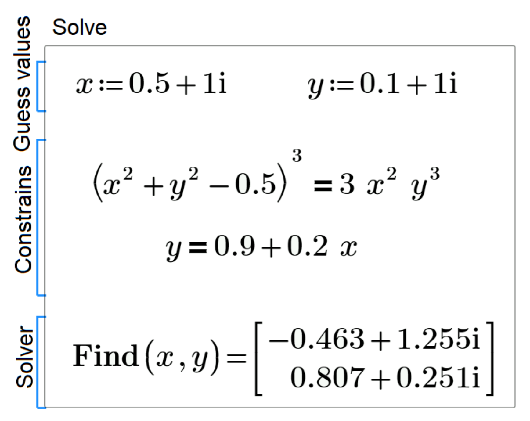The teacher reminds that, as in the case of system (1), this operation is carried out in Mathcad using the substitute operator (Figure 13). It is important to draw students’ attention to the fact that system (2), unlike system (1), has a finite number of roots. Therefore, in this case, in order to solve the equation, it is possible to use the Mathcad polyroots function, which allows one to get all six roots at once, including two complex ones. With the help of Figure 13, the teacher analyzes the syntax of the polyroot function with students and demonstrates the result of the solution and its verification.

To consolidate the studied material, it is useful to suggest students, as independent work in the subsequent laboratory lesson, find the real roots of system (2) using the Solve numerical solution block (as was done earlier for system (1)), choosing initial approximations according to Figure 10 and Figure 11. It is also necessary to draw students’ attention to the fact that one can find the complex roots of system (2) in the same way by choosing complex initial approximations (Figure 14).

To consolidate the emotional effect of the topic discussed, the teacher moves on to the most fascinating form of visualization—animation (https://community.ptc.com/t5/PTC-Mathcad/Portrait-of-roots-of-two-equations/m-p/776602, accessed on 20 July 2022). An animation based on Figure 9 is considered, where a straight “arrow” moves from bottom to top parallel to the Ox axis. Figure 15 shows several frames from the proposed animation.

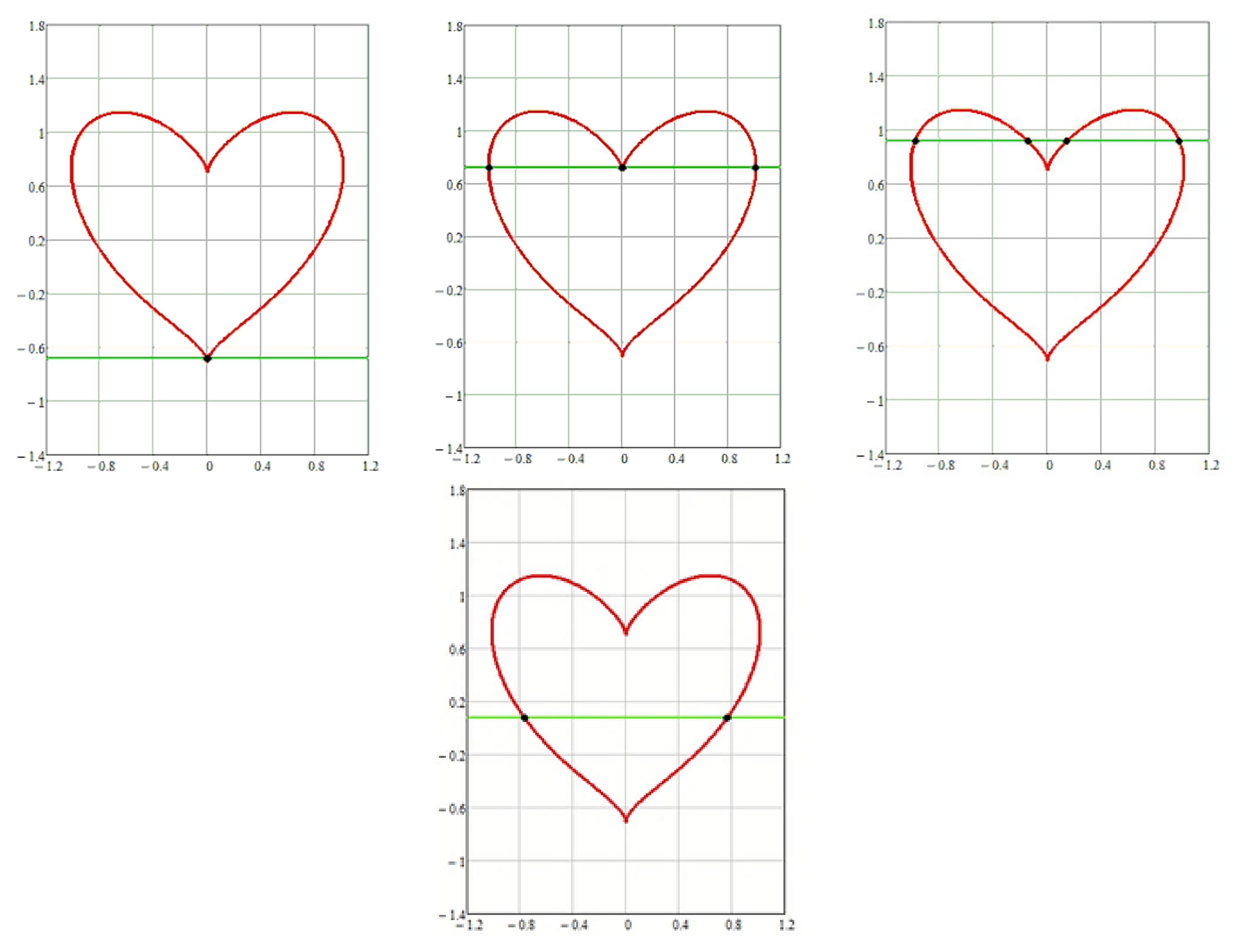
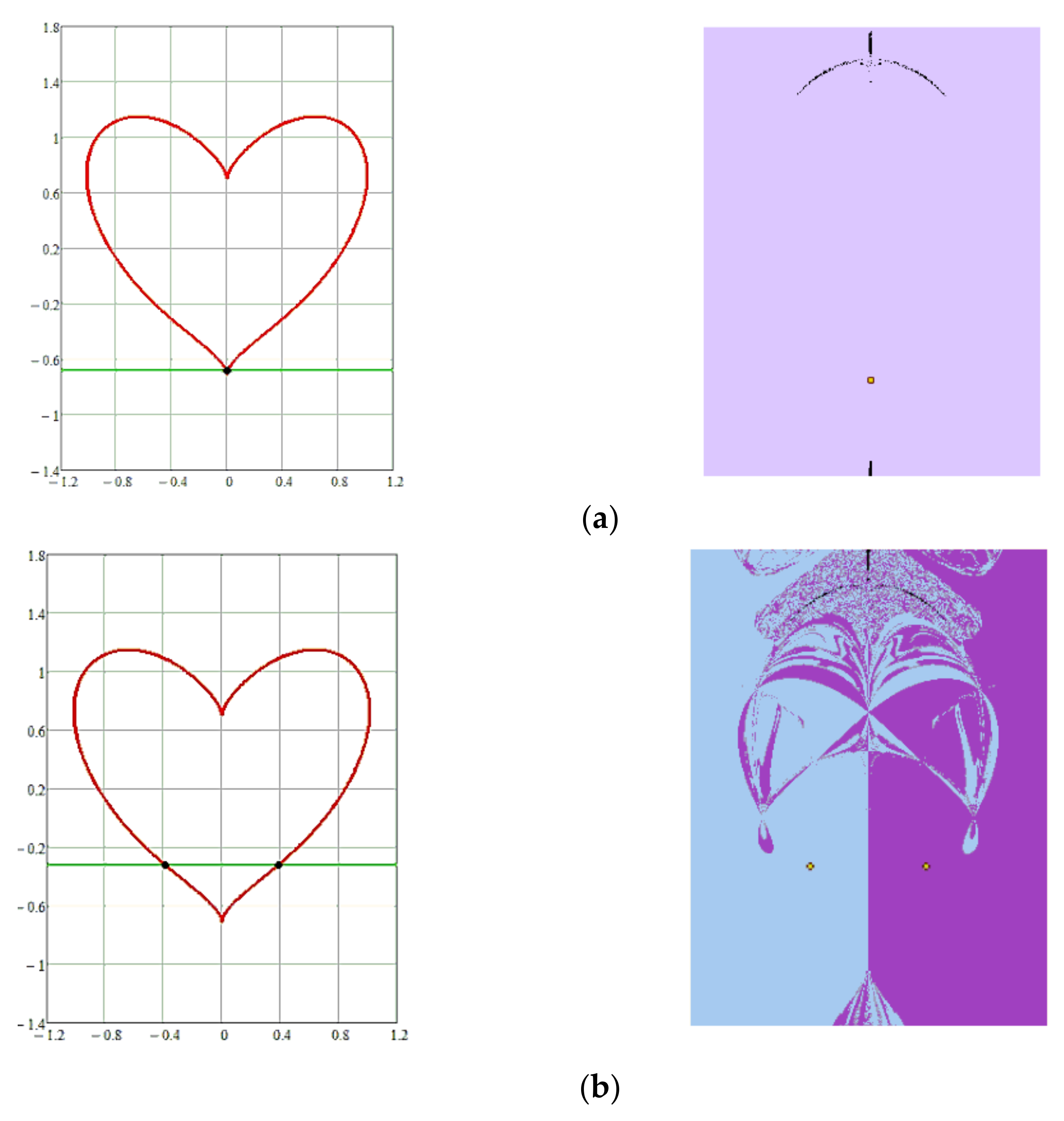
It is recommended to discuss with students what the system of Equation (3) looks like for each of the positions of the line:

$$\left\{\begin{array}{c}{\left(x^2+y^2-0.5\right)}^3=3x^2{y}^3,\\ y=a,\end{array}\right.$$

(3)

where a is a real parameter that changes during the animation.

It should be noted how the number of real roots of the system changes when the straight line moves $y=a$ (from one to four); students should also be invited to give an example of the value of a, in which system (3) will not have real roots.

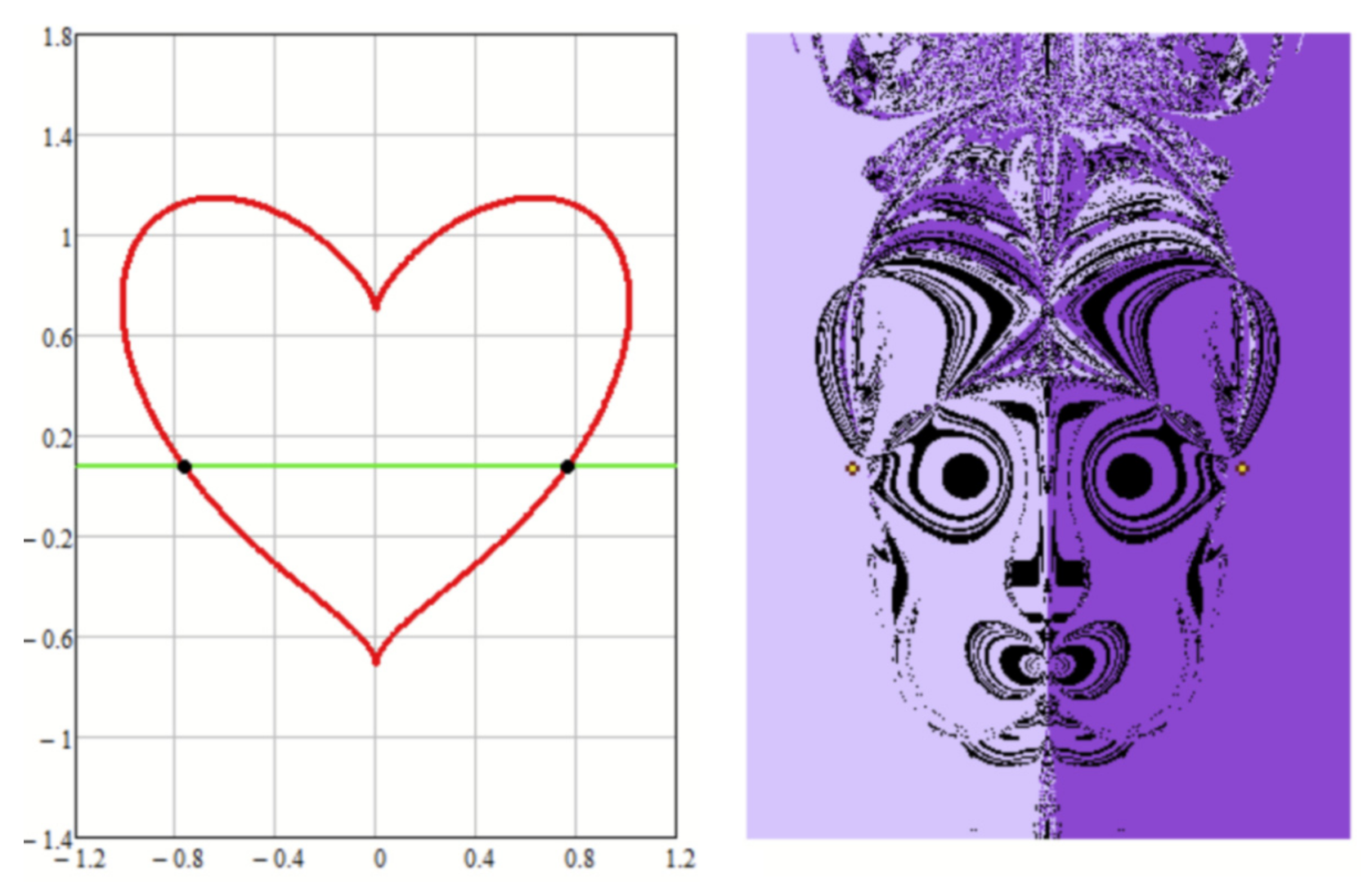
Next, students are invited to consider visualizations, which are “portraits” of the roots of the system of Equation (3) for different positions of the straight line, obtained by the Levenberg–Marquardt method in Mathcad 15 (Figure 16). Figure 16 shows visualizations for the case of one, two and four real roots. The most impressive is the visualization presented in Figure 17 for the case y = 0.082, where the “portrait” of the roots becomes a “sinister portrait” in the literal sense.

Continuing to reveal the purpose of the lesson, it is necessary to pay attention to the number of color areas that make up the visualization. This corresponds to the number of real roots, not counting the black areas. If the last ones are chosen as an initial approximation, it is not possible to find a numerical solution using the Levenberg–Marquardt method.

3.2.2. Application of the Visualization Method by Creating a “Portrait” of the Numerical Search for Extremum Points of a Function of Several Variables

In the second part of the lecture, the considered problem of choosing initial approximations is generalized to the case of searching for the extrema of a function, which is widely in demand in mathematical modeling in engineering [38].

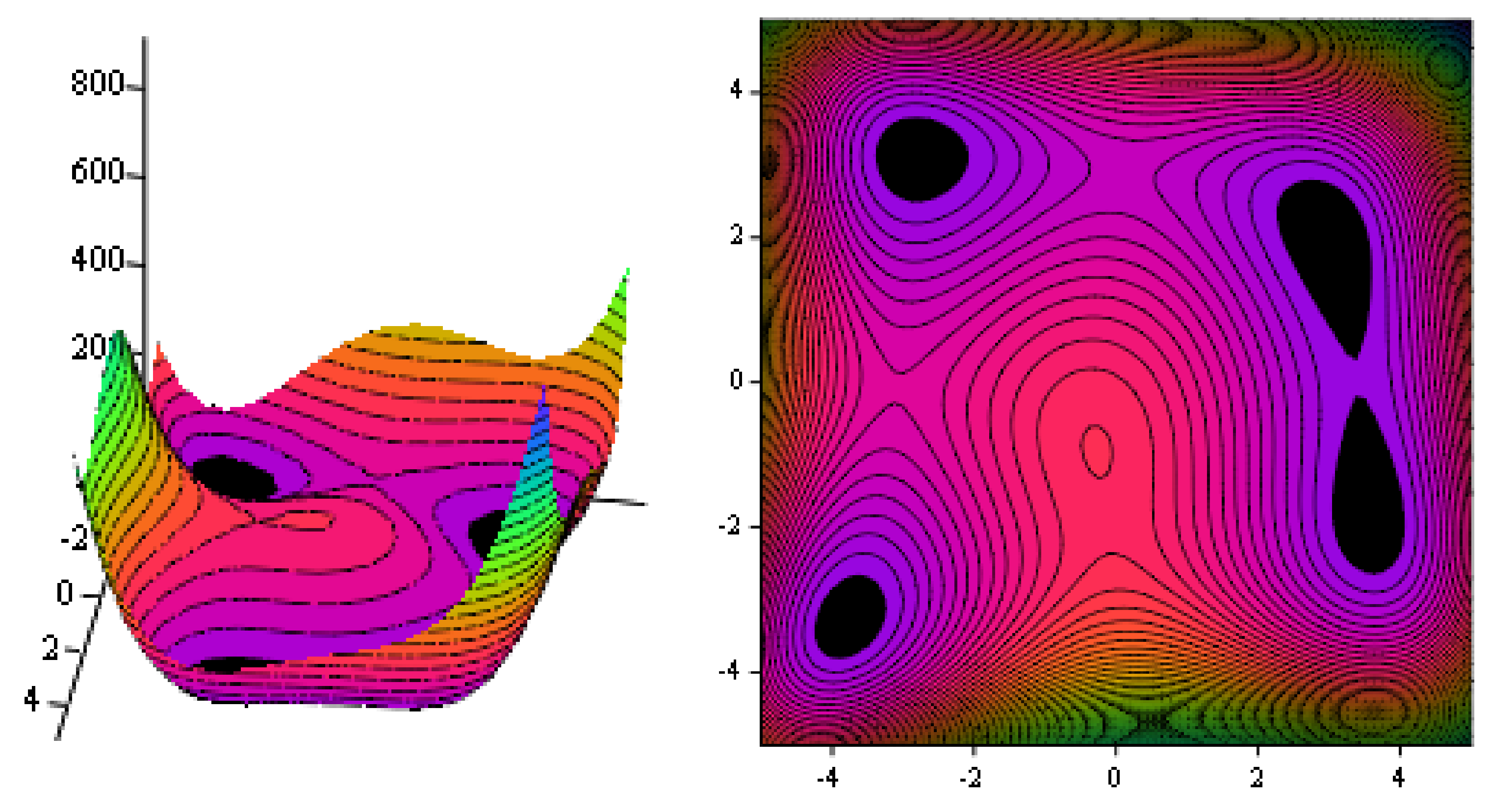
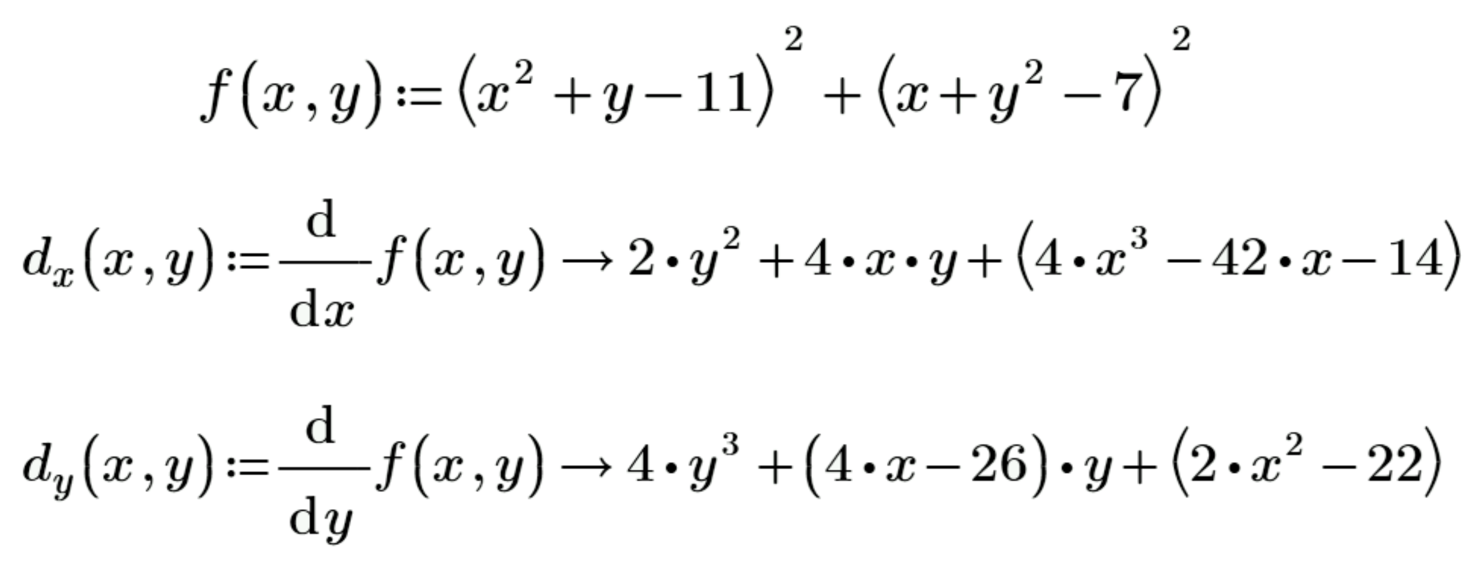
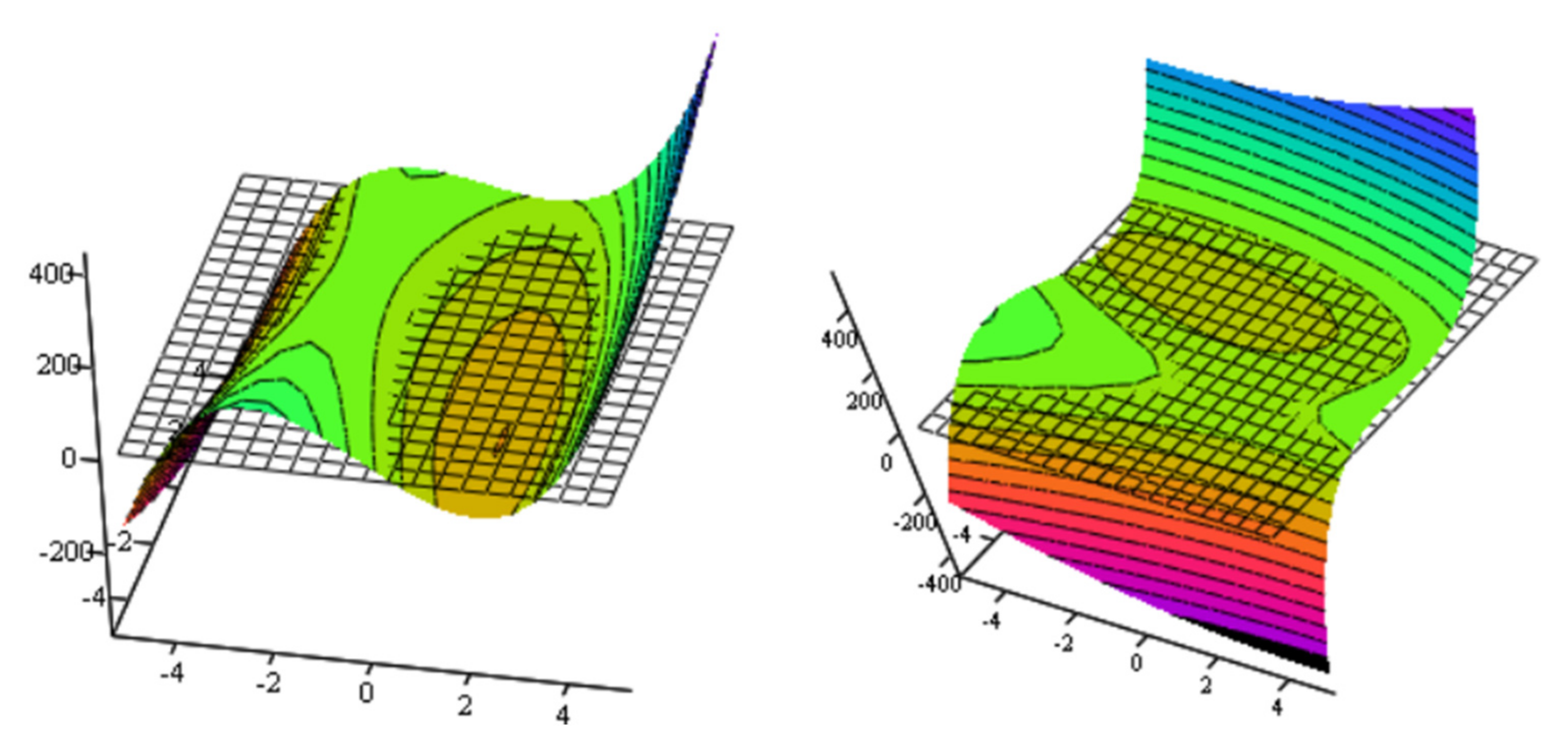
Students are invited to consider the Himmelblau’s function, which is used to test optimization programs [24,25]. The teacher shows the graph of the surface $\left(x,y\right)$ and the corresponding isolines, demonstrating the presence of five extrema in this function—one maximum and four minima, which are surrounded by lines of the same level (Figure 18).

After that, the teacher proceeds to consider various ways to search for extremum points using Mathcad tools.

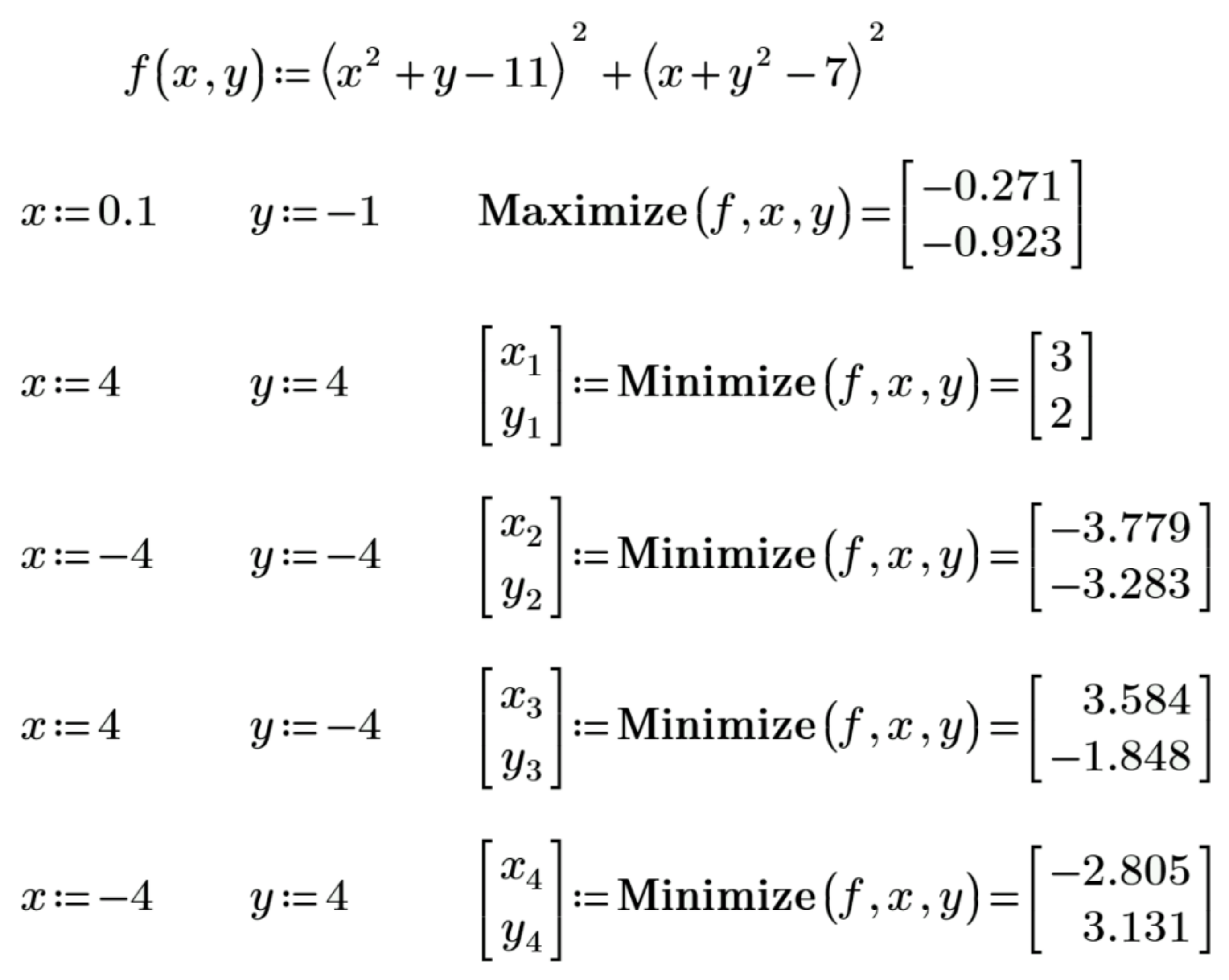
First, the teacher explains to the students that it is possible to find the maximum and minimum points of the Himmelblau’s function using the built-in Mathcad functions Maximize and Minimize, and in this case, it is also required to specify the initial approximations (Figure 19).

It should be clarified that since an education assignment is being considered and the values of the extremum points of the Himmelblau’s function are known, the initial approximations were selected based on this. Therefore, it is of interest to visualize the “portraits” of the numerical search for the extrema of the function, namely, the areas of initial approximations obtained by scanning. The teacher brings to the attention of the students the visualization (Figure 20, Figure 21 and Figure 22) of the numerical search for the minima of the Himmelblau’s function, similar to Figure 10, Figure 11 and Figure 12, which were constructed for the system of Equation (2) considered in the first part of the lecture.

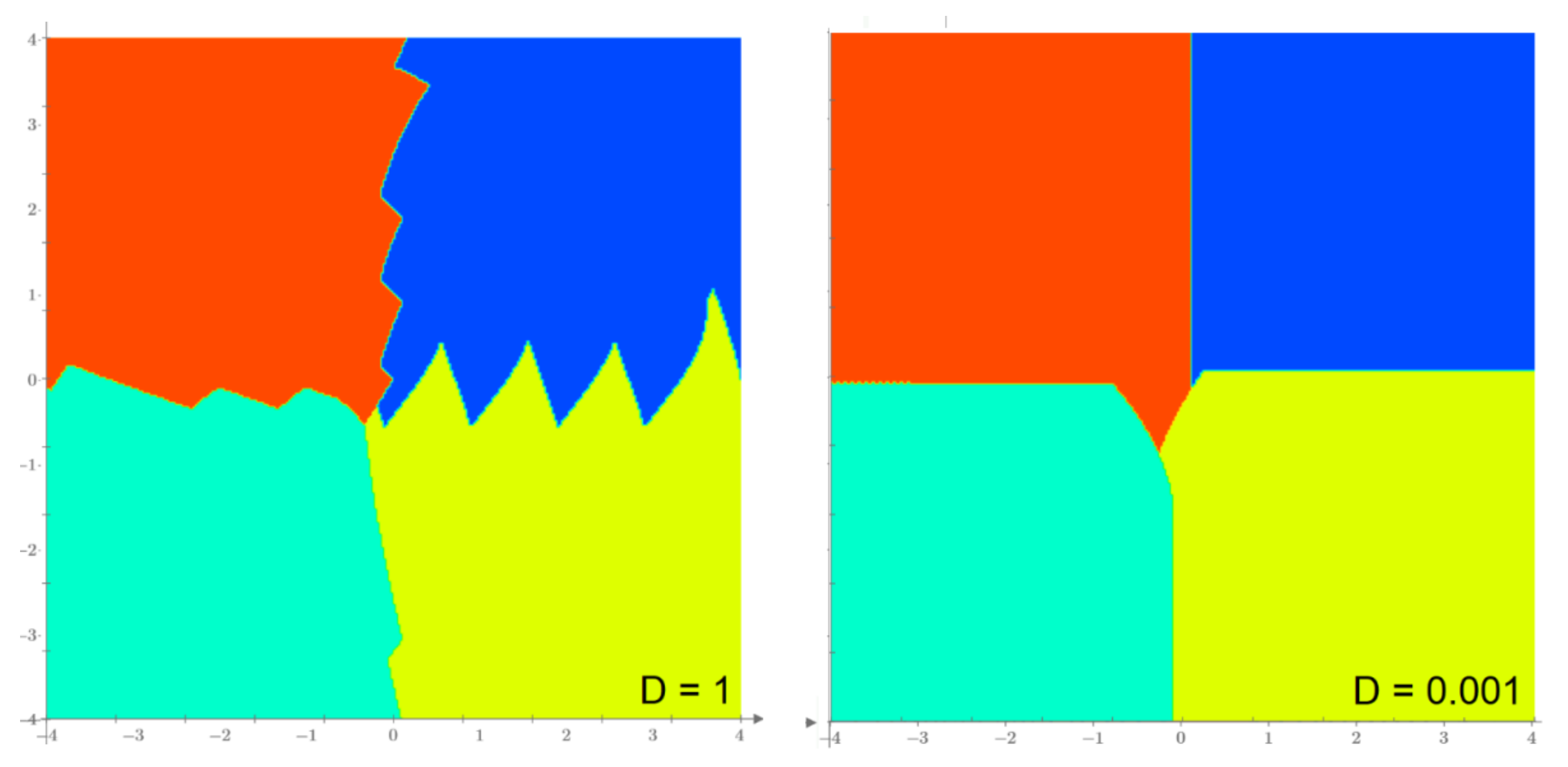
To consolidate the material, one should point out the similarities and differences between the visualizations in Figure 10, Figure 11 and Figure 12 with visualizations in Figure 20, Figure 21 and Figure 22 and ask students to make a conclusion about the comparative effectiveness of numerical methods for this case. Further, the teacher explains that in Mathcad it is possible to create a program that implements a custom numerical method using programming tools. An example of the code of such a program and the corresponding visualization of the regions of initial approximations for different steps D are shown in Figure 23 and Figure 24.

Students should focus on how reducing the D step of the custom numerical method affects the resulting visualization.

Then, the teacher proceeds to consider a second approach for finding extremum points, namely, the use of their mathematical definition. It is necessary to remind students that a necessary condition for finding the extremum points of a smooth function of two variables is the equality to zero of both first partial derivatives at these points (Figure 25).

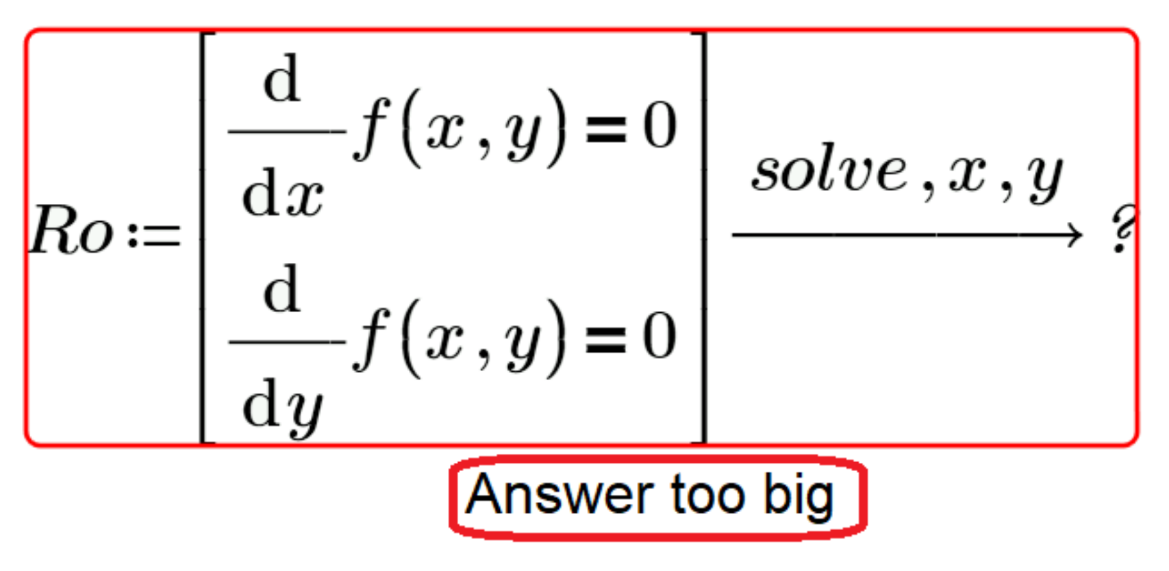
Figure 26 shows the use of symbolic mathematics—the solve operator—to find the roots of a system of two equations composed of partial derivatives of the Himmelblau’s function. It is recommended to discuss with students the question of why the number of roots obtained is nine.

Here, it is necessary to draw students’ attention to the following fact, obtained empirically, which can be very useful when using Mathcad. On the right side of the first equation of the system (Figure 26), there is a zero with a decimal point. In the absence of this point, Mathcad gives an incorrect result with complex roots (in Mathcad 15) or a message that the result is too large to display (in Mathcad Prime, Figure 27).

From this fact, we can draw an important educational conclusion for students: using Mathcad for mathematical modeling, one cannot rely solely on the result of calculations in the package, but it is necessary to conduct a preliminary qualitative analysis of the problem and have a clear idea of what kind of results are expected to be obtained.

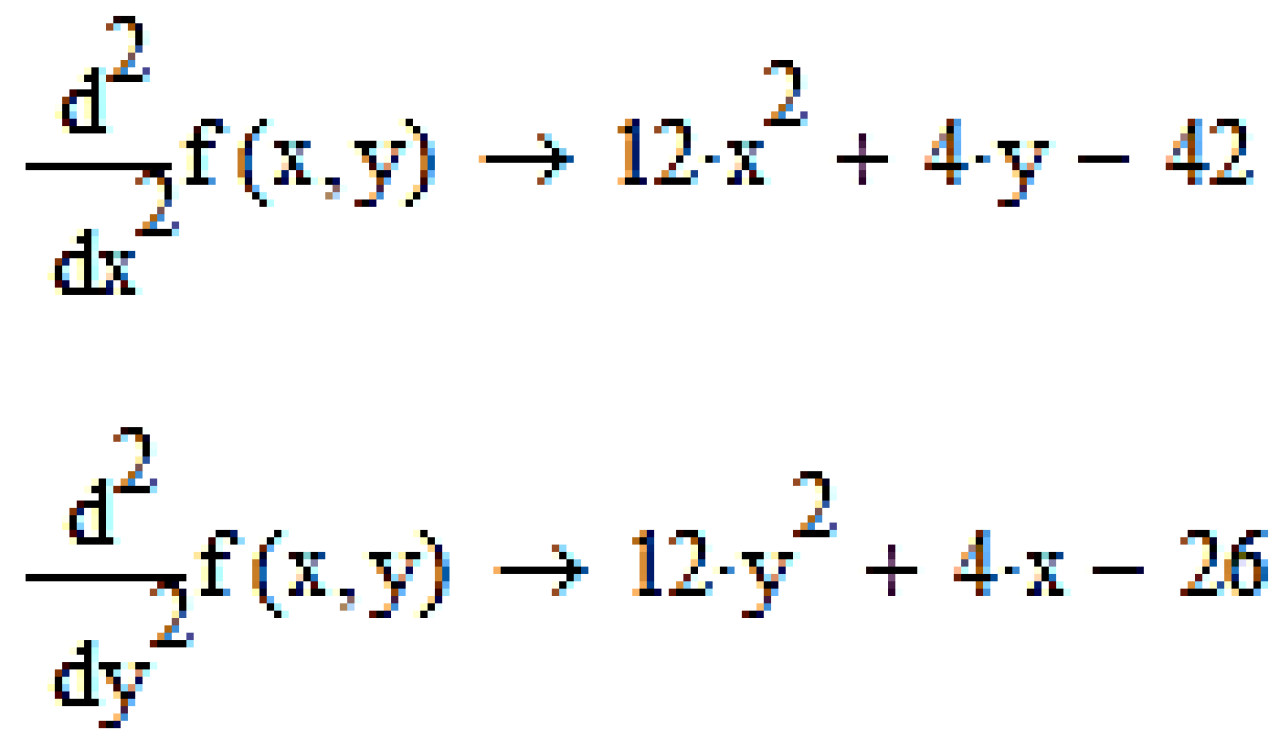
Finally, the teacher moves on to a third, graphical method of finding extrema. To do this, it is necessary to find the second partial derivatives of the Himmelblau’s function (Figure 28).

Students should be asked to compare the orders of the obtained first (Figure 25) and second (Figure 28) partial derivatives of the Himmelblau’s function. It is necessary to get the students to an answer to the question of which curves on the plane will represent the second partial derivatives. In addition, it is necessary to draw the attention of students to the fact that the graphs of the first partial derivatives are surfaces, therefore, only projections of lines of equal level to this surface can be built on a plane. In this case, we need projections on the Oxy plane of lines of equal level, on which the first partial derivatives are equal to zero. The teacher then presents views (Figure 29) showing the corresponding surfaces (graphs of the first partial derivatives) and the Oxy plane.

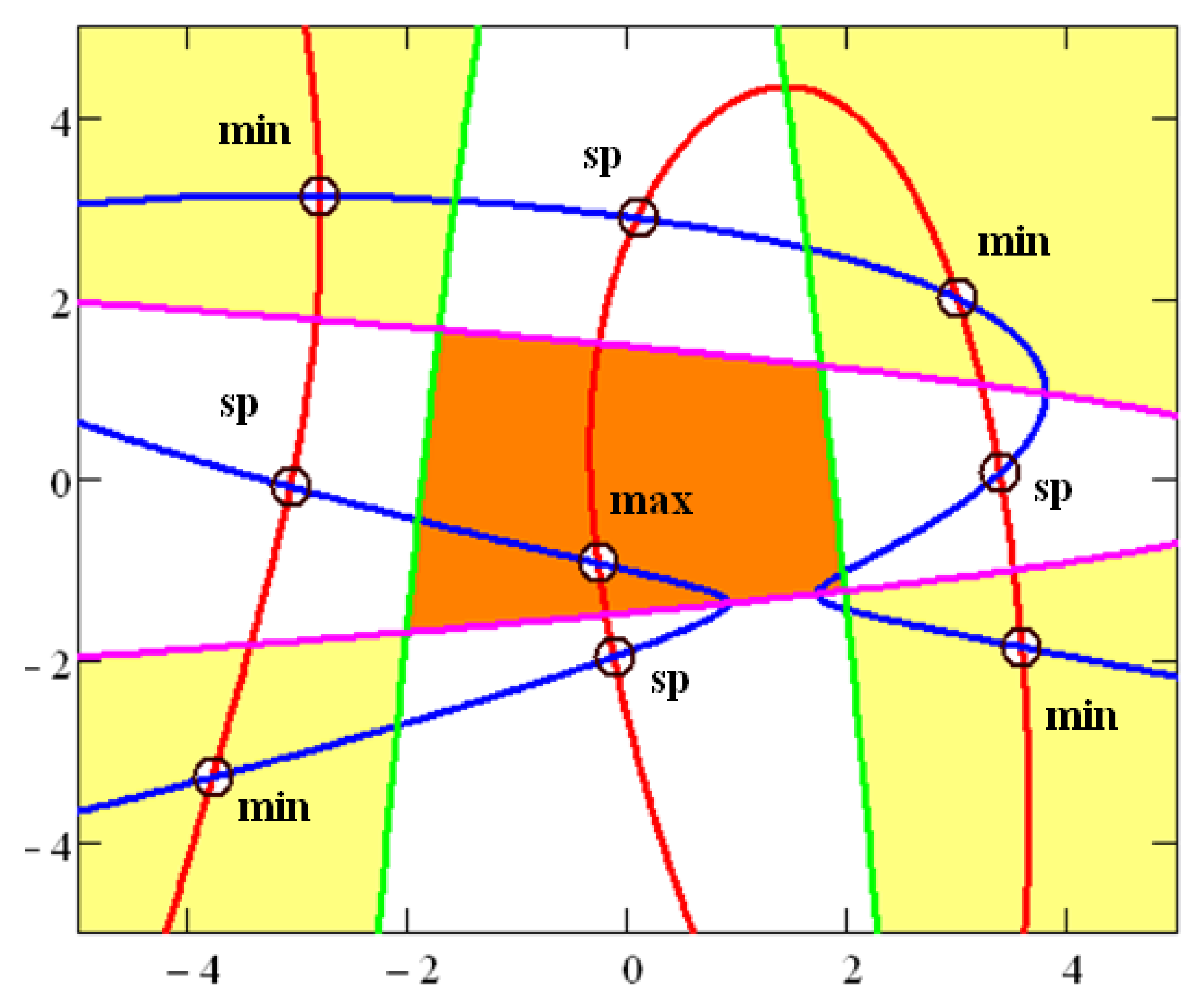
After that, the teacher suggests moving on to visualization (Figure 30), which shows the projections of the first partial derivatives of the Himmelblau’s function on the Oxy plane, as well as the second partial derivatives. Students are asked to determine which of the curves is which derivative (red curve is the first derivative with respect to x, blue is the first derivative with respect to y, green is the second derivative with respect to x, pink is the second derivative with respect to y). It is important to focus students’ attention on the relationship between the views shown in Figure 29 and Figure 30, which simplifies the understanding of the geometric meaning of the problem and further develops the students’ spatial imaging ability.

The visualization shown in Figure 30 allows students to visually demonstrate the necessary conditions for the existence of extrema and find them graphically.

Necessary condition: the critical points lie at the intersection of the first order partial derivatives with zero value (blue and red curves).

In addition, we should especially note the fact that nine regions of different filling around critical points are regions of guaranteed initial approximations for finding the roots of the system shown in Figure 26 using the numerical Conjugate Gradient method.

To consolidate the material studied, it is useful to offer students, as independent work in the subsequent laboratory lesson, to find extrema, as shown in Figure 19, choosing initial approximations in accordance with Figure 29 and using the Conjugate Gradient method (Figure 22).

Thus, in this section, we outlined a lecture using visualization in the Mathcad environment. We emphasized that as a result of visualization, students got a visual representation of the different numerical methods used in Mathcad packages and were able to conduct their comparative assessment. At the same time, it was possible to avoid a separate detailed description of each of the methods, which complicated the lecture session. Students achieved a complete understanding of the problem of finding the roots of an equation and choosing an initial approximation, as well as finding extrema of a function of several variables. Various possibilities of the Mathcad package were demonstrated. To consolidate the material, students were offered tasks for independent work. The effectiveness of the lesson and the achievement of educational goals were determined by the use of visual demonstration techniques, feedback from students, encouragement of independent conclusions, emphasis on the most significant issues, consolidation of previous material and an increase in the emotional background that arises from fascinating visualization.

3.3. Results of Acceptance of the Proposed Method

The proposed approach is an integral part of the experimental program carried out in the last few decades at the Department of Theoretical Bases of Heat Engineering of National Research University Moscow Power Engineering Institute. Within the framework of the educational discipline, “Information Technologies”, problems of systems of algebraic equations (for example, using the laws of conservation of energies and masses, balances of forces, etc.) that were sufficiently complex that they could not be solved analytically, were solved. Previously, they had to be simplified, which led to the loss of physical meaning. Students had to memorize or reproduce complex formulas for calculations from textbooks. The use of information technology, in terms of computer mathematical packages, such as Mathcad, MATLAB and Mathematica, made it possible to adopt numerical methods for solving equations, which enhanced the students’ understanding of the physical meaning of the equations and increased their confidence in their abilities and knowledge.

As noted earlier, numerical methods for solving equations have their own problems; in particular, issues associated with the choice of a first approximation. A poor choice of such an approximation often leads to failure in solving the problem. The proposed method of visual analysis of these areas of initial approximation has educational value in the sense that students have ceased to treat the computer as a kind of black box where they simply enter the initial data and extract the finished answer. As a result, classes have become much more entertaining and productive [39].

An analysis of class attendance and effectiveness showed that academic performance in study groups switched to learning technology, with computer visualization (flat and three-dimensional graphics, animation, etc.), increased by about 27% compared to study groups where classes were conducted with traditional technology [40]. This confirms the educational effectiveness of the proposed approach.

4. Conclusions

A method has been obtained for the use of visualization in computer mathematical packages, which makes it possible to clarify the difficult computational situations that arise for students when mastering these packages. Depending on the complexity of the problem being solved, either the teacher or the students themselves can create special visual graphic (animation) objects. Such objects allow, initially without going into the intricacies of the functioning of the package and the mathematical apparatus used, to competently describe a complete picture of a difficult situation for students and indicate ways to resolve it.

The method is considered through the example of the process of solving various systems of equations using the mathematical package Mathcad and the WolframAlpha online resource. Graphical and animated objects are presented that clearly demonstrate the areas of location of initial approximations and allow the student to numerically obtain all the real roots of systems of trigonometric and nonlinear equations.

Similar objects are constructed using this method for finding, as an example, the critical points of the Himmelblau’s special test function.

Visualization contents are confirmed by some presented computational calculations.

The method was tested during the training of university students at the National Research University Moscow Power Engineering Institute.

The proposed method can be applied in the broad context of the use of information technologies in mathematical and engineering education.