Numerical Simulation for Brinkman System with Varied Permeability Tensor ^†

Abstract

The aim of this paper is to study a stationary Brinkman problem in an anisotropic porous medium by using a mini-element method with a general boundary condition. One of the important aspects of the $P1-Bubble/P1$ method is satisfying the inf-sup condition, which allows us the existence and the uniqueness of the weak solution to our problem. To go further in this theoretical study, an a priori error estimate is established. To see the importance of this method in reality, we applied this method to a real problem. The numerical simulation studies support our results and demonstrate the effectiveness of this method.

1. Introduction

The purpose of this paper is to approach the Brinkman system using a finite-element method. The Brinkman system involves modifying the usual Darcy law by the addition of a standard viscosity term; this system was first defined by H.C. Brinkman [1]. In reality, many applications use this equation; for example, in a porous media it used to model fluid flow in a complex domain [2,3,4] and in a fictitious domain [5]. Shahnazari and al. worked on the nonlinear cases and products of the nonlinear Brinkman equation where the viscosity is nonlinear [6,7,8]. The Brinkman equations have very important practical applications in the field of anisotropic porous media [9,10,11], as well as in several other real domains such as nanofluids [12,13,14,15,16,17,18,19,20].

One important method for the resolution of differential equations is the mixed finite-element method (MFEM) [21,22,23]. This method has been used by several researchers to solve incompressible fluid flow problems [24,25,26,27]. Many research papers [24,28] are interested in solving the Brinkman equation using the mixed finite-element method, therefore the a priori and a posteriori error estimates for the Brinkman system are studied [28].

In this paper, we study the discretization, and we will establish the stability and a priori error estimate of the Brinkman problem with the permeability as a matrix by the finite-element method (mini-element); this method was introduced by Arnold, Brezzi and Fortin [29]. The method $P1/P1$ is not stable, so to overcome this obstacle we propose to use the $P1-Bubble/P1$. The basic idea for $P1-Bubble/P1$ is that the construction of the mini-element starts with standard finite-element spaces for velocity and pressure and then enriches the velocity space such that the discrete inf-sup condition is satisfied. This method leads to a relatively low number of degrees of freedom with a good approximate solution [29,30,31].

The numerical study of this linear problem is obtained in the matrix form of large size; indeed, we propose an efficient (preconditioned) Uzawa conjugate gradient method to accelerate the convergence of the numerical solution derived from the one used with $P2/P1$ (or $P1-iso-P2/P1$) [32,33]. To simulate the Brinkman equation in a heterogeneous reservoir, we modified the code suggested by J. Koko for the generalized Stokes problem [34], such that our model is based on the permeability as a matrix.

This paper is organized as follows: The governing equations and assumptions to conserve the existence and uniqueness of the solution are described in Section 2; Then a presentation of the mini-element method and the notations used in the approximation of our problem is performed in Section 3; The important theoretical results—the stability and a priori estimation—are proved in Section 4; Finally, to see the importance of this method, we propose several numerical experiments in Section 5 to prove that the convergence of our method is validated for an exact solution example.

2. Governing Equations

Let $\mathrm{\Omega }\subset {ℝ}^d$, $(d=2,3)$ be a bounded open set with a Lipschitz boundary $\mathrm{\Gamma }$. The Brinkman system is represented by the following equations

$$\left\{\begin{array}{lll}-\nabla ·(\tilde{\mu }\nabla u)+\nabla p+\mu {\mathrm{K}}^{-1}u=f& in& \mathrm{\Omega },\\ \nabla ·u=0& in& \mathrm{\Omega }.\end{array}\right.$$

(1)

The system in Equation (1) is completed by the boundary conditions on $\mathrm{\Gamma }$ given by

$$A^{-1}u+B\left(\tilde{\mu }\nabla u-pI\right)·n=g\hspace{1em}\hspace{1em}\mathrm{on}\hspace{1em}\mathrm{\Gamma }.$$

(2)

where $u$ and $p$ represent, respectively, the velocity field and the pressure, with the pressure equation belonging in the space $L^2\left(\mathrm{\Omega }\right)$ and satisfying $\int p dx=0$ there by enforcing a null mean value of the pressure field over the entire domain Ω, restoring uniqueness. Moreover, $f$ is the external volumetric force acting on the fluid ($f\in {\left[L^2\left(\Omega \right)\right]}^d$), and in the boundary condition we assume that $\mathrm{g}\in {\left[L^2\left(\Gamma \right)\right]}^d$ and the functions $\tilde{\mu }$, $\mu$ are continuous bounded functions that represent, respectively, the Newtonian viscosity and dynamic viscosity of a fluid. The matrix $K$ defines the permeability of the reservoir such that two constants $k_1,k_2\succ 0$ exist:

$$k_1{\psi }^t\psi \le {\psi }^t{K}^{-1}\psi \le k_2{\psi }^t\psi ,\hspace{1em}\hspace{1em}\forall \psi \in {ℝ}^d.$$

(3)

The matrix B is invertible and is a bounded matrix function belonging to $L^{\infty }(\mathrm{\Gamma })$, i.e., there exist two constants $b_1,b_2\succ 0$ such that

$$b_1{\psi }^t\psi \le {\psi }^t{B}^{-1}\psi \le b_2{\psi }^t\psi ,\hspace{1em}\hspace{1em}\forall \psi \in {ℝ}^d.$$

(4)

The matrix $A$ is invertible and is a bounded matrix function belonging to $L^{\infty }(\mathrm{\Gamma })$, i.e., there exist two constants $a_1,a_2>0$ such that

$$a_1{\psi }^t\psi \le {\psi }^t{A}^{-1}\psi \le a_2{\psi }^t\psi ,\hspace{1em}\hspace{1em}\forall \psi \in {ℝ}^d.$$

(5)

Remark: 

Under the notation $\left|\right|\left|A\right|\left|\right|=max\left|a_{i,j}\right|$, ($i,j=1,2,3$), we can observe that

• If $\left|\right|\left|B\right|\left|\right|\ll \left|\right|\left|A^{-1}\right|\left|\right|$ then the boundary conditions are the Dirichlet condition.
• If $\left|\right|\left|A^{-1}\right|\left|\right|\ll \left|\right|\left|B\right|\left|\right|$ then the boundary conditions are the Neumann condition.

We denote by $H^1(\mathrm{\Omega })$ the standard Sobolev space of order 1, and by $H_0^1(\mathrm{\Omega })$ its subspace made of all functions equal to 0 on the boundary $\mathrm{\Gamma }$. We introduce the spaces

$$V={[H^1\left(\Omega \right)]}^d,$$

(6)

for the velocity field and

$$\mathrm{Q}=\{q\in L^2(\mathrm{\Omega }),{\displaystyle {\int }_{\mathrm{\Omega }}}qdx=0\},$$

(7)

for the pressure.

The Brinkman problem (1) and (2) has a unique solution $(u,p)\in \mathrm{V}\times \mathrm{Q}$ [5]. In order to analyze the numerical solution of this problem using the finite-element method $P1-Bubble/P1$, we must first describe the weak formulation of the Brinkman system.

The weak formulation of the system (1) and (2) is to find $(u,p)\in \mathrm{V}\times \mathrm{Q}$ such that

$$\left\{\begin{array}{ll}a(u,v)+b(v,p)=F(v)& \forall v\in V,\\ b(q,u)=0& \forall q\in Q,\end{array}\right.$$

(8)

where $a:V\times V\to ℝ$ is a bilinear form defined by

$$a(u,v)={\displaystyle {\int }_{\mathrm{\Omega }}}\tilde{\mu }\nabla u·\nabla vdx+{\displaystyle {\int }_{\mathrm{\Omega }}}{K}^{-1}\mu u·vdx+{\displaystyle {\int }_{\mathrm{\Gamma }}}{B}^{-1}{A}^{-1}u·vd\sigma ,$$

(9)

$b:V\times Q\to ℝ$ is a bilinear form given by

$$b(v,p)=-{\displaystyle {\int }_{\mathrm{\Omega }}}p\nabla ·v\hspace{1em}dx,$$

(10)

and $F:V\to ℝ$ is a linear continuous function given by

$$F(v)={\displaystyle {\int }_{\mathrm{\Omega }}}f·vdx+{\displaystyle {\int }_{\mathrm{\Gamma }}}{B}^{-1}g·vd\sigma .$$

(11)

We define the norms for the spaces $\mathrm{Q}$, $H^1\left(\Omega \right)$, $\mathrm{V}$ and $\mathrm{V}\times \mathrm{Q}$ by

$$\parallel v{\parallel }_{0,\mathrm{\Omega }}:=\parallel v{\parallel }_{\mathrm{Q}}=\parallel v{\parallel }_{L^2(\mathrm{\Omega })}={\left({\displaystyle {\int }_{\mathrm{\Omega }}}|v{|}^{2}dx\right)}^{\frac{1}{2}}\hspace{1em}\forall v\in L^2(\mathrm{\Omega }),$$

(12)

$$\parallel v{\parallel }_1^2=\parallel \nabla v{\parallel }_{0,\mathrm{\Omega }}^2+\parallel v{\parallel }_{0,\mathrm{\Omega }}^2,$$

(13)

$$\parallel v{\parallel }_V=a{(v,v)}^{\frac{1}{2}},$$

(14)

and

$$\parallel (v,q){\parallel }_{V\times Q}=\parallel v{\parallel }_V+\parallel q{\parallel }_Q.$$

(15)

In what follows, we will show the existence and uniqueness of the weak solution of the system (1) and (2), for which we use these theorems.

Theorem 1.

There exist two strictly positive constants  $c_1$ and $c_2$ such that

$$c_1\parallel u{\parallel }_1\le \parallel u{\parallel }_{\mathrm{V}}\le c_2\parallel u{\parallel }_1,\forall u\in H^1(\mathrm{\Omega }).$$

(16)

Proof of Theorem 1.

The mapping

$$\begin{gathered} \gamma :H^1\to L^2(\mathrm{\Gamma }) \\ u\mapsto \gamma (u)=u_{\mathrm{\Gamma }} \end{gathered}$$

is continuous, so a strictly positive constant $c_3$ exists such that

$$\parallel u{\parallel }_{0,\mathrm{\Gamma }}\le c_3\parallel u{\parallel }_1$$

(17)

from (4) and (5), we obtain

$$\parallel u{\parallel }_{\mathrm{V}}\le c_2\parallel u{\parallel }_1,\hspace{1em}\hspace{1em}\forall u\in H^1(\mathrm{\Omega }).$$

(18)

On the other hand, there exists a strictly positive constant $\alpha$ such that

$$\parallel u{\parallel }_{0,\mathrm{\Omega }}^2\le \alpha (\parallel u{\parallel }_{0,\mathrm{\Gamma }}^2+\parallel \nabla u{\parallel }_{0,\mathrm{\Omega }}^2),$$

(19)

by using the assumptions $\left(3\right)–\left(5\right),$ a constant $c_1$ exists such that

$$c_1\parallel u{\parallel }_1\le \parallel u{\parallel }_V,\hspace{1em}\hspace{1em}\forall u\in H^1(\mathrm{\Omega }).$$

(20)

Finally, based on the inequalities $\left(18\right)–\left(20\right)$, the norms $\parallel .{\parallel }_1$ and $\parallel .{\parallel }_V$ are equivalents. □

Corollary 1.

The space  ${}_V$ that includes the norm  $\parallel .{\parallel }_V$ is a Helbert space.

Theorem 2.

The bilinear continuous form  $b(·,·)$ satisfies the inf-sup condition defined by the fact that there exists a constant  $\beta \succ 0$ such that

$$\begin{array}{l}\underset{q\in \mathrm{Q}}{{\displaystyle \inf }}\underset{v\in \mathrm{V}}{{\displaystyle \sup }}\frac{b(q,v)}{\parallel v{\parallel }_{\mathrm{V}}\parallel q{\parallel }_{\mathrm{Q}}}\ge \beta ,\end{array}$$

(21)

Proof of Theorem 2.

See Section 2 in [29]. □

It is well known that, under these Assumptions $\left(3\right)-\left(5\right)$, the bilinear form $a(·,·)$ is a continuous coercive function. The bilinear form $b(·,·)$ is a continuous function that satisfies the $inf-sup$ condition defined by $\left(21\right)$. Under the Assumption $\left(4\right)$, $F(·)$ is a linear continuous function. Therefore, the Problem $\left(8\right)$ is well-posed and has only one solution [24].

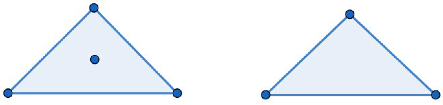
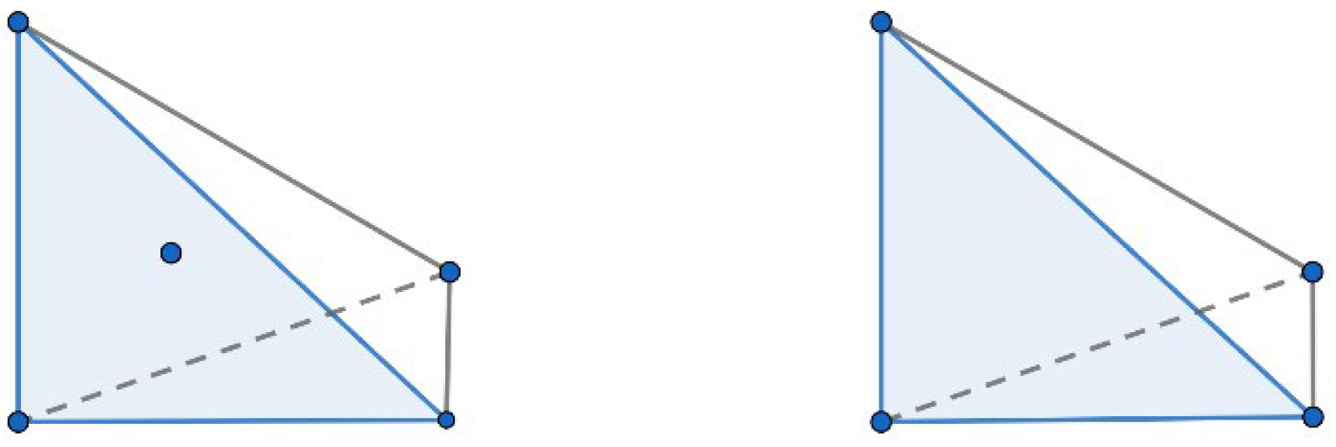
3. Mini-Element Method Approximation

Our goal here is to approximate the stationary Brinkman equations with general boundary conditions in a d-dimensional domain $(d=2,3)$ by using the mini-element method $P1-Bubble/P1$.

The mini-element method was first created by Arnold, Brezzi and Fortin [29]. The basic idea of the mini-element method is to add local functions called bubbles to correctly enrich the discrete velocity space in order to stabilize the unstable method $P1/P1$. Figure 1 and Figure 2 present the reference element of the mini-element $P1-Bubble/P1$ in two dimensions below and in three dimensions above.

Figure 1. Mini-element $P1-Bubble/P1$ in $2D$.

Figure 2. Mini-element $P1-Bubble/P1$ in $3D$.

Let $T_h$ be a triangulation of $\mathrm{\Omega }$; we consider the function $b\in H^1(T)$, which takes the value $1$ at the barycenter and zero at the boundary $\partial T$ of the reference triangle $T$ and verifies $0\le b\le 1$. Such a function is known as a bubble function. The space associated with the bubble is defined by

$$B_h=\{v_h\in C(\overline{\mathrm{\Omega }});v_h^T=x{b}^T,\forall T\in T_h\},$$

(22)

where $x$ is a real number.

We define the discrete function spaces

$${\mathrm{V}}_{ih}=\{v_h\in C(\overline{\mathrm{\Omega }}):v_h^T\in P_1(T);,\forall T\in T_h\},i=1,\dots ,d.$$

(23)

$${\mathrm{Q}}_h=\{q_h\in C(\overline{\mathrm{\Omega }}):q_h^T\in P_1(T);,\forall T\in T_h,{\displaystyle {\int }_{\mathrm{\Omega }}}{q}_{h}dx=0\},$$

(24)

where $P_1\left(T\right)$ is the set of all $1$ -order polynomials on triangle $T$.

And we set

$$X_{ih}={\mathrm{V}}_{ih}\oplus B_h,$$

(25)

$${\mathrm{X}}_h=X_{1h}\times X_{2h}\times \dots \times X_{dh}.$$

(26)

As a result, ${\mathrm{X}}_h\subset V$, the $P1-Bubble/P1$ finite-element approximation of problem $\left(8\right)$, will find $(u_h,p_h)\in {\mathrm{X}}_h\times {\mathrm{Q}}_h$ such that

$$\left\{\begin{array}{ll}a(u_h,v_h)+b(v_h,p_h)=F(v_h)& \forall v_h\in X_h,\\ b(q_h,u_h)=0& \forall q_h\in Q_h.\end{array}\right.$$

(27)

The velocity field $u_h$ and the pressure $p_h$ for a given triangle $T$ are approximated by linear combinations of the basis functions ${({\varphi }_i)}_{i=1,\dots ,d+1}$ in the form

$$u_h^T={\displaystyle \sum _{i=1}^{d+1}}{u}_i{\varphi }_i(x)+u_b{\varphi }_b(x),\hspace{1em}\hspace{1em}{p}_h^T={\displaystyle \sum _{i=1}^{d+1}}{p}_i{\varphi }_i(x),\hspace{1em}\hspace{1em}d=2,3$$

(28)

where $u_i$ and $p_i$ are nodal values of $u_h$ and $p_h$, while $u_b$ is the bubble value. The basis functions are defined by

$${\varphi }_1(x,y)=1-x-y,\hspace{1em}{\varphi }_2(x,y)=x,\hspace{1em}{\varphi }_3(x,y)=y,\hspace{1em}\hspace{1em}{\varphi }_b(x,y)=27{\varphi }_1(x,y){\varphi }_2(x,y){\varphi }_3(x,y)$$

if $d=2$ and

$$\begin{gathered} {\varphi }_1(x,y)=1-x-y-z,\hspace{1em}{\varphi }_2(x,y)=x,\hspace{1em}{\varphi }_3(x,y)=y,\hspace{1em}\hspace{1em}{\varphi }_4(x,y)=z, \\ {\varphi }_b(x,y)=256{\varphi }_1(x,y){\varphi }_2(x,y){\varphi }_3(x,y){\varphi }_4(x,y) \end{gathered}$$

if $d=3$.

We can rephrase system $\left(27\right)$ as a (large) square matrix problem with the vectors $U$ and $P$ as the unknowns. By consequence, we obtain the following algebraic form:

$$\left[\begin{array}{cc}A& B^t\\ B& 0\end{array}\right]\left[\begin{array}{c}U\\ P\end{array}\right]=\left[\begin{array}{c}F\\ 0\end{array}\right],$$

(29)

where the matrices $A$, $B$, and the vector $F$ are defined by

$$\begin{array}{l}A=(A_{ij}),A_{ij}={\displaystyle {\int }_{\mathrm{\Omega }}}\tilde{\mu }\nabla {\varphi }_i\nabla {\varphi }_{j}dx+{\displaystyle {\int }_{\mathrm{\Omega }}}{K}^{-1}\mu {\varphi }_i{\varphi }_j,dx+{\displaystyle {\int }_{\partial \mathrm{\Omega }}}{B}^{-1}{A}^{-1}{\varphi }_i{\varphi }_{j}d\sigma ,\\ i,j=1, \dots ,n_u.\\ B=(B_{kj}),B_{kj}=-{\displaystyle {\int }_{\mathrm{\Omega }}}{\partial }_1{\varphi }_k{\varphi }_j,dx-{\displaystyle {\int }_{\mathrm{\Omega }}}{\partial }_2{\varphi }_k{\varphi }_j,dx,k=1, \dots ,n_p \mathrm{and} \\ j=1, \dots ,n_u.\\ F=(F_i),F_i={\displaystyle {\int }_{\mathrm{\Omega }}}f{\varphi }_i,dx+{\displaystyle {\int }_{\partial \mathrm{\Omega }}}{B}^{-1}g{\varphi }_i,d\sigma ,i=1, \dots ,n_u.\end{array}$$

To solve the large system we can be use the Uzawa conjugate gradient algorithm [32,33,34].

4. Stability and a Priori Error Estimates

In this section, we will establish the stability and a priori estimate for the pressure and the velocity of our problem.

Lemma 1.

There is a constant  $c_4\succ 0$ independent from the mesh parameter h such that

$$\underset{v_h\in {\mathrm{X}}_h}{{\displaystyle \sup }}\frac{b(v_h,q_h)}{\parallel v_h{\parallel }_{\mathrm{V}}}\ge C_4\parallel q_h{\parallel }_{0,\mathrm{\Omega }},\hspace{1em}\forall q_h\in {\mathrm{Q}}_h.$$

(30)

Proof of Lemma 1.

This Lemma can be established by the same proof of Lemma 2 in [35]. □

Theorem 3.

For any  $(w_h,s_h)\in {\mathrm{X}}_h\times {\mathrm{Q}}_h$ there is a constant  $c_5\succ 0$ independent from the mesh parameter  $h$ such that

$$\underset{(v_h,q_h)\in {\mathrm{X}}_h\times {\mathrm{Q}}_h}{{\displaystyle \sup }}\frac{a(w_h,v_h)+d(s_h,q_h)}{\parallel v_h{\parallel }_V+\parallel q_h{\parallel }_{0,\mathrm{\Omega }}}\ge C_5\left(\parallel w_h{\parallel }_{\mathrm{V}}+\parallel s_h{\parallel }_{0,\mathrm{\Omega }}\right),$$

(31)

where $d(s_h,q_h)={\displaystyle {\int }_{\mathrm{\Omega }}}{s}_h{q}_h,dx,\hspace{1em}\forall (q_h,s_h)\in {\mathrm{Q}}_h^2.$

Proof of Theorem 3.

For any $(w_h,s_h)$ in $X_h\times {\mathrm{Q}}_h$ we have:

Firstly,

$$\underset{(v_h,q_h)\in {\mathrm{X}}_h\times {\mathrm{Q}}_h}{{\displaystyle \sup }}\frac{a(w_h,v_h)+d(s_h,q_h)}{\parallel v_h{\parallel }_V+\parallel q_h{\parallel }_{0,\mathrm{\Omega }}}\ge \frac{a(w_h,w_h)+d(s_h,0)}{\parallel w_h{\parallel }_V+\parallel 0{\parallel }_{0,\mathrm{\Omega }}}\ge \parallel w_h{\parallel }_{\mathrm{V}},$$

(32)

On the other hand,

$$\underset{(v_h,q_h)\in {\mathrm{X}}_h\times {\mathrm{Q}}_h}{{\displaystyle \sup }}\frac{a(w_h,v_h)+d(s_h,q_h)}{\parallel v_h{\parallel }_V+\parallel q_h{\parallel }_{0,\mathrm{\Omega }}}\ge \frac{a(w_h,0)+d(s_h,s_h)}{\parallel 0{\parallel }_V+\parallel s_h{\parallel }_{0,\mathrm{\Omega }}}\ge \parallel s_h{\parallel }_{0,\mathrm{\Omega }},$$

(33)

by combining these inequalities in Equations (32)–(33), we obtain the result Equation (31), of which the constant is $C_5=\frac{1}{2}$. □

Now, we will introduce and demonstrate the a priori estimate error.

Theorem 4.

Let  $(u,p)$ be the solution of (1)–(2), and  $(u_h,p_h)$ be the solution of  $\left(27\right).$ Then the following error estimate holds

$$\parallel u-u_h{\parallel }_V+\parallel p-p_h{\parallel }_{0,\mathrm{\Omega }}\le C \left\{\underset{{}_{v\in X_h}}{inf}\parallel u-v{\parallel }_V+\underset{q\in Q_h}{inf}\parallel p-q{\parallel }_{0,\mathrm{\Omega }}\right\},$$

(34)

where C is a constant independent of the mesh size $h$.

Proof of Theorem 4.

Using the triangle inequality, we have

$$\parallel u-u_h{\parallel }_V+\parallel p-p_h{\parallel }_{0,\mathrm{\Omega }}\le \parallel u-v{\parallel }_V+\parallel p-\mathrm{q}{\parallel }_{0,\mathrm{\Omega }}+\parallel u_h-v{\parallel }_V+\parallel p_h-q{\parallel }_{0,\mathrm{\Omega }},$$

(35)

from Equation (31) there exists $\left(w,q\right)\in X_h\times Q_h$ with

$$\parallel w{\parallel }_{X_h}+\parallel q{\parallel }_{0,\mathrm{\Omega }}\le {\gamma }_1,$$

(36)

such that

$$\parallel u_h-v{\parallel }_{\mathrm{V}}+\parallel p_h-q{\parallel }_{0,\mathrm{\Omega }}\le a(u_h-v,w)+b(w,p_h-q).$$

(37)

Since

$$a(u-v,w)+b(w,p-q)=a(u_h-v,w)+b(w,p_h-q),$$

(38)

and by using the Schwartz inequality we obtain $·$

$$\begin{gathered} a(u-v,w)+b(w,p-q)={\displaystyle {\int }_{\mathrm{\Omega }}}\tilde{\mu }\nabla (u-v)\nabla w,dx+{\displaystyle {\int }_{\mathrm{\Omega }}}{K}^{-1}\mu (u-v).w,dx \\ +{\displaystyle {\int }_{\mathrm{\Gamma }}}{B}^{-1}{A}^{-1}(u-v)·w,d\sigma +{\displaystyle {\int }_{\mathrm{\Omega }}}(p-q)\nabla ·w,dx \\ \le {\tilde{\mu }}_0\parallel \nabla (u-v){\parallel }_{0,\mathrm{\Omega }}\parallel \nabla w{\parallel }_{0,\mathrm{\Omega }}+k_2{\mu }_0\parallel u-v{\parallel }_{0,\mathrm{\Omega }}\parallel w{\parallel }_{0,\mathrm{\Omega }} \\ +b_2{a}_2\parallel u-v{\parallel }_{0,\mathrm{\Gamma }}\parallel w{\parallel }_{0,\mathrm{\Gamma }}+\parallel p-q{\parallel }_{0,\mathrm{\Omega }}\parallel \nabla w{\parallel }_{0,\mathrm{\Omega }} \\ \le C_6\parallel u-v{\parallel }_{\mathrm{V}}\parallel w{\parallel }_{\mathrm{V}}+C_7\parallel p-q{\parallel }_{0,\mathrm{\Omega }}\parallel w{\parallel }_{\mathrm{V}} \\ \le C(\parallel u-v{\parallel }_{\mathrm{V}}+\parallel p-q{\parallel }_{0,\mathrm{\Omega }}) \end{gathered}$$

by the consistency, we have the result Equation (34). □

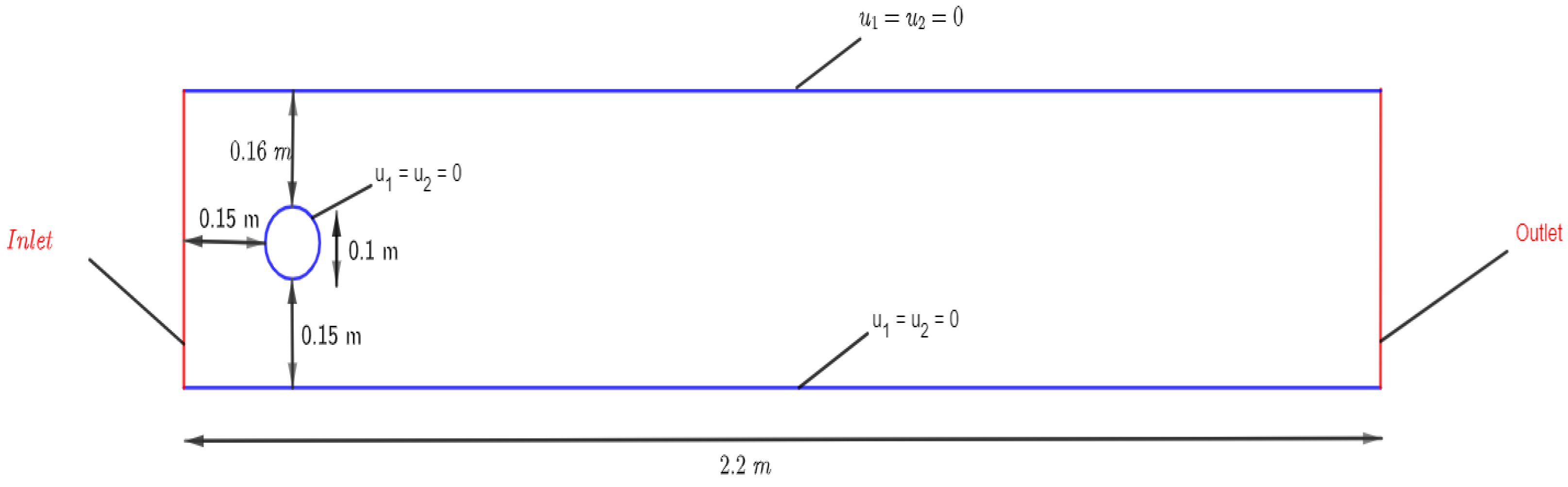
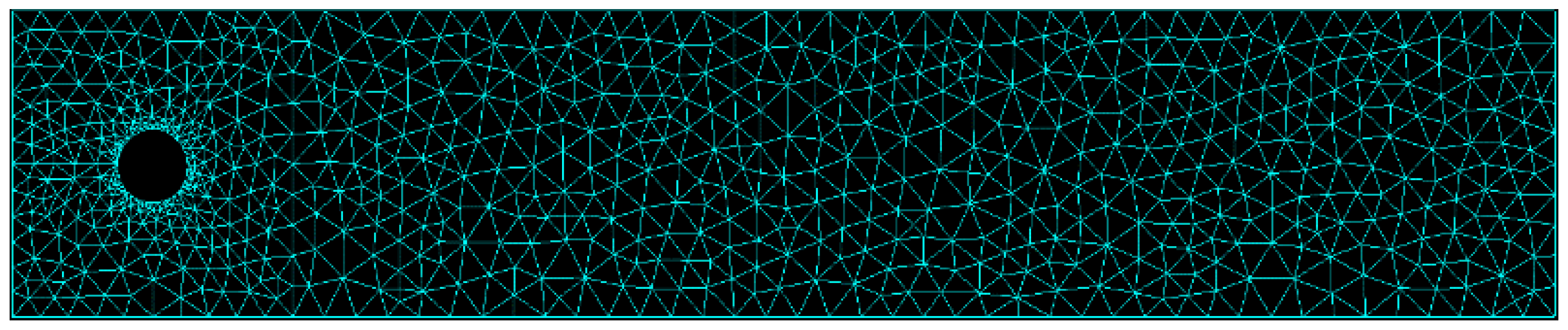
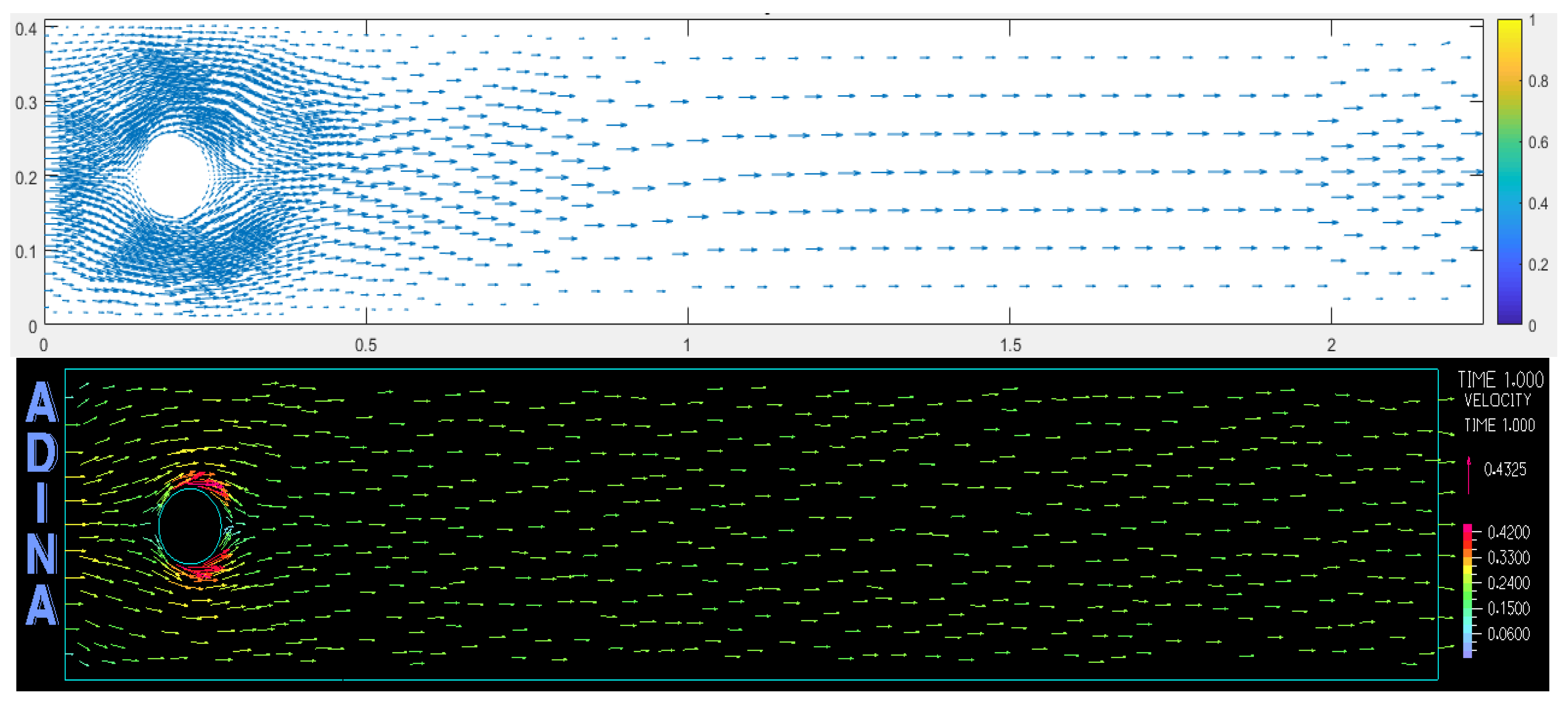
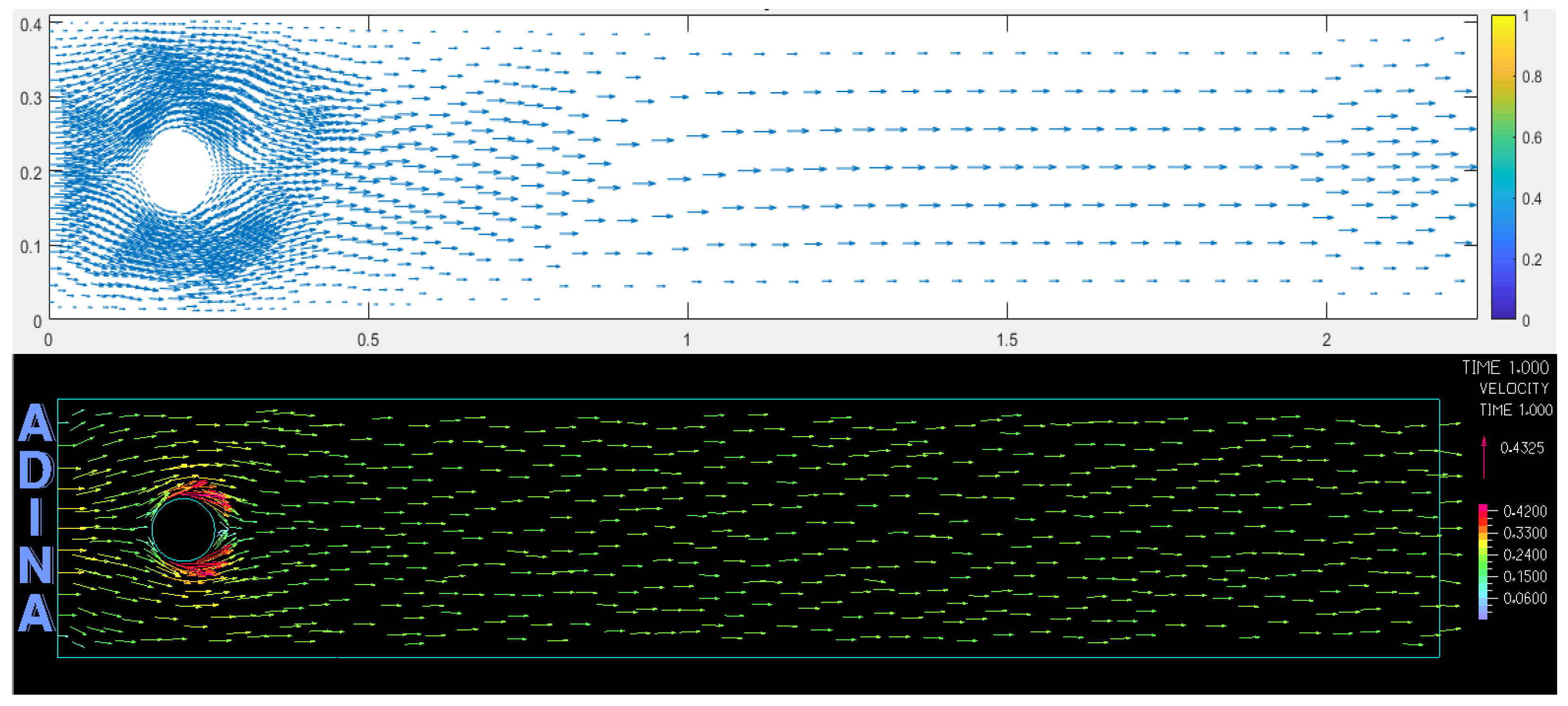
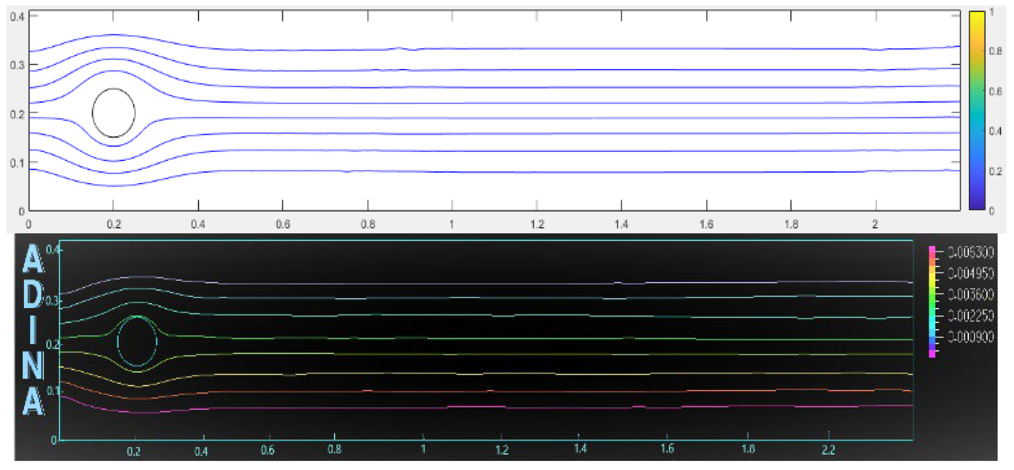
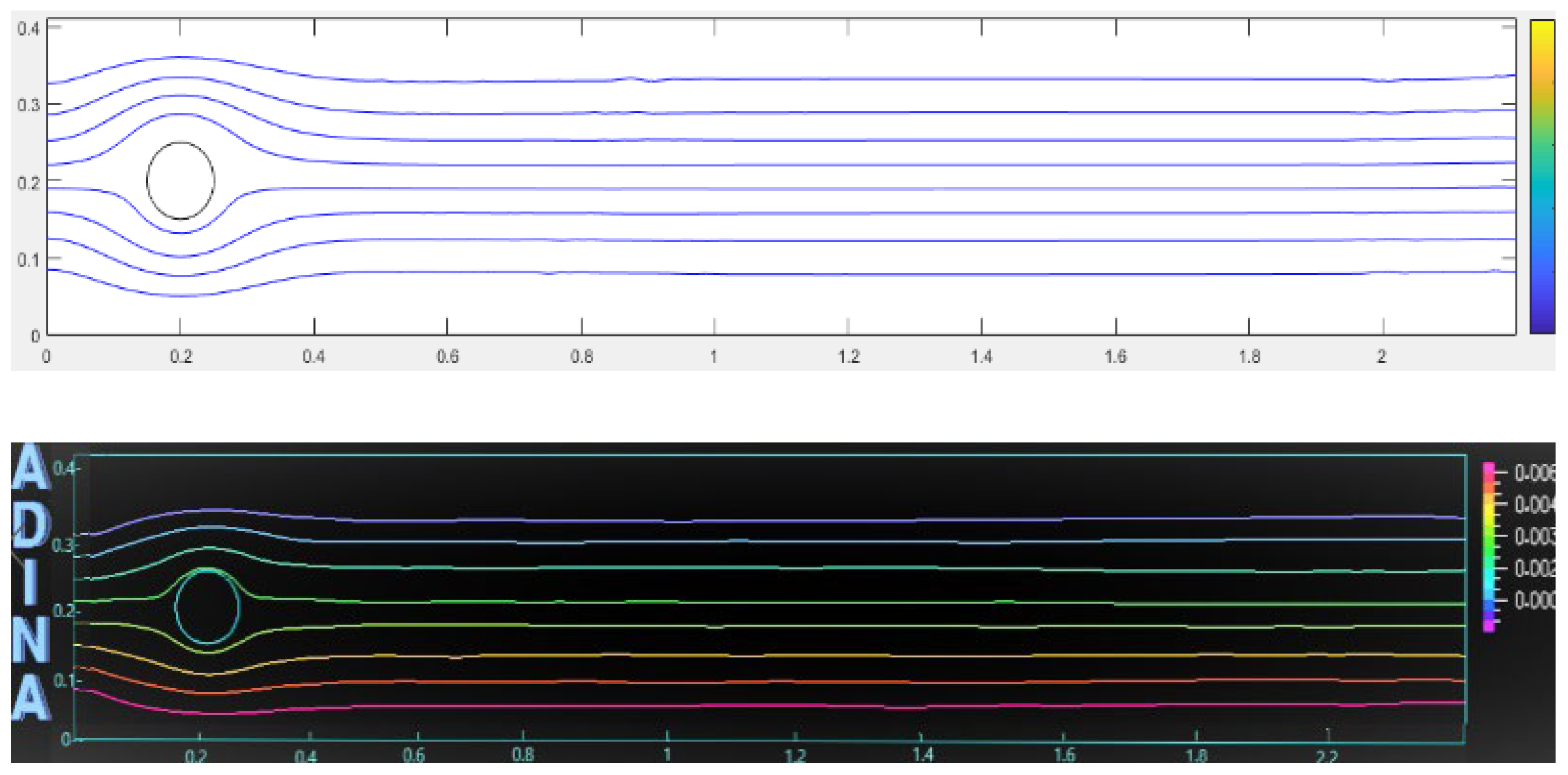
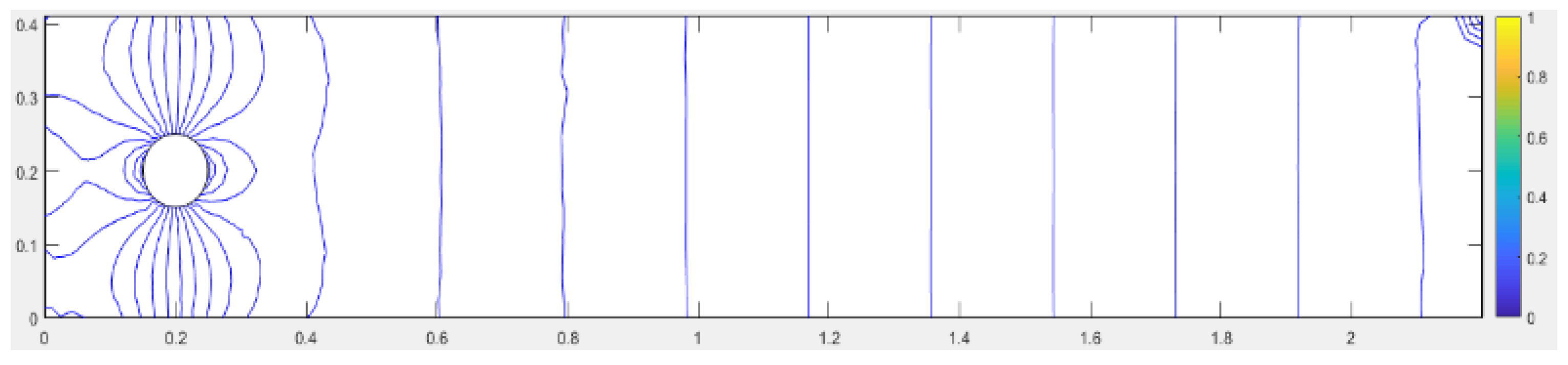
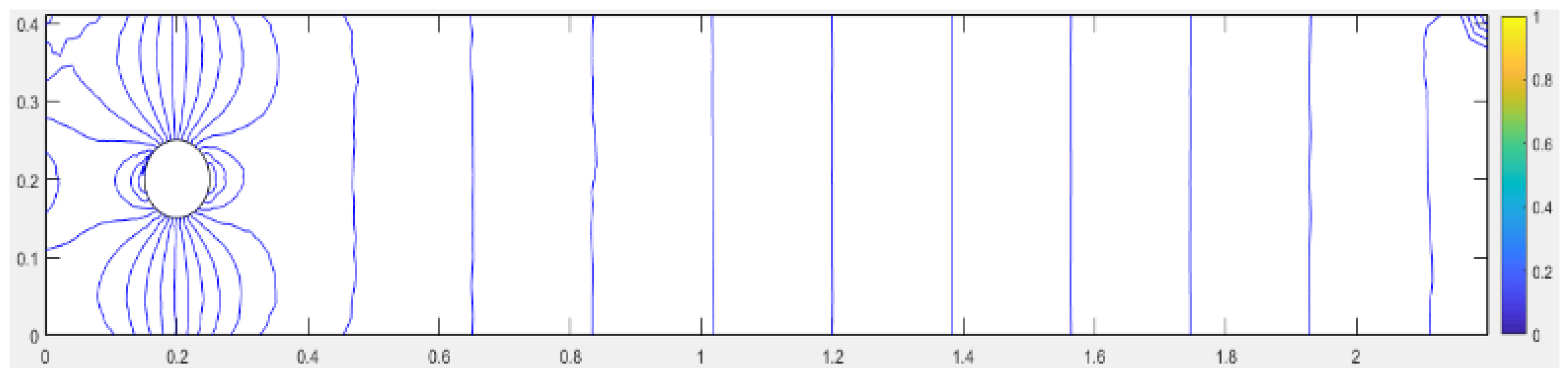
5. Numerical Simulation

In this section, some numerical results were obtained by programming the mini-element method in MATLAB and we compare these obtained results with those constructed from the ADINA system. Using our solver, we ran two test problems regarding the flow around a cylinder; our tests were focused on the change in the value of the diagonal coefficients of the permeability matrix. For both of the tests, the domain considered in the simulation experiment is the one studied by Schäfer et al. in [36] for two dimensions.

Example 1.

In this test, we performed simulations for the flow around a cylinder (Figure 3) by the change in the values of the coefficients ${\alpha }_1$and ${\alpha }_2$ of the matrix ${\mathrm{K}}^{-1}$ defined as ${\mathrm{K}}^{-1}=\left(\begin{array}{cc}{\alpha }_1& 0\\ 0& {\alpha }_2\end{array}\right),$where ${\alpha }_1$and ${\alpha }_2$ are two positive real numbers.

Figure 3. The simulated geometry of the cylinder and notations for the boundary conditions of the 2D test case.

The Figure 3 presents the domain geometry of the cylinder. The channel height is $H=0.41 \mathrm{m}$and the diameter is $D=0.1 \mathrm{m}$.

Next, we present the simulation made with the MATLAB software with the validation tests performed by the ADINA system. We used the Newtonian viscosity and dynamic viscosity, $\mu =\tilde{\mu }=1$. For the boundary conditions, we considered the boundary defined in [36], for which we considered the matrix $A^{-1}$and $B$defined by 

$$A^{-1}=\left(\begin{array}{cc}1& 0\\ 0& 1\end{array}\right), B=\left(\begin{array}{cc}{10}^{-6}& 0\\ 0& {10}^{-6}\end{array}\right).$$

(39)

The Figure 4 shows the ADINA created domain mesh upon which the various tests are based.

Figure 4. Mesh sample of domain created by the ADINA system.

Firstly, we present in Figure 5 and Figure 6 the velocity field of our problem $\left(1\right) and \left(2\right)$ in the following different cases  ${\alpha }_1={\alpha }_2={10}^{-6}$ and  ${\alpha }_1={10}^{-4}$,  ${\alpha }_2=1$.

Figure 5. Velocity vector solution by $P1-Bubble/P1$ (above) and velocity vector solution computed by the ADINA system (below) with ${\alpha }_1={\alpha }_2={10}^{-6}$.

Figure 6. Velocity vector solution by $P1-Bubble/P1$ (above) and velocity vector solution computed by the ADINA system (below) with ${\alpha }_1={10}^{-4}$, ${\alpha }_2=1$.

The streamlines were derived from the velocity solution by numerically solving the Poisson equation with a zero Dirichlet boundary condition. Figure 7 and Figure 8 present the streamlines in the following different cases: ${\alpha }_1={\alpha }_2={10}^{-6} and$${\alpha }_1={10}^{-4}$, ${\alpha }_2=1.$

Figure 7. Solution computed with MATLAB (above) and with the ADINA system (below). The plots show the streamlines associated with a ${\alpha }_1={\alpha }_2={10}^{-6}$.

Figure 8. Solution computed with MATLAB (above) and with the ADINA system (below). The plots show the streamlines associated with a ${\alpha }_1={10}^{-4}$, ${\alpha }_2=1$.

Isobar lines: Figure 9 and Figure 10 present the isobar lines in the following different cases ${\alpha }_1={\alpha }_2={10}^{-6}$ and  ${\alpha }_1={10}^{-4}$,  ${\alpha }_2=1$.

Figure 9. Isobar lines, ${\alpha }_1={\alpha }_2={10}^{-6}$.

Figure 10. Isobar lines, ${\alpha }_1={10}^{-4}$, ${\alpha }_2=1$.

In the previous example, the two-dimensional flow past a circular cylinder was simulated for varied permeability tensor ${\mathrm{K}}^{-1}$. The objective of the present simulation was to investigate the solution of Brinkman’s equations by using the mini-elements method $P1-Bubble/P1$. Our simulation focused on two tests with deferent values for ${\mathrm{K}}^{-1}$such that the first was ${\alpha }_1={\alpha }_2={10}^{-6}$and the second was ${\alpha }_1={10}^{-4}$, ${\alpha }_2=1$. The computations with MATLAB and the ADINA system led to very similar results.

Example 2.

We consider the stationary Brinkman problem (1) in $\mathrm{\Omega }=[0;1]\times [0;1],$with  $\mu =1$ and  $\tilde{\mu }=1$, the function  $f$ on the right-hand side in (1) is adjusted so that the exact solution is

$$u_1(x,y)=x^2(\frac{x}{3}-\frac{1}{2}),u_2(x,y)=xy(1-x),$$

(40)

for the velocity, and we take the pressure to be

$$p(x,y)=x^2-\frac{1}{3},$$

(41)

with the boundary conditions  $\left[\begin{array}{cc}1& 0\\ 0& 1\end{array}\right]\left[\begin{array}{c}{u}_1\\ u_2\end{array}\right]+\left[\begin{array}{cc}{10}^{-6}& 0\\ 0& {10}^{-6}\end{array}\right]\left(\nabla u-pI\right).n=0\mathrm{on}\mathrm{\Gamma }$.

The domain $\mathrm{\Omega }$is first discretized by a uniform mesh of size $h=1/16$(289 nodes and 512 triangles in the fine mesh). This initial mesh is successively refined to produce meshes with sizes $2^{-5}$, $2^{-6}$, $2^{-7}$, $2^{-8}$, $2^{-9}$and $2^{-10}.$We report in Table 1 the convergence rates and the distances $\parallel u-u_h{\parallel }_{H^1}$and $\parallel u-u_h{\parallel }_{L^2}$between the exact solution $\left(40\right) and \left(41\right)$and approximate solution. For this test, we took two values of ${\mathrm{K}}^{-1}$, and we noticed that these norms were converging to zero.

Table 1. Numerical error and convergence rates for example 2.

Permeability	Mesh Size	${\Vert \mathit{u}-{\mathit{u}}_{\mathit{h}}\Vert }_{\mathit{L}\mathbf{2}}$	Rate	${\Vert \mathit{u}-{\mathit{u}}_{\mathit{h}}\Vert }_{{\mathit{H}}^{\mathbf{1}}}$	Rate
${\mathrm{K}}^{-1}=\left(\begin{array}{cc}1& 0\\ 0& 1\end{array}\right)$	$2^{-5}$	2.58490367 × 10−3		7.30459072 × 10−2
	$2^{-6}$	7.29374932 × 10−4	1.23	3.65242949 × 10−2	1.26
	$2^{-7}$	2.00944198 × 10−4	1.12	1.82662182 × 10−2	1.20
	$2^{-8}$	5.45035935 × 10−5	1.20	9.13565045 × 10−3	1.17
	$2^{-9}$	1.46182239 × 10−5	1.13	4.56876194 × 10−3	1.14
	$2^{-10}$	6.34523145 × 10−6	1.07	8.5232210 × 10−4	1.31
${\mathrm{K}}^{-1}=\left(\begin{array}{cc}{10}^4& 0\\ 0& {10}^4\end{array}\right)$	$2^{-5}$	9.79901277 × 10−2		1.71655622 ×100
	$2^{-6}$	5.71231633 × 10−2	1.23	1.13006936 × 100	1.30
	$2^{-7}$	2.10804196 × 10−2	1.34	4.88759130 × 10−1	1.29
	$2^{-8}$	5.96212978 × 10−3	1.32	1.82645760 × 10−1	1.30
	$2^{-9}$	1.54001284 × 10−3	1.26	6.50585157 × 10−2	1.27
	$2^{-10}$	3.88183415 × 10−4	1.21	2.29466805 × 10−2	1.31

Since the assembly process is essentially based on the number of elements, we expect that the time to assemble the matrices will increase by approximately the same factor. We can see that Table 2 shows an almost linear optimal time-scaling for our implementation.

Table 2. CPU time in seconds for example 2 with ${\mathrm{K}}^{-1}=\left(\begin{array}{cc}1& 0\\ 0& 1\end{array}\right)$.

Mesh Size	$2^{-5}$	$2^{-6}$	$2^{-7}$	$2^{-8}$	$2^{-9}$	$2^{-10}$
CPU Time (s)	0.4521	0.1894	0.5811	2.4645	14.1669	26.20

6. Conclusions

We were interested in this work on the numeric solution of this equation in a heterogeneous porous media with a permeability tensor. In this study, we used the discretization of the mini-element method $P1-Bubble/P1$. We established the stability and a priori error estimate for this approximation. The numerical and bidimensional simulations are presented and show the accuracy and efficiency of the proposed finite-element method.

References

- Brinkman, H.C. On the Permeability of Media Consisting of Closely Packed Porous Particles. Flow Turbul. Combust. 1949, 1, 81–86. [Google Scholar] [CrossRef]
- Iliev, O.; Lazarov, R.; Willems, J. Variational Multiscale Finite Element Method for Flows in Highly Porous Media. Multiscale Modeling Simul. 2011, 9, 1350–1372. [Google Scholar] [CrossRef]
- Kanschat, G.; Lazarov, R.; Mao, Y. Geometric Multigrid for Darcy and Brinkman Models of Flows in Highly Heterogeneous Porous Media: A Numerical Study. J. Comput. Appl. Math. 2017, 310, 174–185. [Google Scholar] [CrossRef]
- Koplik, J.; Levine, H.; Zee, A. Viscosity Renormalization in the Brinkman Equation. Phys. Fluids 1983, 26, 2864–2870. [Google Scholar] [CrossRef]
- Angot, P. Analysis of Singular Perturbations on the Brinkman Problem for Fictitious Domain Models of Viscous Flows. Math. Methods Appl. Sci. 1999, 22, 1395–1412. [Google Scholar] [CrossRef]
- Shahnazari, M.R.; Moosavi, M.H. Investigation of Nonlinear Fluid Flow Equation in a Porous Media and Evaluation of Convection Heat Transfer Coefficient, By Taking the Forchheimer Term into Account. Int. J. Theor. Appl. Mech. 2022, 7, 12–17. [Google Scholar] [CrossRef]
- Shahnazari, M.R.; Hagh, M.Z.B. Theoretical and Experimental Investigation of the Channeling Effect in Fluid Flow through Porous Media. J. Porous Media 2005, 8, 115–124. [Google Scholar] [CrossRef]
- Shahnazari, M.R.; Ahmadi, Z.; Masooleh, L.S. Perturbation Analysis of Heat Transfer and a Novel Method for Changing the Third Kind Boundary Condition into the First Kind. J. Porous Media 2017, 20, 449–460. [Google Scholar] [CrossRef]
- Iasiello, M.; Bianco, N.; Chiu, W.K.; Naso, V. Anisotropic Convective Heat Transfer in Open-Cell Metal Foams: Assessment and Correlations. Int. J. Heat Mass Transf. 2020, 154, 119682. [Google Scholar] [CrossRef]
- Iasiello, M.; Bianco, N.; Chiu, W.K.S.; Naso, V. Anisotropy Effects on Convective Heat Transfer and Pressure Drop in Kelvin’s Open-Cell Foams. J. Phys. Conf. Ser. 2017, 923, 012035. [Google Scholar] [CrossRef]
- Amani, Y.; Takahashi, A.; Chantrenne, P.; Maruyama, S.; Dancette, S.; Maire, E. Thermal Conductivity of Highly Porous Metal Foams: Experimental and Image Based Finite Element Analysis. Int. J. Heat Mass Transf. 2018, 122, 1–10. [Google Scholar] [CrossRef]
- Shah, N.A.; Wakif, A.; El-Zahar, E.R.; Ahmad, S.; Yook, S.-J. Numerical Simulation of a Thermally Enhanced EMHD Flow of a Heterogeneous Micropolar Mixture Comprising (60%)-Ethylene Glycol (EG),(40%)-Water (W), and Copper Oxide Nanomaterials (CuO). Case Stud. Therm. Eng. 2022, 35, 102046. [Google Scholar] [CrossRef]
- Wakif, A.; Chamkha, A.; Animasaun, I.L.; Zaydan, M.; Waqas, H.; Sehaqui, R. Novel Physical Insights into the Thermodynamic Irreversibilities within Dissipative EMHD Fluid Flows Past over a Moving Horizontal Riga Plate in the Coexistence of Wall Suction and Joule Heating Effects: A Comprehensive Numerical Investigation. Arab. J. Sci. Eng. 2020, 45, 9423–9438. [Google Scholar] [CrossRef]
- Nayak, M.K.; Wakif, A.; Animasaun, I.L.; Alaoui, M. Numerical Differential Quadrature Examination of Steady Mixed Convection Nanofluid Flows over an Isothermal Thin Needle Conveying Metallic and Metallic Oxide Nanomaterials: A Comparative Investigation. Arab. J. Sci. Eng. 2020, 45, 5331–5346. [Google Scholar] [CrossRef]
- Wakif, A. A Novel Numerical Procedure for Simulating Steady MHD Convective Flows of Radiative Casson Fluids over a Horizontal Stretching Sheet with Irregular Geometry under the Combined Influence of Temperature-Dependent Viscosity and Thermal Conductivity. Math. Probl. Eng. 2020, 2020, 1675350. [Google Scholar] [CrossRef]
- Ashraf, M.U.; Qasim, M.; Wakif, A.; Afridi, M.I.; Animasaun, I.L. A Generalized Differential Quadrature Algorithm for Simulating Magnetohydrodynamic Peristaltic Flow of Blood-Based Nanofluid Containing Magnetite Nanoparticles: A Physiological Application. Numer. Methods Partial. Differ. Equ. 2022, 38, 666–692. [Google Scholar] [CrossRef]
- Wakif, A.; Zaydan, M.; Alshomrani, A.S.; Muhammad, T.; Sehaqui, R. New Insights into the Dynamics of Alumina-(60% Ethylene Glycol+ 40% Water) over an Isothermal Stretching Sheet Using a Renovated Buongiorno’s Approach: A Numerical GDQLLM Analysis. Int. Commun. Heat Mass Transf. 2022, 133, 105937. [Google Scholar] [CrossRef]
- Xiong, Q.; Hajjar, A.; Alshuraiaan, B.; Izadi, M.; Altnji, S.; Shehzad, S.A. State-of-the-Art Review of Nanofluids in Solar Collectors: A Review Based on the Type of the Dispersed Nanoparticles. J. Clean. Prod. 2021, 310, 127528. [Google Scholar] [CrossRef]
- Ramesh, G.K.; Shehzad, S.A.; Izadi, M. Thermal Transport of Hybrid Liquid over Thin Needle with Heat Sink/Source and Darcy–Forchheimer Porous Medium Aspects. Arab. J. Sci. Eng. 2020, 45, 9569–9578. [Google Scholar] [CrossRef]
- Huu-Quan, D.; Mohammad Rostami, A.; Shokri Rad, M.; Izadi, M.; Hajjar, A.; Xiong, Q. 3D Numerical Investigation of Turbulent Forced Convection in a Double-Pipe Heat Exchanger with Flat Inner Pipe. Appl. Therm. Eng. 2021, 182, 116106. [Google Scholar] [CrossRef]
- Ern, A. Aide-Mémoire Des Éléments Finis; Dunod: Malakoff, France, 2005. [Google Scholar]
- Raviart, P.-A. Introduction à L’Analyse Numérique Des Équations Aux Dérivées Partielles; Dunod: Malakoff, France, 1983. [Google Scholar]
- Boffi, D.; Brezzi, F.; Fortin, M. Mixed Finite Element Methods and Applications; Springer: Berlin/Heidelberg, Germany, 2013; Volume 44. [Google Scholar]
- El Moutea, O.; El Amri, H.; El Akkad, A. Mixed Finite Element Method for Flow of Fluid in Complex Porous Media with a New Boundary Condition. Comput. Sci. 2020, 15, 413–431. [Google Scholar]
- John, V. Finite Element Methods for Incompressible Flow Problems; Springer: Berlin/Heidelberg, Germany, 2016; Volume 51. [Google Scholar]
- Elakkad, A.; Elkhalfi, A.; Guessous, N. An a Posteriori Error Estimate for Mixed Finite Element Approximations of the Navier-Stokes Equations. J. Korean Math. Soc. 2011, 48, 529–550. [Google Scholar] [CrossRef]
- Tinsley Oden, J.; Wu, W.; Ainsworth, M. An a Posteriori Error Estimate for Finite Element Approximations of the Navier-Stokes Equations. Comput. Methods Appl. Mech. Eng. 1994, 111, 185–202. [Google Scholar] [CrossRef]
- Hannukainen, A.; Juntunen, M.; Stenberg, R. Computations with Finite Element Methods for the Brinkman Problem. Comput. Geosci. 2011, 15, 155–166. [Google Scholar] [CrossRef]
- Arnold, D.N.; Brezzi, F.; Fortin, M. A Stable Finite Element for the Stokes Equations. Calcolo 1984, 21, 337–344. [Google Scholar] [CrossRef]
- Brezzi, F.; Fortin, M. Mixed and Hybrid Finite Element Methods; Springer Science & Business Media: Berlin/Heidelberg, Germany, 2012; Volume 15. [Google Scholar]
- Koubaiti, O.; Elkhalfi, A.; El-Mekkaoui, J.; Mastorakis, N. Solving the Problem of Constraints Due to Dirichlet Boundary Conditions in the Context of the Mini Element Method. Int. J. Mech. 2020, 14, 12–21. [Google Scholar]
- Bramble, J.H.; Pasciak, J.E.; Vassilev, A.T. Analysis of the Inexact Uzawa Algorithm for Saddle Point Problems. SIAM J. Numer. Anal. 1997, 34, 1072–1092. [Google Scholar] [CrossRef]
- Hackbusch, W. Iterative Solution of Large Sparse Systems of Equations; Springer: Berlin/Heidelberg, Germany, 1994; Volume 95. [Google Scholar]
- Koko, J. Efficient MATLAB Codes for the 2D/3D Stokes Equation with the Mini-Element. Informatica 2019, 30, 243–268. [Google Scholar] [CrossRef]
- Juntunen, M.; Stenberg, R. Analysis of Finite Element Methods for the Brinkman Problem. Calcolo 2010, 47, 129–147. [Google Scholar] [CrossRef]
- Schäfer, M.; Turek, S.; Durst, F.; Krause, E.; Rannacher, R. Benchmark Computations of Laminar Flow around a Cylinder. In Flow Simulation with High-Performance Computers II; Springer: Berlin/Heidelberg, Germany, 1996; pp. 547–566. [Google Scholar]
Publisher’s Note: MDPI stays neutral with regard to jurisdictional claims in published maps and institutional affiliations. |
© 2022 by the authors. Licensee MDPI, Basel, Switzerland. This article is an open access article distributed under the terms and conditions of the Creative Commons Attribution (CC BY) license (https://creativecommons.org/licenses/by/4.0/).