
Rain Rendering and Construction of Rain Vehicle Color-24 Dataset

Abstract
:1. Introduction
- (1)
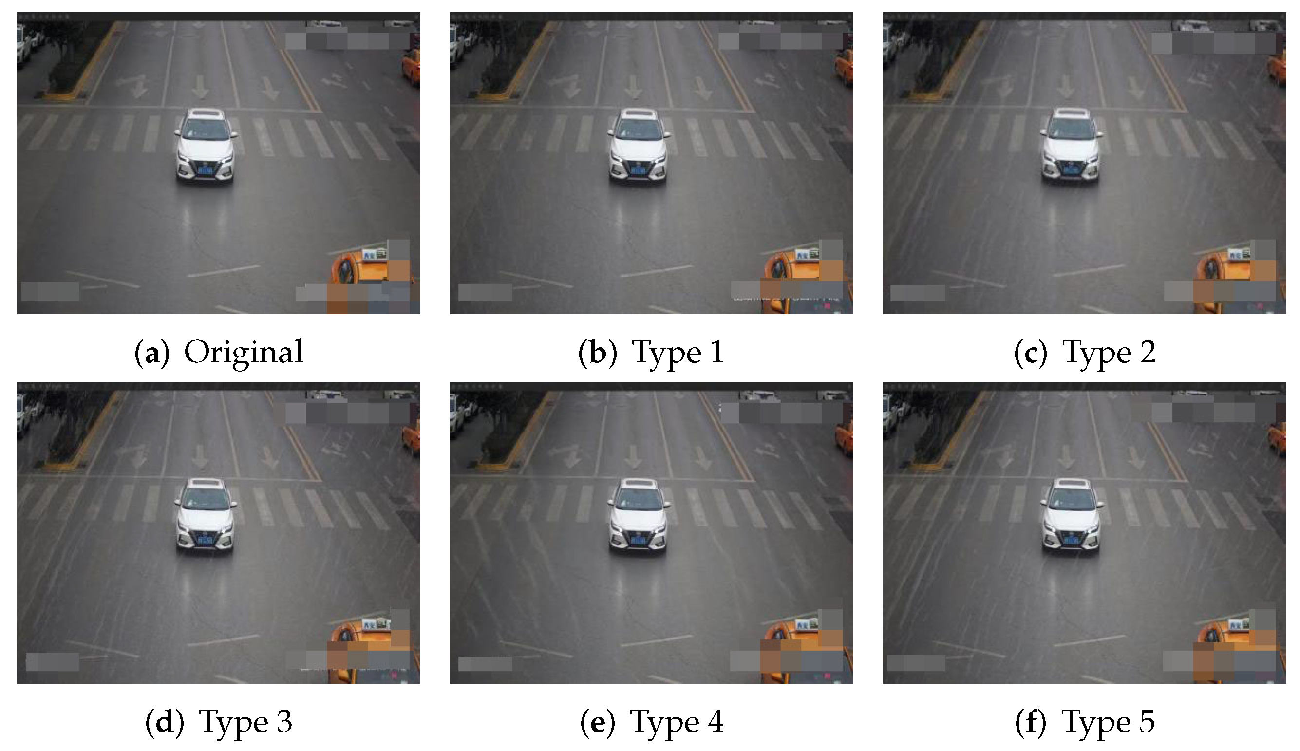
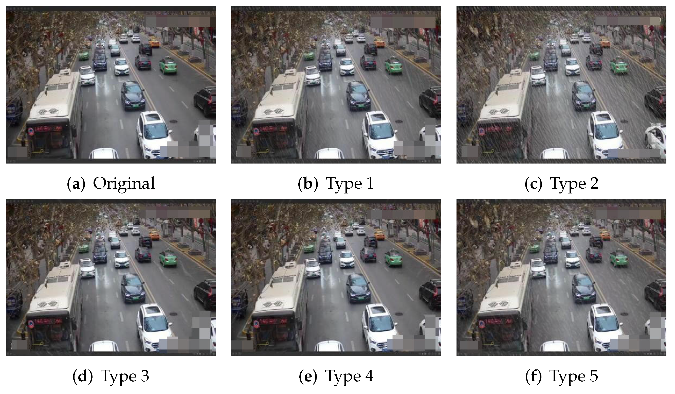
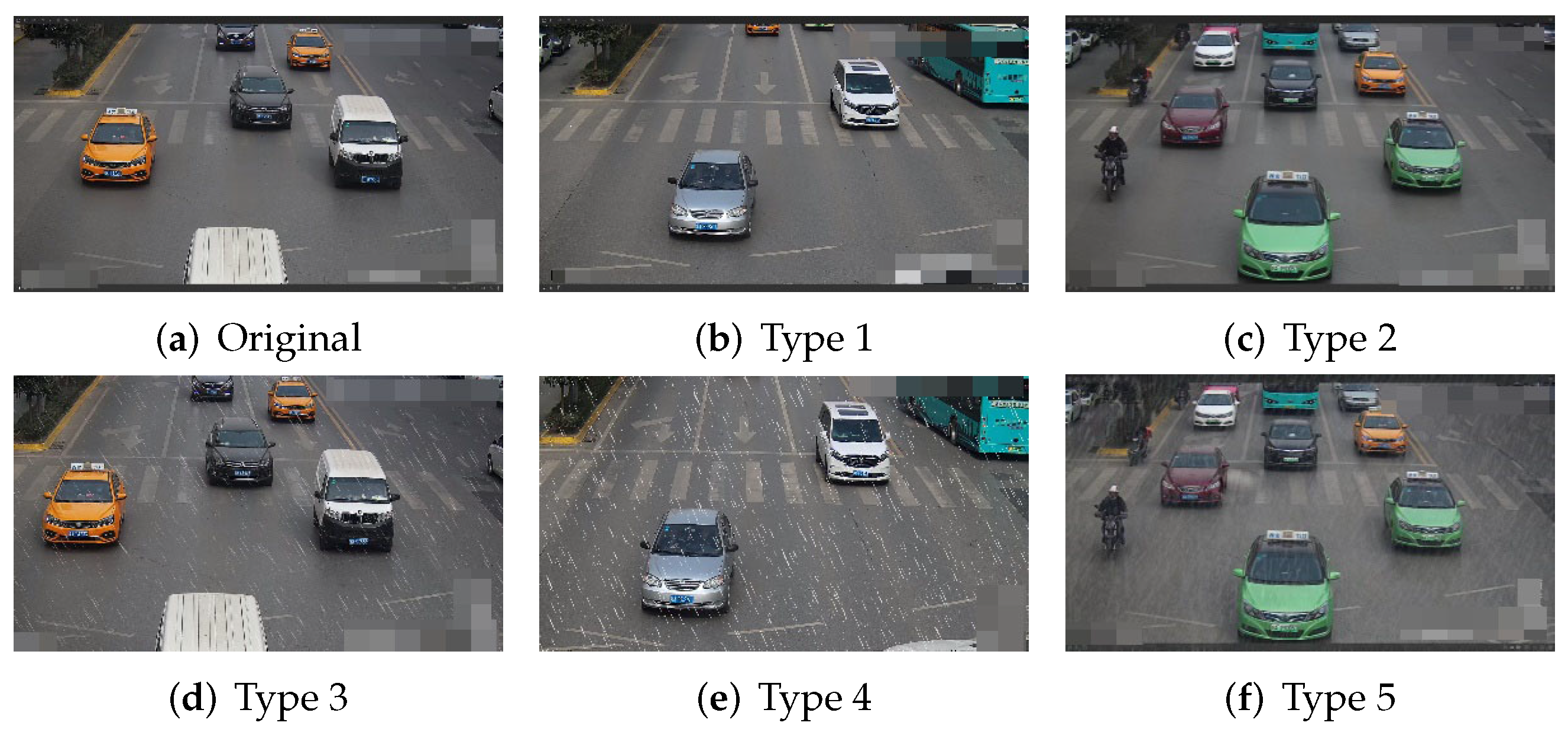
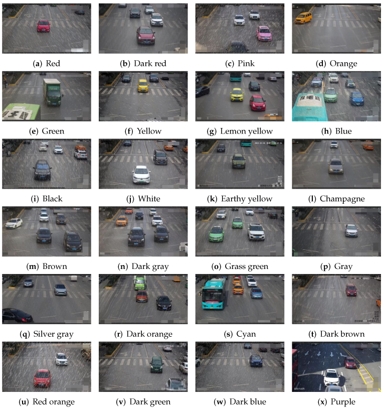
- This paper constructs the -24 dataset by rain-image-rendering technology, in order to address the specific task of the vehicle-color fine recognition. Both model-based and data-driven-based rendering are used: the former synthesizes 300 images by to form one subset in which clean background images are from the -24; the latter, i.e., the network, synthesizes 8000 vehicle images to form another subset in which clean background images are also from the -24;
- (2)
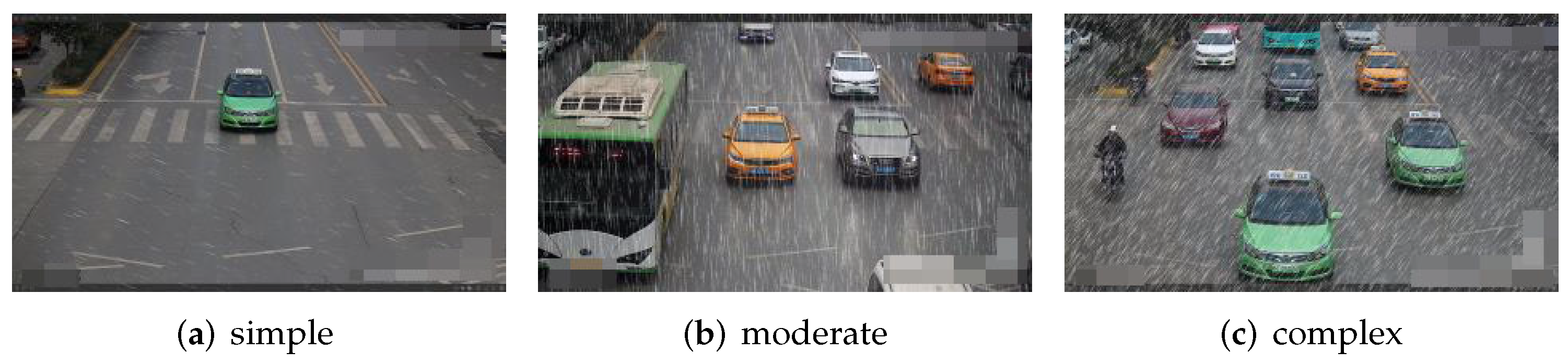
- This dataset helps to increase the performance of vehicle-color recognition methods on rainy days since the -24 dataset consists paired vehicle-color rain images with various rain patterns;
- (3)
- We improve the performances of existing algorithms for vehicle-color identification in rainy conditions. Vehicle-color identification plays a key role in intelligent traffic management and criminal investigation. However, existing algorithms are typically trained on the datasets collected in good weather conditions, which suffer from poor performance in poor weather conditions, such as rainy weather. In this paper, we show that our newly constructed dataset is critically beneficial to the performances of existing algorithms for vehicle-color identification in rainy conditions.
2. Related Work
2.1. Photoshop () Technology
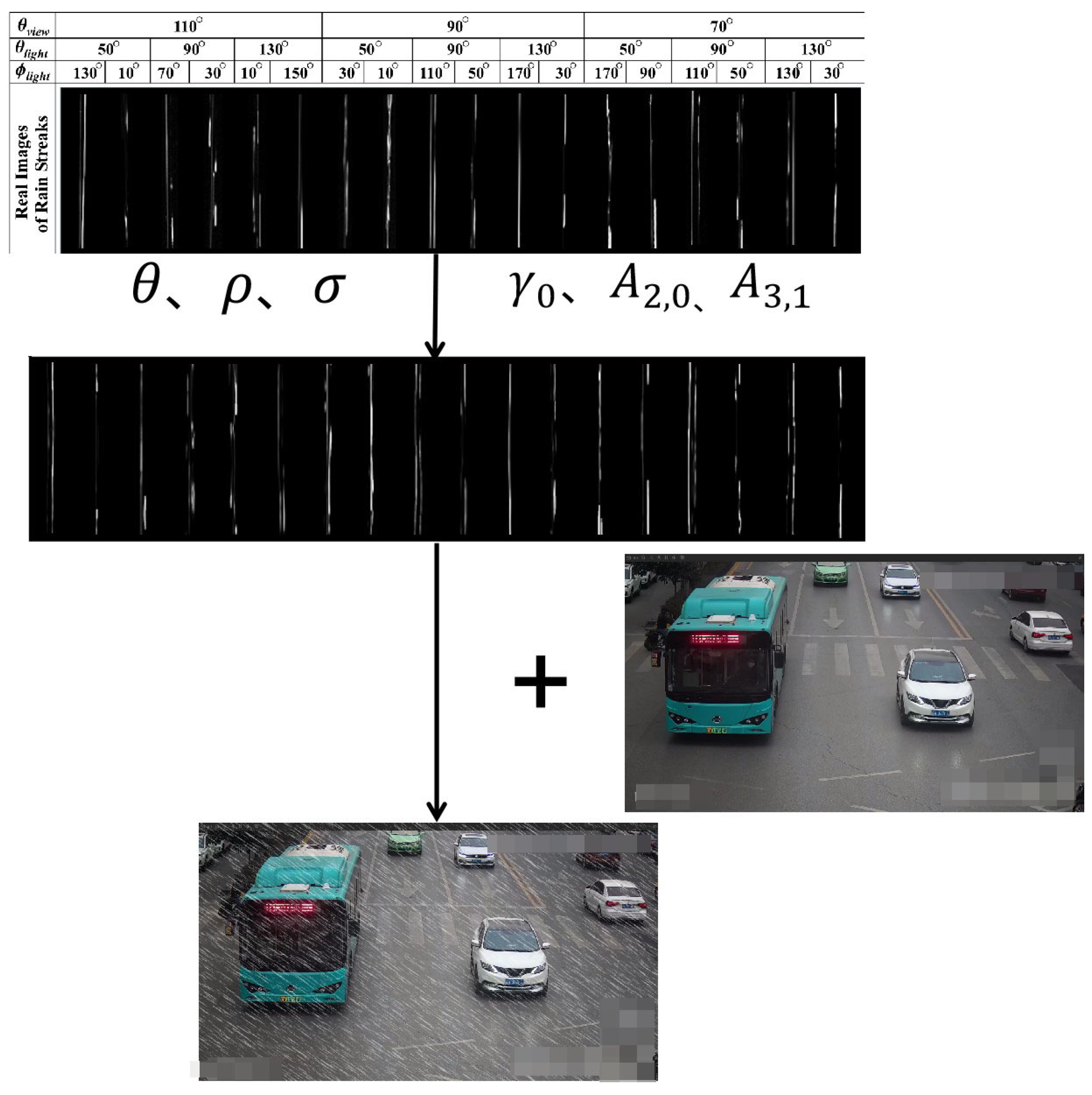
- (1)
- First, the rain-streak patterns under the conditions of two light sources with different angles of illumination and different camera directions are constructed.
- (2)
- Then, the rain images are synthesized according to the raindrop-modeling equation:where r is the surface tension, is the density of water, is the angle, is the azimuth, is the size of the raindrop, and are the amplitudes, and is the frequency, is the Legendre function that describes the dependence of the shape on the angle for the mode (n,m). The parameters are usually set by empirical knowledge ( and , 2006 [29]), and the rain pattern is synthesized by formulas and .
- (3)
- Finally, the synthesized rain pattern is directly added to the clean background image to get the rain image.
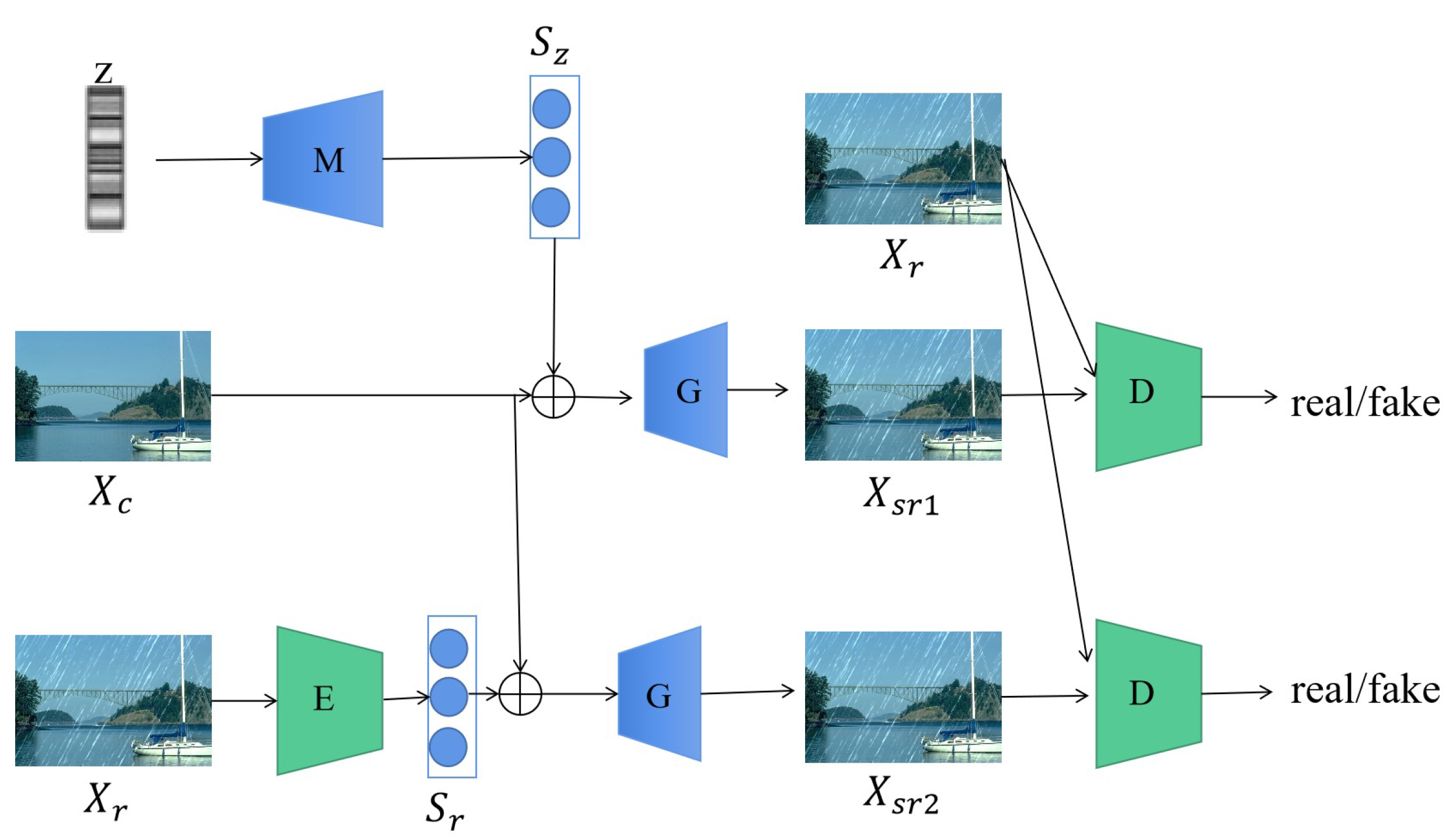
2.2. Data-Driven Rain-Image-Rendering Technology
2.3. Single-Image Rain-Removal Algorithm
2.4. Vehicle-Color Recognition Algorithms
3. Construction of -24
3.1. -24
3.2. Rendering by
3.3. Rendering by the Algorithm
4. Experimental Results
4.1. Experimental Setup
4.2. Model Trained on and -24
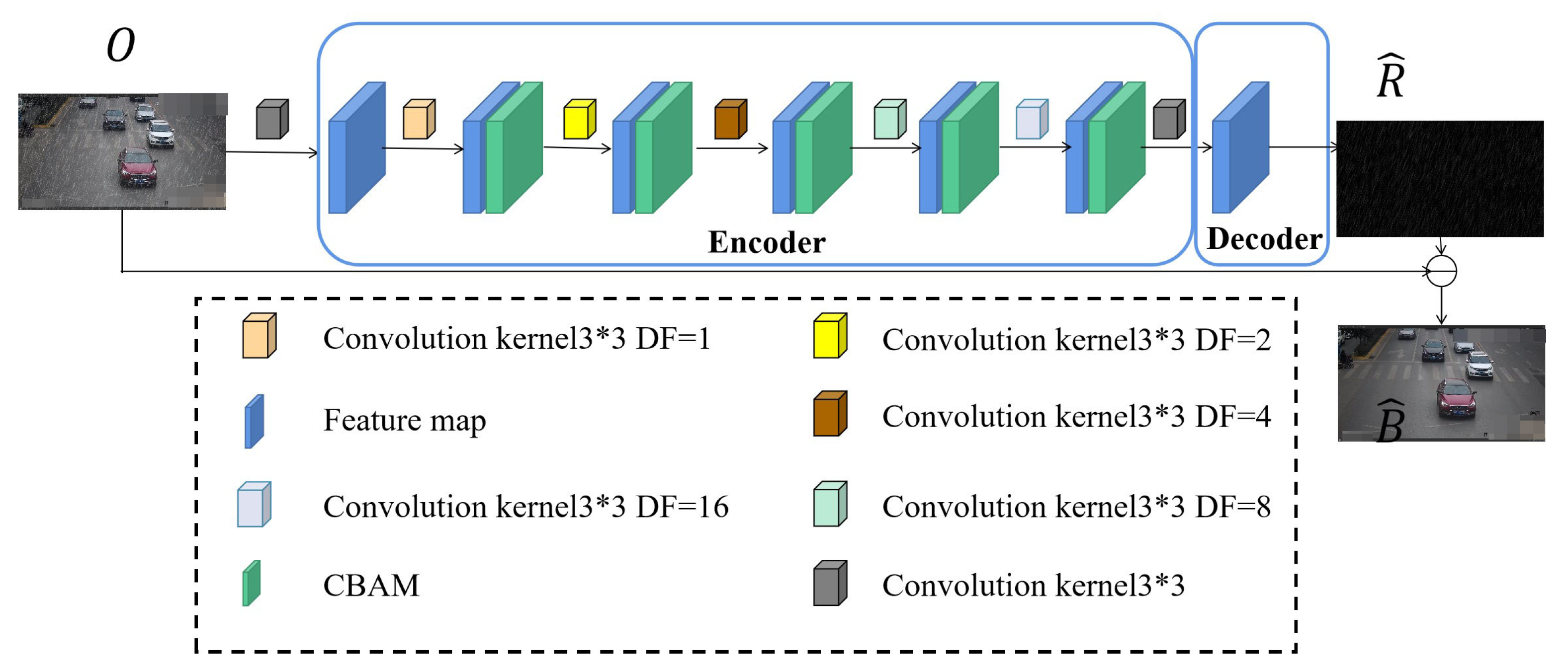
4.2.1. Network
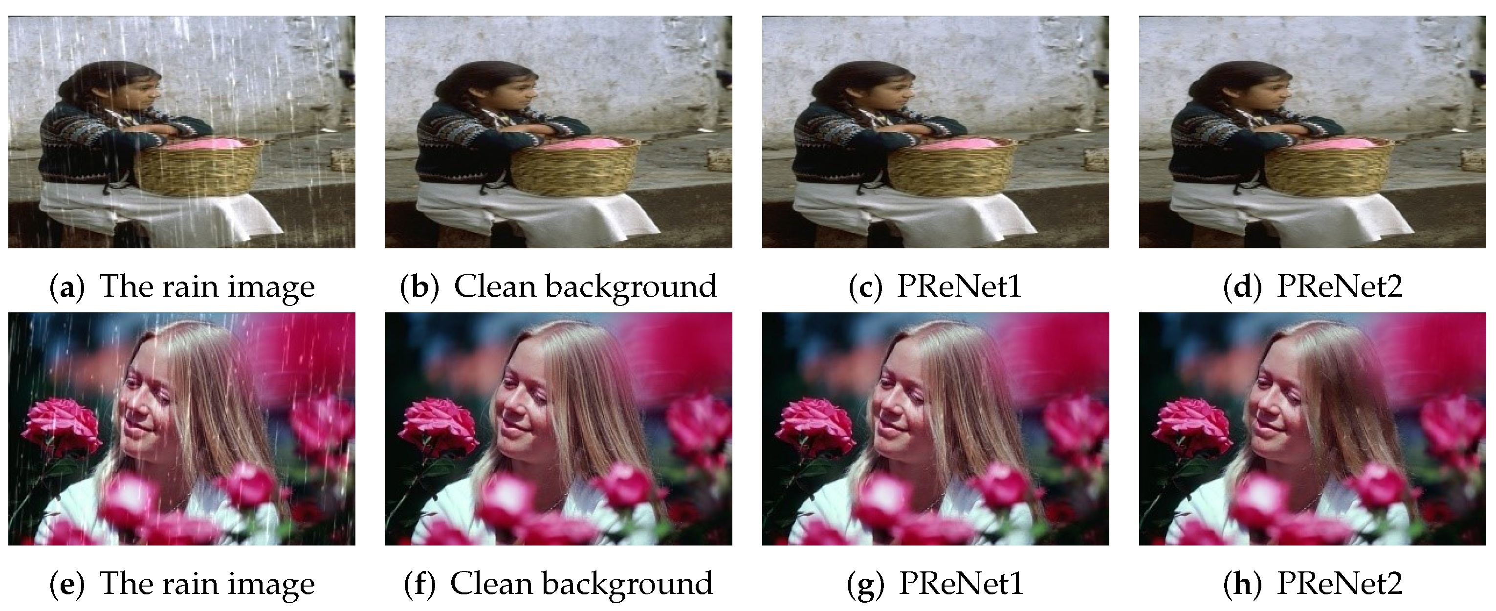
4.2.2. Comparison of Synthetic Rain Images
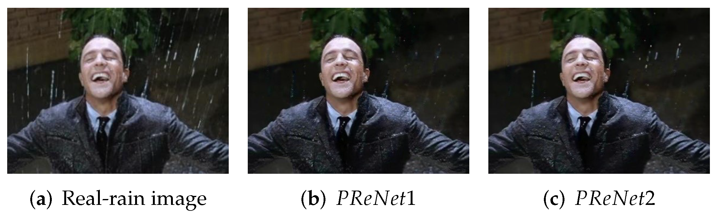
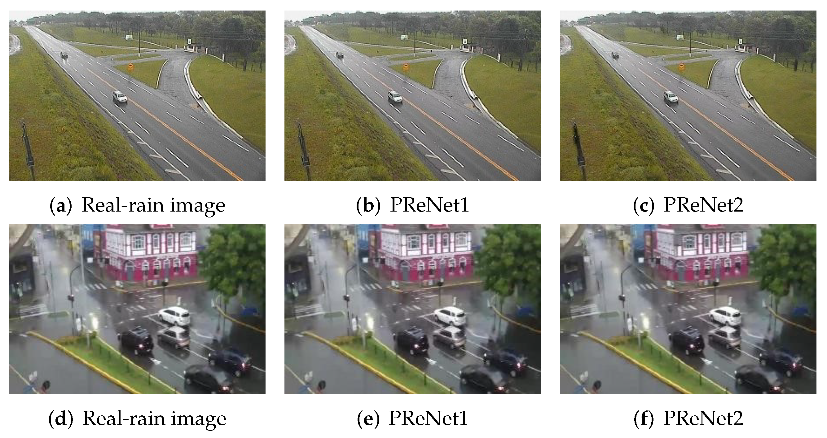
4.2.3. Comparison of Real Rain Images
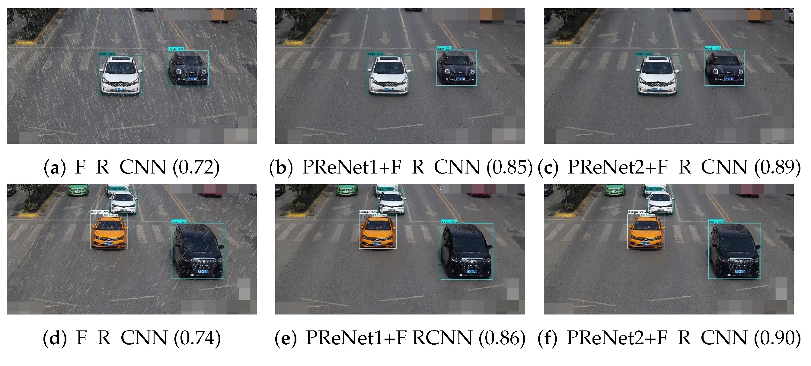
4.2.4. Comparison of Recognition Effects of Low- and High-Level Joint Tasks
4.3. Model Tested on and -24
4.3.1. Network
4.3.2. Comparison on Synthetic Rain Image
4.3.3. Comparison of Real Rain Images
4.4. Object Detection Models Trained by -24 and -24
5. Conclusions
Author Contributions
Funding
Institutional Review Board Statement
Informed Consent Statement
Data Availability Statement
Conflicts of Interest
References
- Chen, P.; Bai, X.; Liu, W. Vehicle color recognition on urban road by feature context. IEEE Trans. Intell. Transp. Syst. 2014, 15, 2340–2346. [Google Scholar]
- Tariq, A.; Khan, M.Z.; Khan, M.U.G. Real Time Vehicle Detection and Colour Recognition using tuned Features of Faster-RCNN. In Proceedings of the 2021 1st International Conference on Artificial Intelligence and Data Analytics (CAIDA), Riyadh, Saudi Arabia, 6–7 April 2021; pp. 262–267. [Google Scholar]
- Jeong, Y.; Park, K.H.; Park, D. Homogeneity patch search method for voting-based efficient vehicle color classification using front-of-vehicle image. Multimed. Tools Appl. 2019, 78, 28633–28648. [Google Scholar]
- Hu, M.; Bai, L.; Li, Y.; Zhao, S.R.; Chen, E.H. Vehicle 24-Color Long Tail Recognition Based on Smooth Modulation Neural Network with Multi-layer Feature Representation. arXiv 2021, arXiv:2107.09944. [Google Scholar]
- Hu, M.; Wu, Y.; Song, Y.; Yang, J.; Zhang, R.; Wang, H.; Meng, D. The integrated evaluation and review of single image rain removal based. J. Image Graph. 2022, 10, 11834. [Google Scholar]
- Xu, C.D.; Zhao, X.R.; Jin, X.; Wei, X.S. Exploring categorical regularization for domain adaptive object detection. In Proceedings of the IEEE/CVF Conference on Computer Vision and Pattern Recognition, Seattle, WA, USA, 13–19 June 2020; pp. 11724–11733. [Google Scholar]
- Vs, V.; Gupta, V.; Oza, P.; Sindagi, V.A.; Patel, V.M. Mega-cda: Memory guided attention for category-aware unsupervised domain adaptive object detection. In Proceedings of the IEEE/CVF Conference on Computer Vision and Pattern Recognition, Nashville, TN, USA, 20–25 June 2021; pp. 4516–4526. [Google Scholar]
- Xu, M.; Wang, H.; Ni, B.; Tian, Q.; Zhang, W. Cross-domain detection via graph-induced prototype alignment. In Proceedings of the IEEE/CVF Conference on Computer Vision and Pattern Recognition, Seattle, WA, USA, 13–19 June 2020; pp. 12355–12364. [Google Scholar]
- Zhang, Y.; Wang, Z.; Mao, Y. Rpn prototype alignment for domain adaptive object detector. In Proceedings of the IEEE/CVF Conference on Computer Vision and Pattern Recognition, Nashville, TN, USA, 20–25 June 2021; pp. 12425–12434. [Google Scholar]
- Li, W.; Liu, X.; Yuan, Y. SIGMA: Semantic-complete Graph Matching for Domain Adaptive Object Detection. In Proceedings of the IEEE/CVF Conference on Computer Vision and Pattern Recognition, New Orleans, LA, USA, 19–23 June 2022; pp. 5291–5300. [Google Scholar]
- Shan, Y.; Lu, W.F.; Chew, C.M. Pixel and feature level based domain adaptation for object detection in autonomous driving. Neurocomputing 2019, 367, 31–38. [Google Scholar]
- Tilakaratna, D.S.; Watchareeruetai, U.; Siddhichai, S.; Natcharapinchai, N. Image analysis algorithms for vehicle color recognition. In Proceedings of the 2017 International Electrical Engineering Congress (iEECON), Pattaya, Thailand, 8–10 March 2017; pp. 1–4. [Google Scholar]
- Kim, T.; Jeong, M.; Kim, S.; Choi, S.; Kim, C. Diversify and match: A domain adaptive representation learning paradigm for object detection. In Proceedings of the IEEE/CVF Conference on Computer Vision and Pattern Recognition, Long Beach, CA, USA, 15–20 June 2019; pp. 12456–12465. [Google Scholar]
- Dong, H.; Pan, J.; Xiang, L.; Hu, Z.; Zhang, X.; Wang, F.; Yang, M.H. Multi-scale boosted dehazing network with dense feature fusion. In Proceedings of the IEEE/CVF Conference on Computer Vision and Pattern Recognition, Seattle, WA, USA, 13–19 June 2020; pp. 2157–2167. [Google Scholar]
- Sindagi, V.A.; Oza, P.; Yasarla, R.; Patel, V.M. Prior-based domain adaptive object detection for hazy and rainy conditions. In European Conference on Computer Vision; Springer: Berlin/Heidelberg, Germany, 2020; pp. 763–780. [Google Scholar]
- Wang, T.; Zhang, X.; Yuan, L.; Feng, J. Few-shot adaptive faster r-cnn. In Proceedings of the IEEE/CVF Conference on Computer Vision and Pattern Recognition, Long Beach, CA, USA, 15–20 June 2019; pp. 7173–7182. [Google Scholar]
- Li, Y.; Tan, R.T.; Guo, X.; Lu, J.; Brown, M.S. Rain streak removal using layer priors. In Proceedings of the IEEE Conference on Computer Vision and Pattern Recognition, Las Vegas, NV, USA, 27–30 June 2016; pp. 2736–2744. [Google Scholar]
- Yang, W.; Tan, R.T.; Feng, J.; Liu, J.; Guo, Z.; Yan, S. Deep joint rain detection and removal from a single image. In Proceedings of the IEEE Conference on Computer Vision and Pattern Recognition, Honolulu, HI, USA, 21–26 July 2017; pp. 1357–1366. [Google Scholar]
- Hu, X.; Fu, C.W.; Zhu, L.; Heng, P.A. Depth-attentional features for single-image rain removal. In Proceedings of the IEEE/CVF Conference on Computer Vision and Pattern Recognition, Long Beach, CA, USA, 15–20 June 2019; pp. 8022–8031. [Google Scholar]
- Tremblay, M.; Halder, S.S.; De Charette, R.; Lalonde, J.F. Rain rendering for evaluating and improving robustness to bad weather. Int. J. Comput. Vis. 2021, 129, 341–360. [Google Scholar]
- Wei, Y.; Zhang, Z.; Wang, Y.; Xu, M.; Yang, Y.; Yan, S.; Wang, M. Deraincyclegan: Rain attentive cyclegan for single image deraining and rainmaking. IEEE Trans. Image Process. 2021, 30, 4788–4801. [Google Scholar]
- Wang, H.; Yue, Z.; Xie, Q.; Zhao, Q.; Zheng, Y.; Meng, D. From rain generation to rain removal. In Proceedings of the IEEE/CVF Conference on Computer Vision and Pattern Recognition, Nashville, TN, USA, 20–25 June 2021; pp. 14791–14801. [Google Scholar]
- Wang, T.; Yang, X.; Xu, K.; Chen, S.; Zhang, Q.; Lau, R.W. Spatial attentive single-image deraining with a high quality real rain dataset. In Proceedings of the IEEE/CVF Conference on Computer Vision and Pattern Recognition, Long Beach, CA, USA, 15–20 June 2019; pp. 12270–12279. [Google Scholar]
- Choi, J.; Kim, D.H.; Lee, S.; Lee, S.H.; Song, B.C. Synthesized rain images for deraining algorithms. Neurocomputing 2022, 492, 421–439. [Google Scholar]
- Ren, D.; Zuo, W.; Hu, Q.; Zhu, P.; Meng, D. Progressive image deraining networks: A better and simpler baseline. In Proceedings of the IEEE/CVF Conference on Computer Vision and Pattern Recognition, Long Beach, CA, USA, 15–20 June 2019; pp. 3937–3946. [Google Scholar]
- Hu, M.; Yang, J.; Ling, N.; Liu, Y.; Fan, J. Lightweight single image deraining algorithm incorporating visual saliency. IET Image Process. 2022, 16, 3190–3200. [Google Scholar]
- Li, S.; Ren, W.; Zhang, J.; Yu, J.; Guo, X. Single image rain removal via a deep decomposition–composition network. Comput. Vis. Image Underst. 2019, 186, 48–57. [Google Scholar]
- Wang, Y.; Ma, C.; Zeng, B. Multi-decoding deraining network and quasi-sparsity based training. In Proceedings of the IEEE/CVF Conference on Computer Vision and Pattern Recognition, Nashville, TN, USA, 20–25 June 2021; pp. 13375–13384. [Google Scholar]
- Garg, K.; Nayar, S.K. Photorealistic rendering of rain streaks. ACM Trans. Graph. 2006, 26, 996–1002. [Google Scholar]
- Qian, R.; Tan, R.T.; Yang, W.; Su, J.; Liu, J. Attentive generative adversarial network for raindrop removal from a single image. In Proceedings of the IEEE Conference on Computer Vision and Pattern Recognition, Salt Lake City, UT, USA, 18–23 June 2018; pp. 2482–2491. [Google Scholar]
- Jin, J.; Fatemi, A.; Lira, W.M.P.; Yu, F.; Leng, B.; Ma, R.; Mahdavi-Amiri, A.; Zhang, H. Raidar: A rich annotated image dataset of rainy street scenes. In Proceedings of the IEEE/CVF International Conference on Computer Vision, Montreal, BC, Canada, 11–17 October 2021; pp. 2951–2961. [Google Scholar]
- Chen, D.Y.; Chen, C.C.; Kang, L.W. Visual depth guided color image rain streaks removal using sparse coding. IEEE Trans. Circuits Syst. Video Technol. 2014, 24, 1430–1455. [Google Scholar]
- Luo, Y.; Xu, Y.; Ji, H. Removing rain from a single image via discriminative sparse coding. In Proceedings of the IEEE International Conference on Computer Vision, Santiago, Chile, 7–13 December 2015; pp. 3397–3405. [Google Scholar]
- Fu, X.; Huang, J.; Ding, X.; Liao, Y.; Paisley, J. Clearing the skies: A deep network architecture for single-image rain removal. IEEE Trans. Image Process. 2017, 26, 2944–2956. [Google Scholar]
- Fu, X.; Liang, B.; Huang, Y.; Ding, X.; Paisley, J. Lightweight pyramid networks for image deraining. IEEE Trans. Neural Netw. Learn. Syst. 2019, 31, 1794–1807. [Google Scholar] [PubMed]
- Xue, P.; He, H. Research of Single Image Rain Removal Algorithm Based on LBP-CGAN Rain Generation Method. Math. Probl. Eng. 2021, 2021, 8865843. [Google Scholar]
- Wang, H.; Xie, Q.; Wu, Y.; Zhao, Q.; Meng, D. Single image rain streaks removal: A review and an exploration. Int. J. Mach. Learn. Cybern. 2020, 11, 853–872. [Google Scholar]
- Ren, S.; He, K.; Girshick, R.; Sun, J. Faster r-cnn: Towards real-time object detection with region proposal networks. Adv. Neural Inf. Process. Syst. 2015, 28. [Google Scholar]
- Zhang, X.; Wang, J.; Zhan, J.; Dai, J. Fuzzy measures and Choquet integrals based on fuzzy covering rough sets. IEEE Trans. Fuzzy Syst. 2021, 30, 2360–2374. [Google Scholar]
- Sheng, N.; Zhang, X. Regular partial residuated lattices and their filters. Mathematics 2022, 10, 2429. [Google Scholar] [CrossRef]
- Wang, J.; Zhang, X. A novel multi-criteria decision-making method based on rough sets and fuzzy measures. Axioms 2022, 11, 275. [Google Scholar] [CrossRef]
- Liang, R.; Zhang, X. Interval-valued pseudo overlap functions and application. Axioms 2022, 11, 216. [Google Scholar] [CrossRef]


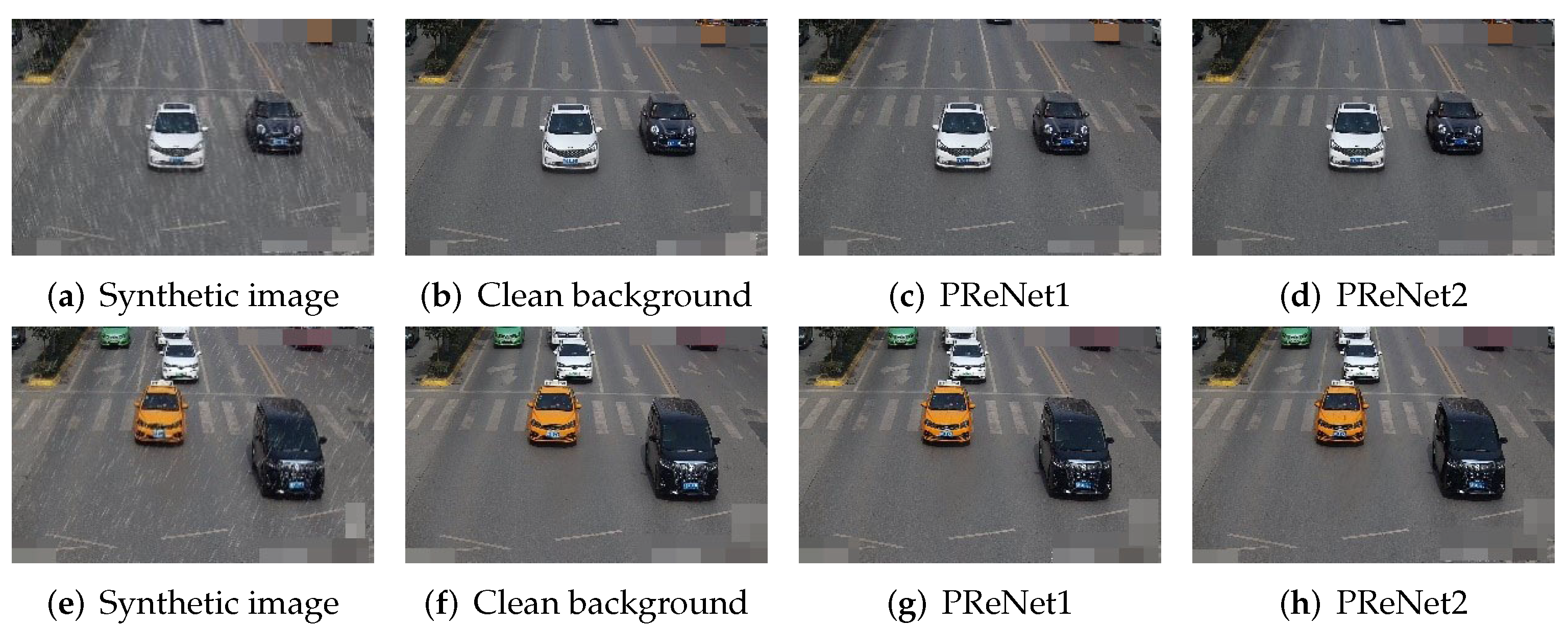
| Metrics | Models | PReNet1 | PReNet2 | ||
|---|---|---|---|---|---|
| Datasets | |||||
| Rain100L | PSNR | SSIM | PSNR | SSIM | |
| 32.67 | 0.965 | 32.44 | 0.945 | ||
| Rain Vehicle Color-24 | PSNR | SSIM | PSNR | SSIM | |
| 31.62 | 0.955 | 33.51 | 0.973 | ||
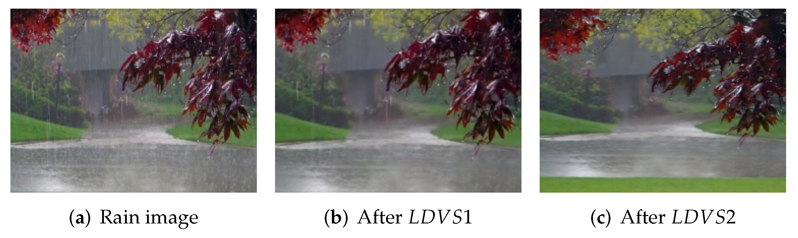
| Metrics | Models | LDVS1 | LDVS2 | ||
|---|---|---|---|---|---|
| Datasets | |||||
| Rain100L | PSNR | SSIM | PSNR | SSIM | |
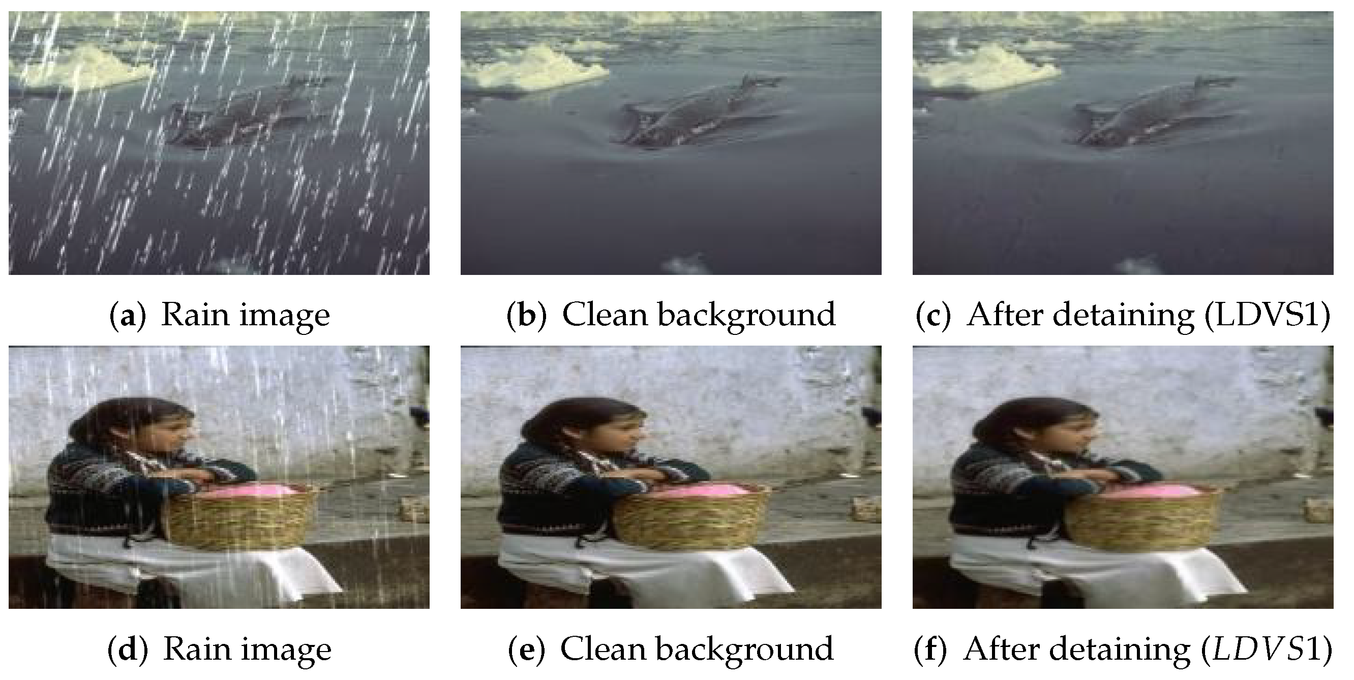
| 33.56 | 0.959 | 33.12 | 0.960 | ||
| Rain Vehicle Color-24 | PSNR | SSIM | PSNR | SSIM | |
| 31.23 | 0.951 | 34.34 | 0.960 | ||
| Category | ||||||
|---|---|---|---|---|---|---|
| VC-24 | RVC-24 | VC-24 | RVC-24 | VC-24 | RVC-24 | |
| White | 0.98 | 0.64 | 0.84 | 0.80 | 0.96 | 0.74 |
| Black | 0.97 | 0.52 | 0.82 | 0.31 | 0.95 | 0.38 |
| Orange | 0.98 | 0.85 | 0.81 | 0.71 | 0.96 | 0.81 |
| Silver gray | 0.96 | 0.30 | 0.77 | 0.44 | 0.91 | 0.86 |
| Grass green | 0.98 | 0.82 | 0.70 | 0.61 | 0.96 | 0.96 |
| Dark gray | 0.94 | 0.30 | 0.66 | 0.17 | 0.84 | 0.29 |
| Dark red | 0.98 | 0.63 | 0.78 | 0.24 | 0.93 | 0.44 |
| Gray | 0.89 | 0.06 | 0.18 | 0.13 | 0.54 | 0.13 |
| Red | 0.96 | 0.65 | 0.60 | 0.20 | 0.88 | 0.41 |
| Cyan | 0.97 | 0.82 | 0.75 | 0.33 | 0.92 | 0.46 |
| Champagne | 0.97 | 0.17 | 0.63 | 0.29 | 0.81 | 0.25 |
| Dark blue | 0.96 | 0.39 | 0.66 | 0.12 | 0.86 | 0.36 |
| Blue | 0.97 | 0.59 | 0.73 | 0.10 | 0.87 | 0.69 |
| Dark brown | 0.97 | 0.09 | 0.45 | 0.02 | 0.71 | 0.11 |
| Brown | 0.88 | 0.36 | 0.30 | 0.13 | 0.58 | 0.27 |
| Yellow | 0.97 | 0.66 | 0.51 | 0.13 | 0.79 | 0.18 |
| Lemon yellow | 0.99 | 0.88 | 0.87 | 0.84 | 0.93 | 0.70 |
| Dark orange | 0.96 | 0.67 | 0.65 | 0.18 | 0.78 | 0.13 |
| Dark green | 0.94 | 0.28 | 0.38 | 0.08 | 0.58 | 0.00 |
| Red orange | 0.99 | 0.33 | 0.24 | 0.00 | 0.61 | 0.00 |
| Earthy yellow | 0.97 | 0.50 | 0.62 | 0.50 | 0.74 | 0.10 |
| Green | 0.93 | 0.13 | 0.61 | 0.33 | 0.74 | 0.00 |
| Pink | 0.94 | 0.66 | 0.50 | 0.33 | 0.71 | 0.17 |
| Purple | 0.80 | 0.00 | 0.00 | 0.00 | 0.19 | 0.00 |
| mAP | 94.96% | 47.22% | 58.59% | 29.19% | 78.13% | 30.23% |
| Category | ||||||
|---|---|---|---|---|---|---|
| VC-24 | RVC-24 | VC-24 | RVC-24 | VC-24 | RVC-24 | |
| White | 0.62 | 0.60 | 0.94 | 0.96 | 0.94 | 0.95 |
| Black | 0.61 | 0.69 | 0.82 | 0.69 | 0.92 | 0.93 |
| Orange | 0.69 | 0.77 | 0.92 | 0.90 | 0.95 | 0.95 |
| Silver gray | 0.48 | 0.31 | 0.44 | 0.81 | 0.85 | 0.86 |
| Grass green | 0.60 | 0.82 | 0.88 | 0.93 | 0.94 | 0.96 |
| Dark gray | 0.47 | 0.43 | 0.57 | 0.69 | 0.71 | 0.67 |
| Dark red | 0.36 | 0.48 | 0.73 | 0.79 | 0.83 | 0.88 |
| Gray | 0.18 | 0.31 | 0.12 | 0.41 | 0.35 | 0.31 |
| Red | 0.37 | 0.44 | 0.62 | 0.56 | 0.79 | 0.76 |
| Cyan | 0.42 | 0.62 | 0.71 | 0.82 | 0.87 | 0.87 |
| Champagne | 0.33 | 0.28 | 0.46 | 0.74 | 0.65 | 0.73 |
| Dark blue | 0.60 | 0.52 | 0.66 | 0.79 | 0.78 | 0.75 |
| Blue | 0.29 | 0.56 | 0.44 | 0.69 | 0.87 | 0.69 |
| Dark brown | 0.38 | 0.35 | 0.45 | 0.18 | 0.60 | 0.47 |
| Brown | 0.47 | 0.35 | 0.34 | 0.10 | 0.33 | 0.34 |
| Yellow | 0.51 | 0.35 | 0.94 | 0.83 | 0.72 | 0.92 |
| Lemon yellow | 0.32 | 0.57 | 0.95 | 0.99 | 1.00 | 0.75 |
| Dark orange | 0.41 | 0.32 | 0.52 | 0.28 | 0.11 | 0.47 |
| Dark green | 0.62 | 0.59 | 0.10 | 0.18 | 0.36 | 0.34 |
| Red orange | 0.52 | 0.38 | 0.66 | 0.07 | 0.29 | 0.52 |
| Earthy yellow | 1.00 | 0.68 | 0.23 | 0.45 | 0.78 | 0.28 |
| Green | 0.59 | 0.18 | 0.47 | 0.85 | 0.55 | 0.97 |
| Pink | 0.03 | 0.84 | 0.02 | 0.54 | 1.00 | 0.52 |
| Purple | 0.99 | 0.22 | 0.07 | 0.03 | 0.00 | 0.06 |
| mAP | 49.14% | 48.58% | 55.13% | 60.65% | 70.84% | 66.33% |
Publisher’s Note: MDPI stays neutral with regard to jurisdictional claims in published maps and institutional affiliations. |
© 2022 by the authors. Licensee MDPI, Basel, Switzerland. This article is an open access article distributed under the terms and conditions of the Creative Commons Attribution (CC BY) license (https://creativecommons.org/licenses/by/4.0/).
Share and Cite
Hu, M.; Wang, C.; Yang, J.; Wu, Y.; Fan, J.; Jing, B. Rain Rendering and Construction of Rain Vehicle Color-24 Dataset. Mathematics 2022, 10, 3210. https://doi.org/10.3390/math10173210
Hu M, Wang C, Yang J, Wu Y, Fan J, Jing B. Rain Rendering and Construction of Rain Vehicle Color-24 Dataset. Mathematics. 2022; 10(17):3210. https://doi.org/10.3390/math10173210
Chicago/Turabian StyleHu, Mingdi, Chenrui Wang, Jingbing Yang, Yi Wu, Jiulun Fan, and Bingyi Jing. 2022. "Rain Rendering and Construction of Rain Vehicle Color-24 Dataset" Mathematics 10, no. 17: 3210. https://doi.org/10.3390/math10173210
APA StyleHu, M., Wang, C., Yang, J., Wu, Y., Fan, J., & Jing, B. (2022). Rain Rendering and Construction of Rain Vehicle Color-24 Dataset. Mathematics, 10(17), 3210. https://doi.org/10.3390/math10173210