Research on b Value Estimation Based on Apparent Amplitude-Frequency Distribution in Rock Acoustic Emission Tests

Abstract

The rock acoustic emission (AE) technique has often been used to study rock destruction properties and has also been considered an important measure for simulating earthquake foreshock sequences. Among them, the AE b value is an essential parameter for the size distribution characteristics and probabilistic hazard analysis of rock fractures. Variations in b values obtained in rock AE tests and earthquakes are often compared to establish analogies in the damage process and precursory analysis. Nevertheless, because the amplitudes measured on the sample boundary by an acoustic sensor (apparent amplitude) are often used to estimate the b value, which cannot descript the source size distribution, it is necessary to develop a method to obtain the size distribution characteristics of the real source from the apparent amplitude in doubly truncated distribution. In this study, we obtain AE apparent amplitudes by applying an attenuation operator to source amplitudes generated by a computer with an underlying exponential distribution and then use these simulated apparent amplitudes to perform a comparative analysis of various b value estimation methods that are used in earthquakes and propose an optimal b value estimation procedure for rock AE tests through apparent amplitudes. To further verify the reliability of the newly proposed procedure, a b value characteristics analysis was carried out on a non-explosive expansion agent rock AE test and transparent refractive index experiment with red sandstone, marble, granite, and limestone. The results indicate that mineral grains of different sizes and compositions and different types of discontinuities of rock specimens determine the rock fracture characteristics, as well as the b value. The dynamic b values decreased linearly during the loading process, which confirms that variations in the b value also depend on the stress. These results indicate that the newly proposed procedure for estimating the b value in rock AE tests based on apparent amplitudes has high reliability.

1. Introduction

The power law size distribution relationship of source energy E or seismic moment M₀ is an intrinsic characteristic of the frequency-size distribution in statistical seismology; it can well record the spatial and temporal distribution of rock fractures from a large number of small-scale ruptures to fewer large-scale ruptures, and it has been widely used in seismic research. Since there is a logarithmic relationship between the local magnitude M and the source energy E or seismic moment M₀, we can conclude that the local magnitude-frequency distribution obeys the exponential Gutenberg–Richter (G–R) law [1], which has also been widely used for probabilistic seismic hazard analysis [2,3,4,5,6,7]. The G–R law is expressed on a logarithmic scale given by

$${\log }_{10}(N)=a-bM$$

(1)

where a and b are constants and N is the number of earthquakes that occur in a specific time window with magnitude ≥ M. More importantly, parameter a reflects the size of the time window of observation; slope b is an essential tool in seismotectonic studies and seismic-risk analysis within the same time window in a certain area [5,8], which is often referred to as the b value. More recently, the b value in the G–R law has also been interpreted as an indicator of the applied shear stress and material heterogeneity [9,10,11,12,13,14]. Thus, its correct computation represents an important challenge in seismology and rock mechanics [15,16,17,18].

The selected discontinuities and missing earthquake events in the magnitude-frequency distribution are the main effects on stable b value estimation, which is why the two ends of the magnitude-frequency distribution deviate from the G–R law. For some authors, the right and left end points deviating from the G–R law correspond to the magnitude of completeness M_c (which is defined as the lowest magnitude at which 100% of the events in a space–time volume are detected [8,19] and the auxiliary magnitude M₀, respectively. Many different procedures for correctly estimating M_c and M₀ have been proposed [8,19,20,21,22,23,24,25]. Figure 1 shows that with the value of the assumed M_c starting from the minimum magnitude in the catalog and increasing gradually, the corresponding b value and goodness-of-fit change significantly as M_c ≤ 2 and tend to be stable as M_c ≥ 2. In view of this phenomenon, some researchers hope to select a sufficiently large M_c to estimate the b value, but for the statistical value of M_c and b, which will reduce a large number of low-magnitude events and further lead to a decrease in the space–time resolution of variations in M_c and reliability and robustness of the b value estimation [26,27]. Therefore, accurately determining M_c has become the key to stably estimating the b values.

In rock mechanics, the acoustic emission (AE) technique is often used to study the destruction properties of rocks by recording elastic wave information radiated by crack initiation, propagation, and penetration during rock deformation [28,29,30,31]. Additionally, the AE test method is also an important means to simulate earthquake foreshock sequences and study focal mechanisms [14,32,33,34,35,36,37,38,39,40,41,42]. Therefore, the space–time variation characteristics of the b value obtained in rock AE deformation tests have been used to simulate earthquake precursor characteristics [43,44,45,46,47]. However, unlike the magnitude used in Equation (1) for b value estimation in seismology, AE equipment records the high-frequency elastic wave signal of the small-scale rupture, and the AE amplitude is the apparent amplitude measured by sensors at the sample boundary after attenuation from the seismic source [25]. The corresponding apparent amplitude-frequency distribution does not represent the source size distribution. Thus, the frequency-size distribution law of the source signals collected by the sensors in the rock AE test will be changed owing to the elastic wave attenuation, and the same deviation will appear at both ends of the amplitude-frequency as the magnitude-frequency distribution [33,37], which would affect the size of the real b value. (Here, the analogy with the earthquake is used to define the left and right deviation points of the amplitude-frequency distribution of the rock AE test as the completeness amplitude point A_c and auxiliary discontinuous amplitude point A₀, respectively.) Although some researchers have long been concerned about the influence of attenuation on the amplitude-frequency distribution in rock AE tests and have also proposed some corresponding compensation methods to obtain the equivalent AE magnitude with the same significance as the magnitude of the earthquake to analyze rock b value characteristics [44,48], the equivalent amplitude distribution still cannot fully represent the real frequency-size distribution of rock cracks. To solve this problem, Liu [25] used a statistical method to prove that the apparent amplitude-frequency distribution retains the source frequency-size distribution characteristics, wherein the key to estimating the real b value is to properly truncate the apparent amplitude-frequency distribution. A new b value estimation method called the Fisher optimal split and global search algorithm (FGS) was proposed to identify the log-linear segment from the apparent amplitude-frequency distribution of the rock AE test for b value estimation. In addition, because AE acquisition equipment is very sensitive to the interference of test conditions, such as environmental noise and current signals, a high threshold value of the signal acquisition is generally set for laboratory rock AE tests. Thus, the completeness amplitude A_c is usually ignored. Therefore, the completeness of the amplitude data should also be considered when considering how to obtain the source size distribution characteristic parameters using the apparent amplitude-frequency distribution in the estimation of the rock AE b value.

Based on the discussion above, firstly, we carried out a synthetic AE simulation test to compare and analyze the applicability of the completeness magnitude estimation methods commonly used in earthquakes for the estimation of rock AE completeness amplitude and proposed an optimal procedure for rock AE b value estimation by combining Bootstrap [8] and the FGS method which is used for estimating the characteristic parameters of the source size distribution from the apparent amplitude-frequency distribution. Then, we designed a static dilation rock rupturing AE test to further verify the reliability of the newly proposed optimal procedure of b value estimation based on the relationship between the b value and rock microscopic composition and stress to provide a reliable and accurate b value estimation procedure for laboratory rock AE tests. As a result, this research can provide new insights and methods in the analysis of the precursory characteristics in laboratory rock AE tests and rock mass engineering.

2. Optimal b Value Estimation Procedure Based on Apparent Amplitude-Frequency Distribution

In rock AE tests, a high threshold is generally set to remove noise interference, and AE equipment will also define the upper limit amplitude, which will result in a doubly truncated distribution of apparent amplitude frequency, so the completeness amplitude A_c in the b value estimation is usually ignored. In this section, generate AE synthetic data with apparent amplitude and select the estimation method of completeness magnitude M_c commonly used in seismic research to obtain an optimal algorithm for determining completeness magnitude A_c, which is a key step for b value estimation. Then, combined with the nonparametric statistical Bootstrap method, we compared the obtained optimal algorithm of A_c with the FGS method and determined an optimal procedure of the b value estimated for the apparent amplitude data.

2.1. Synthetic Catalogues of Rock AE Apparent Amplitude

Because the true underlying completeness amplitude A_c and b values are not known in a laboratory rock AE test, we designed a specific simulation scheme to randomly generate synthetic AE data that can be used to clearly compare five A_c estimation methods [8,23,24,25]. According to the previous statistical proof and synthetic data generation method [25,49], we designed to generate data arrays with the same length of source amplitude and amount of attenuation, which are all in decibels with a round-off interval of 1 dB. The apparent amplitude after attenuation can be obtained by the subtraction of two randomly arranged arrays of source amplitude and the amount of attenuation. The specific simulation schemes are as follows: firstly, as the b value of most papers is equal to about 1 [50], we generated a source synthetic catalog of i = 1, 2, …, N events with amplitudes A_i in decibels by randomly sampling an underlying Gutenberg–Richter distribution with b = 1.0666 and std = 8 (standard deviation) which varies between limits A_i^min ≤ A_i ≤ A_i^max and has a probability density function p(A_i). Then, we generated an attenuation amount catalog δA_i also in decibels with the same length of A_i, which varies between limits δA_i^min ≤ δA_i ≤ δA_i^max and has a probability density function p(δA_i) that obeys the Poisson distribution (or other forms including normal, exponential, Gamma, and random uniform distributions). Finally, the catalog obtained by the subtraction of randomly arranged A_i and δA_i was used to model the amplitude observed at the sample boundary A_i^obs = A_i − δA_i. In other words, the interval of the apparent amplitude that still follows the exponential distribution was [A_i^min − δA_i^min, A_i^max − δA_i^max]. In this paper, we set A_i^min = 50 dB, A_i^max = 109 dB, δA_i^min = 1 dB, and A_i^max = 10 dB to make the apparent amplitude range of synthetic data close to that in normal rock AE experiment. As a matter of fact, the selection of the ranges for source amplitude and attenuation generation has no effect on the results [49]. In addition, to minimize the effect of data volume on deviation discussion, a data volume of 100,000 was generated. Figure 2A shows the apparent amplitude-frequency distribution of generated data.

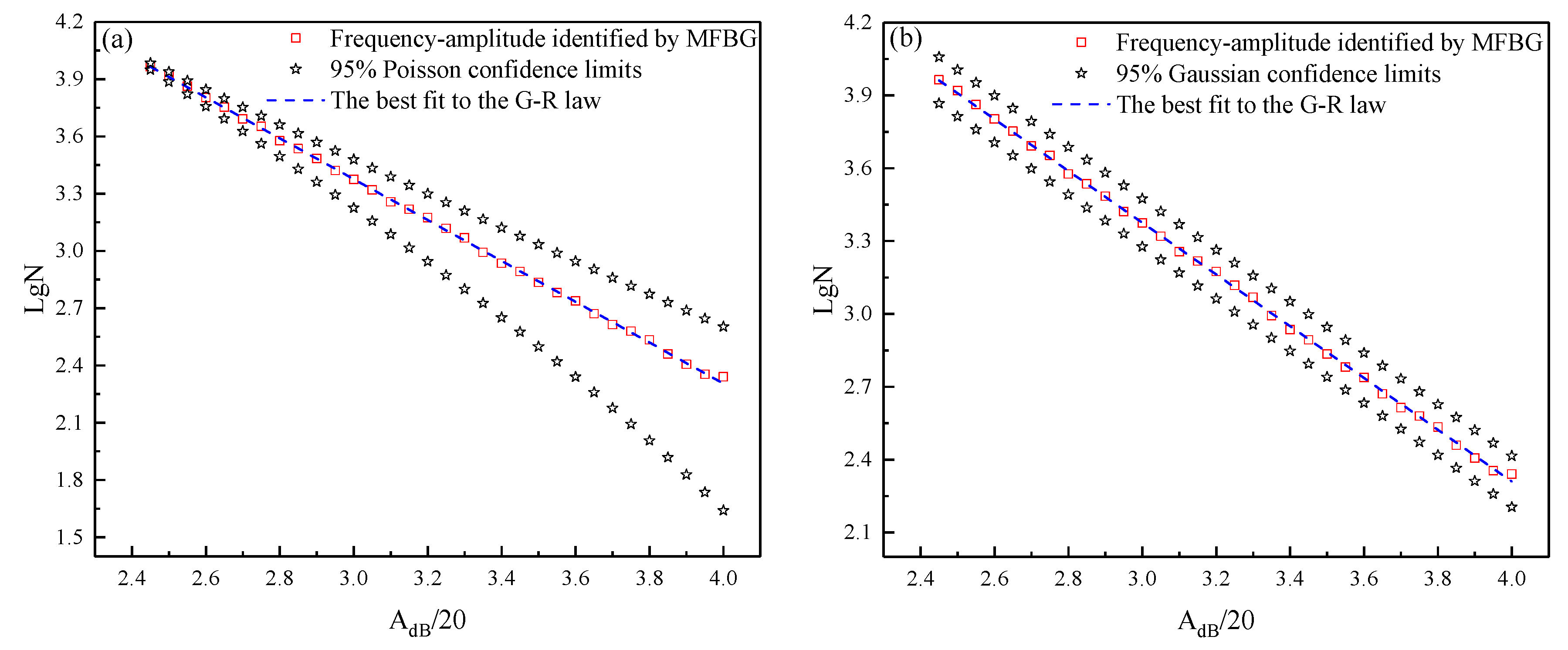
2.2. Determination of Optimal Estimation Method for A_c and A₀

In studies on the earthquake sequence, determining the completeness magnitude M_c is the priority of the seismic sequence analysis. In fact, the core of various seismic b value estimation methods is the algorithm for searching for M_c. As some theories in seismic research are often used in rock AE tests, these M_c estimation methods can also be applied to estimate the completeness amplitude A_c of the rock AE apparent amplitude-frequency distribution. Common M_c estimation methods are as follows:

(1)

Maximum curvature method (MAXC) [23]

(2)

Goodness-of-fit test (GFT) [23]

(3)

M_c by b value stability (MBS) [24]

(4)

Median-based analysis of segment slope (MBASS) [8]

(5)

Fisher optimal split and Global Search algorithm (FGS) [25]

These methods have different algorithms for determining the completeness magnitude M_c. As shown in Figure 2A, the MAXC approach identifies the magnitude corresponding to the maximum curvature of the cumulative magnitude-frequency distribution as M_c. In fact, this point is also the magnitude corresponding to the maximum frequency of the incremental magnitude-frequency distribution. The GFT method in Figure 2B determines M_c by comparing the goodness-of-fit R of the fitted frequency-magnitude distribution with that of the actual magnitude-frequency distribution, and the M_c corresponding to R ≥ 95% confidence is taken as the completeness magnitude (R ≥ 90% confidence can also be accepted as a completeness magnitude in the actual complex earthquake catalog). The MBS method selects the starting point of magnitude where the change in the b value tends to be stable as M_c (Figure 2C), that is:

$$\Delta b=\left|b_{ave}-b\right|\le \delta b$$

(2)

where b_ave is the average estimated b value from each magnitude within the magnitude interval [M_co, M_co + dM] and δb is the uncertainty of the b value proposed by Shi [51]. b_ave and δb can be obtained from Equations (3) and (4):

$$b_{ave}={\displaystyle {\sum }_{M_{co}}^{M_{co}+dM}b(M_{co})}•\frac{\Delta M}{dM}$$

(3)

$$\delta b=2.3b^2\sqrt{\frac{{\displaystyle {\sum }_{i=1}^N{(M_i-\langle M\rangle )}^2}}{N(N-1)}}$$

(4)

where b is the b value of the current magnitude M_co, N is the number of events, M_i is the magnitude corresponding to event N_i, ∆M is the bin width, and <M> is the average magnitude of all events greater than M_co. The FGS method integrates the Fisher optimal split and global search algorithms to determine the log-linear segment of the incremental amplitude-frequency distribution. As shown in Figure 2E, the FGS fully considers the influence of data volume and goodness-of-fit on the estimation results.

Because the b value is a statistical parameter, the b value estimation will be more stable and accurate with the increase in data volume, and this conclusion has already been discussed by many researchers [8,50,52]. Here, we compared the accuracy of b value estimation using synthetic AE amplitude data generated in Section 2.1 to explore the differences in the above five completeness amplitude estimation methods under different data volumes. We randomly generated a source amplitude that obeyed an exponential distribution with a theoretical b value of 1.0666 and a data volume of 100,000 as [50, 109] dB and assumed that the attenuation obeyed the Poisson distribution with the interval of [1, 10] dB. According to the theoretical proof of Liu [25], the amplitude interval that still obeys the exponential distribution after attenuation is [49, 99] dB. Therefore, the theoretical completeness amplitude A_c of the synthetic apparent amplitude data is 2.45. Then, Bootstrap was used to extract 1000 samples from apparent amplitude data with data volumes of 100, 200, 300, 500, 800, 1000, 2000, 3000, 5000, 8000, 10,000, 30,000, 50,000, and 100,000. Figure 3 shows the variation in average A_c and average b value of 1000 Bootstrap samples with different data volumes; the error bar in the figure is the Bootstrap 95% confidence limit.

As shown in Figure 3, the accuracy of A_c estimated by the five methods was positively correlated with the accuracy of the b value, which indicates that selecting an appropriate A_c is very important for the correct b value estimation. This also proves the availability of generated synthetic data to simulate real AE data to a certain degree. It can be seen from the stability of the estimation results that the goodness-of-fit of all methods exceeded 0.9 when the data volume was 3000. Because GFT-90% uses the cumulative amplitude-frequency distribution to estimate A_c, the goodness-of-fit can reach 0.9 just for a data volume of 100. An interesting phenomenon is that the accuracy of the A_c and b values decreased with an increase in the data volume, and only when the data volume was greater than 300, the results of 1000 Bootstrap samples could be successfully searched. MBASS is more dependent on the amount of data and requires at least 5000 data volumes to successfully search the results of 1000 Bootstrap samples. Therefore, these two methods are not suitable for estimating the A_c and b values. The confidence limits and uncertainty of MAXC and MBS were consistent when the data volume was less than 3000. However, when the data volume was greater than 3000, the confidence limits of the MAXC and FGS methods began to gradually decrease to 0, while the mean A_c and b value estimation of MBS exceeded the theoretical value, and the uncertainty of A_c was evident. In addition, because both A_c and b are statistical values, the stability of the statistical results largely depends on the amount of data. To better search the log-linear segment, the doubly truncated amplitude-frequency distribution was accepted by FGS, which fully considers the amplitude distribution characteristics. Therefore, the uncertainty of the Bootstrap confidence limit was higher than that of other methods when the data volume was small. However, it can also be seen that the mean A_c and b values of the Bootstrap samples obtained by FGS were still accurate.

The column distribution of A_c obtained by 1000 Bootstrap samples of various completeness amplitude estimation methods is shown in Figure 4. This shows that MAXC was the most stable and reliable, followed by the FGS method. Although the estimation result of the GFT method also seemed very stable, it clearly underestimated the theoretical A_c, which is inconsistent with the actual situation. Similarly, MBASS not only had unstable results but also overestimated A_c by more than 15% of the samples. The MBS also overestimated A_c and reached more than 10% of the samples when the data volume was 10,000 and 50,000. From the above analysis, it can be seen that the estimation methods of completeness magnitude in seismology are also applicable for completeness amplitude A_c in small-scale rock AE tests, despite some differences in searching ability, accuracy, and stability of estimation results among different methods.

As can be seen from the amplitude-frequency distribution in Figure 2, the rock AE data had an auxiliary discontinuous amplitude point A₀ at the end of the high amplitude segment, which was similar to M₀ in the earthquake sequence. Therefore, when estimating the b value based on the G–R law, the high amplitude data greater than A₀ would inevitably affect the accuracy of the b value estimation. As shown in Figure 2D,E, both the MBASS and FGS can estimate the auxiliary discontinuous point of the magnitude-frequency distribution; therefore, which one is more suitable for estimating the auxiliary discontinuous point is worth further discussing. Figure 5 clearly shows that A₀ estimated by MBASS was smaller than A_c. Therefore, we continued to estimate the third discontinuous point. However, only a few of the third discontinuous points met the requirements at the amplitude of 90 dB. By contrast, the FGS method was able to successfully find both end discontinuities, and the estimation A₀ was very close to the theoretical A₀ at the amplitude of 99 dB. Compared with Figure 5a,b, the log-linear segment of the apparent amplitude-frequency distribution between A_c and A₀ identified by the FGS method was much more stable and reasonable than that of the MBASS method. Therefore, the FGS was more suitable for estimating the auxiliary discontinuous point A₀ at the right end of the apparent amplitude-frequency distribution in the rock AE.

2.3. The Optimal b Value Estimation Procedure through Apparent Amplitude-Frequency Distribution for Rock AE Tests

Because the Bootstrap approach can obtain a reliable estimation and avoid outliers, here, combined with the Bootstrap, we proposed to use MAXC to estimate the completeness amplitude A_c and FGS to estimate the auxiliary discontinuous point A₀, respectively. However, after determining A_c and A₀, another issue worth discussing was which regression method we needed to use to estimate the b value of the apparent amplitude-frequency distribution between A_c and A₀.

Most papers still use least-squares regression (LSR), which assumes that the frequency data errors are Gaussian, to estimate the b value. However, frequencies based on count data have Poisson sampling uncertainties, which cause bias when using LSR for b value estimation. Thus, a generalized linear model (GLM) subject to Poisson error can provide a more accurate fit of count data [45,49,53]. Here, we also used the data generation in Section 2.1 to compare LSR assuming a Gaussian error and GLM assuming a Poisson error with apparent amplitude data between A_c and A₀ at a 95% confidence limit. As shown in Figure 6, the confidence intervals of LSR and GLM indicate significantly different changing trends. The confidence intervals of GLM gradually narrow as the amplitude decreases, and the whole amplitude show a “trumpet” shape. However, the confidence interval of LSR remains parallel from small to large amplitudes, which evidently does not conform to the characteristics of the amplitude-frequency distribution. Maximum likelihood estimation (MLE) is currently one of the most popular methods for estimating the b value [54], and it can be seen from

Table 1. Estimated b values by MFBG when using GLM, LSR, and MLE regression.

Theoretical b Value	Estimating Method	Estimated b Value	Standard Deviation	Bias
1.0666	GLM	1.0705	0.0471	0.0039
	LSR	1.0714	0.0039	0.0048
	MLE	1.0711	0.0233	0.0045

that the standard deviation and bias of the b value obtained by this method are also very small. Therefore, once the apparent amplitude-frequency distribution between A_c and A₀ is determined, the MLE is also a good choice for regression [49]. However, it is worth noting that the MLE does not have an accurate confidence interval of the doubly truncated amplitude-frequency distribution and cannot further analyze the uncertainty of the estimation results. Thus, we chose GLM regression to fit log-linear amplitude of apparent amplitude-frequency between the left end point A_c identified by MAXC and the right end point A₀ identified by FGS, and here we named this b value estimation procedure as MFBG (MAXC-FGS-Bootstrap-GLM).

3. Application of MFBG in b Value Estimation of Rock AE Test

To evaluate the performance of the new b value estimation procedure MFBG, a non-explosive fracturing agent expansion was designed to conduct an AE test on red sandstone, marble, granite, and limestone. The rock broke and formed a specific failure surface because the non-explosive fracturing agent was injected into the three pre-drilled holes in the middle of the specimen (the mass ratio of expansion agent to water is 5:1.7). This experimental design ensured that the AE signals collected by the sensor were all generated by rock expansion fractures and did not rely on location technology to identify valid rupturing data, and a PCI-2 AE system used in this test with six sensors that were tightly attached to the two sides of rock specimen which parallel to the failure surface to collect the AE signals radiated during rock failure, and the parameter settings of AE equipment are shown in

Table 2. Parameter settings of AE device.

Sampling Rate/MSPS	Resonant Frequency of Sensor/KHz	Threshold/dB	PDT/μs	HLT/μs	HDT/μs
10	140	40	50	300	200

. The specific experimental process, rock sample size, and sensor distribution are shown in Figure 7.

Six sensors were used in the test: to completely remove the signals of non-rock fractures and ensure sufficient data volume, we set the AE signals arriving at the same time every four channels as the rock fracture signal. In this way, we obtained 15 channel combinations, each of which had 10 b values, and used MFBG to estimate the mean value of the b values for each channel.

Table 3. b values of 6 channels of red sandstone, marble, granite, and limestone.

Channels	Mean b Value
	Red Sandstone	Marble	Granite	Limestone
1	1.1009	0.8202	0.71992	0.40395
2	1.14325	1.0878	0.74096	0.55178
3	1.1957	1.10356	0.80763	0.59163
4	1.29028	1.15292	0.98828	0.63416
5	1.46777	1.2006	0.99417	0.75007
6	1.8879	1.2024	1.00422	0.82052

shows the mean b values of 1000 Bootstrap samples from the six sensors for red sandstone, marble, granite, and limestone. We can see that the b values of the four types of rocks decrease successively because the four types of rocks have different scales of mineral particles, mineral composition, and discontinuity, which lead to different failure scales under the expansion force.

Generally, red sandstone with smaller mineral particles binding tightly is beneficial to the stress increase and the final large-scale fracture formed, but it also limits the initiation and propagation of rock cracks, resulting in a larger b value, as the number of large-scale fractures is far less than that of small-scale fractures. In contrast, marble and granite with larger mineral particles and more defects will have more complex heterogeneity and internal structure characteristics, which is unbeneficial to the stress increase and the final large-scale fracture formation, but this also provides the opportunity for crack propagation and penetration, resulting in the generation of more large-scale fractures with smaller b values during the rock failure. In particular, the mineral particles composition of limestone is also small and binds tightly, but unlike red sandstone, there is usually a large range of joints in limestone, which largely control the scale of rock failure, resulting in the smallest b value than other rocks. Altogether, the estimated b values of various types of rock samples are clearly different, which shows that the b value depends on the material heterogeneity [55,56,57], which is also the basic idea for verifying the effectiveness of MFBG.

To explore in more detail the reasons why the b values of different types of rocks showed an interval distribution, we use cross polar light technology to carry out a transparent refractive index experiment on rock slices with a thickness of 0.03 mm and the size of 1.7 mm × 1.3 mm to observe rock microstructure and further analyze the relationships between AE b value characteristics and rock microscopic composition. As shown in Figure 8, red sandstone is mainly composed of fine-grained quartz, which is tighter than marble and composed of larger dolomite and calcite. Therefore, the b value of red sandstone was slightly larger than that of marble. Granite has various mineral particles and defects or voids, which make it prone to large-scale fractures. Limestone is mainly composed of calcite and is even tighter than red sandstone. However, owing to the numerous joints created during deposition, more large-scale fractures are generated. Therefore, the b value of red sandstone was the largest, followed by marble and granite, and the b value of limestone was the smallest. The results of the four types of rock specimens with b values from microstructural characteristics are the same as the estimated b value using MFBG, which indicates that this method is accurate and stable for the estimation of the rock AE b value.

The temporal variation characteristics of the b value are often used for seismic hazard analysis, crack scale failure description, and damage accumulation assessment in rock; normally, the b value is negatively correlated with the stress. As shown in Figure 9, we used the new b value estimation procedure recommended in Section 2.3 to estimate the AE b value with temporal variation and combined energy, amplitude, and strain to further verify the effectiveness of the MFBG through the internal relationship between the b value and crack scale development during rock failure. Because the b value is a statistical value, the accuracy of its estimation results is greatly affected by the data volume. Therefore, in order to improve the representativeness and the readability of the analysis results, here we only conduct a special analysis on the granite with the largest data volume collected. Figure 9c shows that the rock failure under expansion stress was manifested as a continuous increase in deformation macroscopically, which has experienced the entire process of compaction of existing defects and microcracks, initiation, propagation, and interpenetration of new cracks, and finally, the formation of the main fracture [59,60]. In this process, the appearance of energy and amplitude signals was usually triggered by a rupturing scale, which in turn led to a decrease or increase in the b value under the constraints of statistical laws. Furthermore, Figure 9 shows that the temporal variation characteristics of b values decreased continuously, and especially for the time before 16,550 s and after 16,600 s that b value almost linearly decreased. This is consistent with Scholz’s laboratory experiments [14], which also show that the b value in the size distribution of AE events decreases linearly with differential stress. Therefore, the MFBG method estimated the b value in the AE tests can accurately describe the size distribution characteristic of rock failure.

4. Conclusions

To research the accurate b value estimation procedure based on apparent amplitude distribution of rock AE, this paper performs a comparative analysis of various b value estimation methods that are used in earthquakes by simulated apparent amplitudes. A new b value estimation procedure was proposed, and its reliability is also further verified on rock AE testing and a transparent refractive index experiment. The following conclusions are drawn from this study:

Attenuation causes the two ends of the apparent amplitude-frequency distribution to deviate from the log-linear relationship. Of course, there also retains a finite amplitude interval that still obeys the G–R law, with the b value being the same as the source. Therefore, we must search for the log-linear segment in the apparent amplitude-frequency distribution, which can represent the source size distribution characteristics. Furthermore, we generally set the acquisition threshold and maximum output amplitude of the AE equipment, resulting in a doubly truncated exponential distribution for the rock AE frequency-size distribution. We also define the left and right end amplitude points deviating from the G–R law as the completeness amplitude A_c and auxiliary discontinuous amplitude A₀, which correspond to the completeness magnitude M_c and auxiliary discontinuous magnitude M₀ in the earthquake catalog. Additionally, more attention must be paid to the completeness amplitude A_c and auxiliary discontinuous amplitude A₀ to obtain the source size distribution through the b value of the apparent amplitude frequency.

The estimation method of completeness magnitude commonly used in earthquakes was also suitable for identifying the completeness amplitude in rock AE. Especially, the MAXC can better estimate A_c, and the FGS can better estimate A₀. Moreover, we combined the Bootstrap approach to propose a new b value estimation procedure named MFBG, which can better fit the apparent amplitude distribution without any attenuation compensation, and the effectiveness of the new method was verified by the relationships between rock crack size distribution and mineral grains and internal structure characteristics under laboratory rock AE tests and transparent refractive index experiments. This study can provide new insights and methods for studying the precursory characteristics of laboratory rock tests and rock mass engineering through the variation of rock AE b value.

References

1. Gutenberg, B.; Richter, C. Frequency of earthquakes in California. Bull. Seism. Soc. Am. 1944, 34, 185–188. [Google Scholar] [CrossRef]
2. Kagan, Y.Y. Seismic moment-frequency relation for shallow earthquakes: Regional comparison. J. Geophys. Res. Earth Surf. 1997, 102, 2835–2852. [Google Scholar] [CrossRef]
3. Triep, E.; Sykes, L.R. Frequency of occurrence of moderate to great earthquakes in intracontinental regions: Implications for changes in stress, earthquake prediction, and hazard assessment. J. Geophys. Res. Earth Surf. 1997, 102, 9923–9948. [Google Scholar] [CrossRef]
4. Main, I.G.; Li, L.; McCloskey, J.; Naylor, M. Effect of the Sumatran mega-earthquake on the global magnitude cut-off and event rate. Nat. Geosci. 2008, 1, 142. [Google Scholar] [CrossRef]
5. Jordan, T.H.; Chen, Y.-T.; Gasparini, P.; Madariaga, R.; Main, I.; Marzocchi, W.; Papadopoulos, G.; Sobolev, G.; Yamaoka, K.; Zschau, J. Operational earthquake forecasting: State of Knowledge and Guidelines for Utilization. Ann. Geophys. 2011, 54, 361–391. [Google Scholar]
6. Liu, X.; Liu, Z.; Li, X.; Gong, F.; Du, K. Experimental study on the effect of strain rate on rock acoustic emission characteristics. Int. J. Rock Mech. Min. Sci. 2020, 133, 104420. [Google Scholar] [CrossRef]
7. Liu, X.; Li, X.; Hong, L.; Yin, T.; Rao, M. Acoustic emission characteristics of rock under impact loading. J. Cent. South Univ. 2015, 22, 3571–3577. [Google Scholar] [CrossRef]
8. Amorese, D. Applying a change-point detection method on frequency-magnitude distributions. Bull. Seism. Soc. Am. 2007, 97, 1742–1749. [Google Scholar] [CrossRef]
9. Mogi, K. Study of the elastic shocks caused by the fracture of heterogeneous materials and its relations to earthquake phenomena. Bull. Earthq. Res. Inst. 1962, 40, 125–173. [Google Scholar]
10. Main, I.; Sammonds, P.; Meredith, P. Application of a modified Griffith criterion to the evolution of fractal damage during compressional rock failure. Geophys. J. Int. 1993, 115, 367–380. [Google Scholar] [CrossRef]
11. Mori, J.; Abercrombie, R. Depth dependence of earthquake frequency-magnitude distributions in California: Implications for rupture initiation. J. Geophys. Res. 1997, 102, 15081–15090. [Google Scholar] [CrossRef]
12. Wiemer, S.; Wyss, M. Mapping the frequency-magnitude distribution in asperities: An improved technique to calculate recurrence times? J. Geophys. Res. 1997, 102, 15115–15128. [Google Scholar] [CrossRef]
13. Schorlemmer, D.; Wiemer, S.; Wyss, M. Variations in earthquake size distribution across different stress regimes. Nature 2005, 437, 539–542. [Google Scholar] [CrossRef]
14. Scholz, C. On the stress dependence of the earthquake b value. Geophys. Res. Lett. 2015, 42, 1399–1402. [Google Scholar] [CrossRef]
15. Carpinteri, A.; Lacidogna, G.; Puzzi, S. From criticality to final collapse: Evolution of the ‘‘b-value” from 1.5 to 1.0. Chaos Solitons Fractals 2009, 41, 843–853. [Google Scholar] [CrossRef]
16. D’Angela, D.; Ercolino, M.; Bellini, C.; Cocco, V.D.; Iacoviello, F. Characterisation of the damaging micromechanisms in a pearlitic ductile cast iron and damage assessment by acoustic emission testing. Fatigue Fract. Eng. Mater. Struct. 2020, 43, 1038–1050. [Google Scholar] [CrossRef]
17. Xu, J.; Fu, Z.; Lacidogna, G.; Carpinteri, A. Micro-cracking monitoring and fracture evaluation for crumb rubber concrete based on acoustic emission techniques. Struct. Health Monit. 2018, 17, 946–958. [Google Scholar] [CrossRef]
18. Colombo, I.S.; Main, I.G.; Forde, M.C. Assessing Damage of Reinforced Concrete Beam Using “b-value” Analysis of Acoustic Emission Signals. J. Mater. Civ. Eng. 2003, 15, 280–286. [Google Scholar] [CrossRef]
19. Mignan, A.; Woessner, J. Estimating the magnitude of completeness for earthquake catalogs. Community Online Resour. Stat. Seism. Anal. 2012, 1–45. [Google Scholar] [CrossRef]
20. Kijko, A.; Smit, A. Estimation of the frequency-magnitude Gutenberg-Richter b-value without level of completeness. Seismol. Res. Lett. 2017, 88, 311–318. [Google Scholar] [CrossRef]
21. Ross, Z.; Trugman, D.; Hauksson, E.; Shearer, P. Searching for hidden earthquakes in Southern California. Science 2019, 364, 767–771. [Google Scholar] [CrossRef]
22. Rydelek, P.; Sacks, I. Testing the completeness of earthquake catalogs and the hypothesis of self-similarity. Nature 1989, 337, 251–253. [Google Scholar] [CrossRef]
23. Wiemer, S.; Wyss, M. Minimum magnitude of completeness in earthquake catalogs: Examples from Alaska, the western United States, and Japan. Bull. Seism. Soc. Am. 2000, 90, 859–869. [Google Scholar] [CrossRef]
24. Cao, A.; Gao, S. Temporal variation of seismic b-values beneath northeastern Japan island arc. Geophys. Res. Lett. 2002, 29, 1334. [Google Scholar] [CrossRef]
25. Liu, X.; Han, M.; He, W.; Li, X.; Chen, D. A new b value estimation method in rock acoustic emission testing. J. Geophys. Res. 2020, 125, e2020JB019658. [Google Scholar] [CrossRef]
26. Han, Q.; Wang, L.; Xu, J.; Carpinteri, A.; Lacidogna, G. A robust method to estimate the b-value of the magnitude-frequency distribution of earthquakes. Chaos Solit. Fractals 2015, 81, 103–110. [Google Scholar] [CrossRef]
27. Marzocchi, W.; Spassiani, I.; Stallone, A.; Taroni, M. Erratum to: How to be fooled searching for significant variations of the b-value. Geophys. J. Int. 2020, 221, 351. [Google Scholar] [CrossRef]
28. Dong, L.; Chen, Y.; Sun, D.; Zhang, Y. Implications for rock instability precursors and principal stress direction from rock acoustic experiments. Int. J. Min. Sci. Technol. 2021, 31, 789–798. [Google Scholar] [CrossRef]
29. Lei, X.; Kusunose, K.; Nishizawa, O.; Cho, A.; Satoh, T. On the spatio-temporal distribution of acoustic emissions in two granitic rocks under triaxial compression: The role of pre-existing cracks. J. Geophys. Res. 2000, 27, 1997–2000. [Google Scholar] [CrossRef]
30. Lei, X.; Kusunose, K.; Rao, M.; Nishizawa, O.; Satoh, T. Quasi-static fault growth and cracking in homogeneous brittle rock under triaxial compression using acoustic emission monitoring. J. Geophys. Res. Solid Earth 2000, 105, 6127–6139. [Google Scholar] [CrossRef]
31. Thompson, B.; Young, R.; Lockner, D. Fracture in Westerly granite under AE feedback and constant strain rate loading: Nucleation, quasi-static propagation, and the transition to unstable fracture propagation. Pure Appl. Geophys. 2006, 163, 995–1019. [Google Scholar] [CrossRef]
32. Mogi, K. Magnitude-frequency relationship for elastic shocks accompanying fractures of various materials and some related problems in earthquakes. Bull. Earthq. Res. Inst. 1962, 40, 831–853. [Google Scholar]
33. Scholz, C. The frequency-magnitude relation of microfracturing in rock and its relation to earthquakes. Bull. Seismol. Soc. Am. 1968, 58, 399–415. [Google Scholar] [CrossRef]
34. Lockner, D. The role of acoustic emission in the study of rock fracture. Int. J. Rock Mech. Min. Sci. Geomech. Abstr. 1993, 30, 883–899. [Google Scholar] [CrossRef]
35. Lei, X. How do asperities fracture? An experimental study of unbroken asperities. Earth Planet Sci. Lett. 2003, 213, 347–359. [Google Scholar] [CrossRef]
36. Goebel, T.; Candela, T.; Sammis, C.; Becker, T.; Dresen, G.; Schorlemmer, D. Seismic event distributions and off-fault damage during frictional sliding of saw-cut surfaces with pre-defined roughness. Geophys. J. Int. 2014, 196, 612–625. [Google Scholar] [CrossRef]
37. Vorobieva, I.; Shebalin, P.; Narteau, C. Break of slope in earthquake-size distribution and creep rate along the San Andreas fault system. Geophys. Res. Lett. 2016, 43, 6869–6875. [Google Scholar] [CrossRef]
38. Dong, L.; Hu, Q.; Tong, X.; Liu, Y. Velocity-Free MS/AE Source Location Method for Three-Dimensional Hole-Containing Structures. Engineering 2020, 6, 827–834. [Google Scholar] [CrossRef]
39. Dong, L.; Tong, X.; Ma, J. Quantitative Investigation of Tomographic Effects in Abnormal Regions of Complex Structures. Engineering 2021, 7, 1011–1022. [Google Scholar] [CrossRef]
40. Dong, L.; Tong, X.; Hu, Q.; Tao, Q. Empty region identification method and experimental verification for the two-dimensional complex structure. Int. J. Rock Mech. Min. Sci. 2021, 147, 104885. [Google Scholar] [CrossRef]
41. Dong, L.; Zhang, L.; Liu, H.; Du, K.; Liu, X. Acoustic Emission b Value Characteristics of Granite under True Triaxial Stress. Mathematics 2022, 10, 451. [Google Scholar] [CrossRef]
42. Dong, L.; Luo, Q. Investigations and new insights on earthquake mechanics from fault slip experiments. Earth Sci. Rev. 2022, 228, 104019. [Google Scholar] [CrossRef]
43. Main, I.; Meredith, P.; Jones, C. A reinterpretation of the precursory seismic b-value anomaly from fracture mechanics. J. Geophys. Res. 1989, 96, 131–138. [Google Scholar] [CrossRef]
44. Lockner, D.; Byerlee, J.; Kuksenko, V.; Ponomarev, A.; Sidorin, A. Quasi-static fault growth and shear fracture energy in granite. Nature 1991, 350, 39–42. [Google Scholar] [CrossRef]
45. Sammonds, P.; Meredith, P.; Main, I. Role of pore fluids in the generation of seismic precursors to shear fracture. Nature 1992, 359, 228–230. [Google Scholar] [CrossRef]
46. Goebel, T.; Schorlemmer, D.; Becker, T.; Dresen, G.; Sammis, C. Acoustic emissions document stress changes over many seismic cycles in stick-slip experiments. Geophys. Res. Lett. 2013, 40, 2049–2054. [Google Scholar] [CrossRef]
47. Lennartz-Sassinek, S.; Main, I.; Zaiser, M.; Graham, C. Acceleration and localization of subcritical crack growth in a natural composite material. Phys. Rev. E 2014, 90, 052401. [Google Scholar] [CrossRef]
48. Kwiatek, G.; Goebel, T.; Dresen, G. Seismic moment tensor and b value variations over successive seismic cycles in laboratory stick-slip experiments. Geophys. Res. Lett. 2014, 41, 5838–5846. [Google Scholar] [CrossRef]
49. Chen, D.; Liu, X.; He, W.; Xia, C.; Gong, F.; Li, X.; Cao, X. Effect of attenuation on amplitude distribution and b value in rock acoustic emission tests. Geophys. J. Int. 2021, 229, 933–947. [Google Scholar] [CrossRef]
50. Amorese, D.; Grasso, J.; Rydelek, P. On varying b values with depth: Results from computer-intensive tests for Southern California. Geophys. J. Int. 2010, 180, 347–360. [Google Scholar] [CrossRef]
51. Shi, Y.; Blot, B. The standard error of the magnitude-frequency b value. Bull. Seismol. Soc. Am. 1982, 72, 1677–1687. [Google Scholar] [CrossRef]
52. Clauset, A.; Shalizi, C.; Newman, M. Power-law distributions in empirical data. Siam. Rev. 2007, 51, 661–703. [Google Scholar] [CrossRef]
53. Greenhough, J.; Main, I. A Poisson model for earthquake frequency uncertainties in seismic hazard analysis. Geophys. Res. Lett. 2008, 35, L19313. [Google Scholar] [CrossRef] [Green Version]
54. Aki, K. Maximum likelihood estimate of b in the formula logN = abM and its confidence limits. Bull. Earthq. Res. Inst. 1965, 43, 237–239. [Google Scholar]
55. Wang, K.; Bilek, S. Do subducting seamounts generate or stop large earthquakes? Geology 2011, 39, 819–822. [Google Scholar] [CrossRef]
56. Yang, H.; Liu, Y.; Lin, J. Geometrical effects of a subducted seamount on stopping megathrust ruptures. Geophys. Res. Lett. 2013, 40, 2011–2016. [Google Scholar] [CrossRef]
57. Nishikawa, T.; Ide, S. Earthquake size distribution in subduction zones linked to slab buoyancy. Nat. Geosci. 2014, 7, 904–908. [Google Scholar] [CrossRef]
58. Liu, X.; Cui, J.; Li, X.; Liu, Z. Study on attenuation characteristics of elastic wave in different types of rocks. Chin. J. Rock Mech. Eng. 2018, 37, 3223–3230. [Google Scholar]
59. Xie, Q.; Li, S.; Liu, X.; Gong, F.; Li, X. Effect of loading rate on fracture behaviors of shale under mode I loading. J. Cent. South Univ. 2020, 27, 3118–3132. [Google Scholar] [CrossRef]
60. Wang, S.; Li, X.; Yao, J.; Gong, F.; Li, X.; Du, K.; Tao, M.; Huang, L.; Du, S. Experimental investigation of rock breakage by a conical pick and its application to non-explosive mechanized mining in deep hard rock. Int. J. Rock Mech. Min. Sci. 2019, 21, 104063. [Google Scholar] [CrossRef]
Figure 1. The effects of variations of assumed Mc on b value estimation [26]. The FMD and LSR are abbreviations of frequency-magnitude distribution and least-squares regression, respectively.
Mathematics 10 03202 g001
Figure 2. Schematic of five methods for determining the completeness amplitude. The amplitude data are the synthetic AE catalog generated by Section 2.1. (A) MAXC. (B) GFT, the figure shows the variations of residuals and goodness-of-fit with Ac, and the horizontal dashed lines indicate 90% and 95% confidence. (C) MBS, b value, ∆b, and δb variations trend with cut-off amplitude, the vertical dashed line is Ac determined by MBS method. ∆M = 0.05, dM = 0.25. (D) MBASS. (E) FGS.
Mathematics 10 03202 g002aMathematics 10 03202 g002b
Figure 3. The variation of Ac and b values estimated by the five methods with different synthetic data volumes. The theoretical Ac value is 2.45, theoretical b value is 1.0666, and the data volume is 100,000. Estimated Ac and b values are the mean value of 1000 Bootstrap samples. The error bar is the 95% Bootstrap confidence limit. (ae) MAXC, GFT-90%, MBS, MBASS, and FGS, respectively.
Mathematics 10 03202 g003aMathematics 10 03202 g003b
Figure 4. Estimation Ac of 1000 Bootstrap samples of five methods with three data volume at (a) 10,000, (b) 50,000, and (c) 100,000.
Mathematics 10 03202 g004
Figure 5. Search for Ac and A0 of apparent amplitude-frequency distribution by FGS and MBASS. In order for MBASS to estimate 1000 Bootstrap samples, we generated 100,000 data volumes. (a) FGS. (b) MBASS; we also counted the number of third discontinuities of 1000 Bootstrap samples.
Mathematics 10 03202 g005
Figure 6. Ninety-five percent confidence limits of log-linear segment identified by MFBG from synthetic data with 100,000 data volumes. (a) GLM regression assuming Poisson error. (b) LSR regression assuming Gaussian error.
Mathematics 10 03202 g006
Figure 7. Schematic of non-explosive fracturing agent expansion rock AE test. Non-explosive fracture agent was injected into three boreholes of the specimen, and the fracture surface was formed in the center of the three boreholes. The label of specimen surface a’ is parallel to a, and b’ is parallel to b [25].
Mathematics 10 03202 g007
Figure 8. Microstructure of rocks obtained from transparent refractive index experiment. (ad) Red sandstone, marble, granite, and limestone, respectively. Qt—quartz; Dol—dolomite; Cal—calcite; Kfs—potash feldspar; Bt—biotite; Pl—plagioclase [58].
Mathematics 10 03202 g008
Figure 9. Temporal variation of AE b value, energy, amplitude, and strain of (a) red sandstone, (b) marble, (c) granite, and (d) limestone. Since the development of non-explosive expansion agent was very slow and few signals were generated in the early stage of the tests, the starting time of the experimental analysis selected here was different.
Mathematics 10 03202 g009aMathematics 10 03202 g009b