A Mathematical Study of the (3+1)-D Variable Coefficients Generalized Shallow Water Wave Equation with Its Application in the Interaction between the Lump and Soliton Solutions

Abstract

In this paper, the Hirota bilinear method, which is an important scheme, is used. The equation of the shallow water wave in oceanography and atmospheric science is extended to (3+1) dimensions, which is a well-known equation. A lot of classes of rational solutions by selecting the interaction between a lump and one- or two-soliton solutions are obtained. The bilinear form is considered in terms of Hirota derivatives. Accordingly, the logarithm algorithm to obtain the exact solutions of a (3+1)-dimensional variable-coefficient (VC) generalized shallow water wave equation is utilized. The analytical treatment of extended homoclinic breather wave solutions is studied and plotted in three forms 3D, 2D, and density plots. Using suitable mathematical assumptions, the established solutions are included in view of a combination of two periodic and two solitons in terms of two trigonometric and two hyperbolic functions for the governing equation. Maple software for computing the complicated calculations of nonlinear algebra equations is used. The effect of the free parameters on the behavior of acquired figures to a few obtained solutions for two nonlinear rational exact cases was also discussed.

1. Introduction

In the field of shallow water waves, the nonlinear shallow water wave equations generally are characterized by flow below a pressure surface, and it occurs almost everywhere in the area of oceanography and atmospheric science. Waves can be created by the movement of fluids with different densities which are classified as interface and surface waves. They are characterized by high and low parts that correspond to crests and troughs, respectively. The shallow water wave equations are obtained by depth integrating the Navier–Stokes equations by considering the horizontal length scale as larger than the vertical length scale.

The shallow water wave has been used in many applications due to their importance in Rossby waves, inertia-gravity waves [1,2], and fluid dynamics [3]. In addition, the shallow water equations have been investigated via obtaining some of the solutions by powerful scholars in [4,5,6].

In the last few decades, researchers have developed numerous methods: for example, the multiple Exp-function method [6], the reduced chi-square and root mean square error [7], a Markov chain position prediction model based on multidimensional correction [8], the Hirota’s bilinear method [9], a social group optimization algorithm [10], a Hadoop performance analysis framework [11], the inverse scattering transformation method [12], the generalized buffering algorithm [13], the multiple soliton solutions and fusion interaction phenomena [14], the Ho pseudo-second-order model [15], deep learning for Feynman’s path integral [16], the complex-valued memristive neural networks [17], an extended multi-criteria group decision-making method [18], H∞ optimal performance design [19], sum of squares method in nonlinear H∞ control [20], multi-source satellite imagery and phenology-based algorithm [21], and so on. By using the parameter limit method, a new lump solution of (2+1)-dimensional Kortewegde Vries (KdV) system from the double breather solutions was obtained in [22]. The N-rational solutions to two (2+1)–dimensional nonlinear evolution equations were constructed by utilizing the long-wave limit method in Ref. [23]. Wang et al. [24] used Hirota’s bilinear form and studied the kink solitary wave, rogue wave and mixed exponentialalgebraic solitary wave solutions of a (2+1)-dimensional Burgers equation. The breather wave, lump-periodic, and two wave solutions to the integrable (3+1)-dimensional nonlinear evolution equation have been received [25]. The same authors extracted some new structures of lump solutions to the (2+1)-dimensional Burger’s equation and the (2+1)-dimensional Chaffee-infante equation [26].

Hirota’s bilinear scheme has been investigated by many of the scholars therein [27,28,29,30]. The solutions of solitons play an important part in various natural phenomena; for instance, nonlinear ocean waves engineering, genetics, nuclear reactor and hydrodynamics, quantum mechanics, optical fibers, plasma, solid-state physics, and so on [31]. In order to describe complex physical processes, nonlinear differential equations are essential. The cross-kink soliton solutions, breather wave solutions, interaction between stripe and periodic, multi-wave solutions, periodic wave solutions and solitary wave solutions were obtained for the (3+1)-dimensional variable-coefficient nonlinear wave equation in liquid with gas bubbles by Maple symbolic computations [31]. The new types of lump, singular, and breather soliton solutions were derived and established in view of the hyperbolic, trigonometric, and rational functions for the generalized (2+1)-dimensional Hietarinta equation [32]. The generalized Konopelchenko–Dubrovsky–Kaup–Kupershmidt equation based on the bilinear method was used to construct the multiple rogue wave solutions and the novel multiple soliton solutions [33]. The M-soliton solutions are all cases of the periodic and cross-kink solutions including the one-, two- and three-soliton solutions for the (2+1)-dimensional variable-coefficient KadomtsevPetviashvili equation [34]. In Ref. [35], the improved tan($\theta$/2)-expansion method and the rational extended sinhGordon equation expansion method were used to obtain the optical solitons for the perturbed nonlinear Schrdinger equation. The authors of [36] investigated the lump one stripe, lump two stripe, generalized breathers, Akhmediev breather, multi-wave, M-shaped rational and rogue wave solutions for the complex cubic quintic Ginzburg–Landau equation with intrapulse Raman scattering. Alruwaili and co-workers studied a time-fractional ion sound and Langmuir waves system with AtanganaBaleanu derivative, and also they investigated multi-waves, periodic cross-kink, rational, and interaction solutions by the combination of rational, trigonometric, and various bilinear functions [37]. The cross-kink waves in the (2+1)-dimensional KPBBM equation in the incompressible fluid based on Hirota’s bilinear technique were constructed in [38]. Zhao et al. studied the (3+1)-dimensional Burger system which was considered in soliton theory and generated by considering the Hirota bilinear operators and also by using the multidimensional Bell polynomials [39]. In ref. [40], the multiple Exp-function scheme was employed for searching the multiple soliton solutions for the fractional generalized Calogero–Bogoyavlenskii–Schiff–Bogoyavlensky–Konopelchenko equation. N-soliton solutions for the CDGKS equation [41] and generalized KDKK equation [42] were studied. The magneto-optical data in thin-film structures were used to model the optical interactions within magnetic layered structures by a numerical simulation of the MO effects and a full matrix model based on Yeh’s formalism [43]. In a particular report, the author of [44] studied a new generalized (2+1)-dimensional Bogoyavlensky–Konopelchenko equation based on the Hirota trilinear operators and breather-kink-type wave, and lump-kink wave solutions were obtained. Moreover, the Hirota bilinear method was employed for searching the localized waves, lumpsolitons, and solutions between lumps and rogue waves for the fractional generalized Calogero–Bogoyavlensky–Schiff–Bogoyavlensky–Konopelchenko equation [45]. The improved tanh($\varphi \left(\xi \right)$/2)-expansion method and the improved (G′/G)-expansion method were used for the variant Boussinesq equations [46]. By using the Herman–Pole technique, the conservation laws of the (3+1)-Jimbo–Miwa equation were obtained, and also via the Lie symmetry analysis, all of the geometric vector fields were given [47]. Nowadays, many researchers have been investigating the wave mixing and high-harmonic [48], hybrid evolutionary-based sparse channel estimation [49], broadband cancelation method [50], renewable quantile regression [51], stochastic uncertain nonlinear time-delay systems [52], eliminating many variables from a parametric polynomial system P with coefficients in a field [53], and so on [54,55]. Motivated by the above studies on interaction between a lump and one-, two soliton, the proposed analytical method which is presented by [56,57] to solve the mentioned problem will be applied.

The structure of this paper is given as follows: the binary Bell polynomials is summarized, and also, the definition and their properties are presented in Section two. The interaction between a lump with one and two-soliton solutions along with the graphs and discussion on the physical significance of the results are used to assess the nonlinear shallow water wave in the third and fourth sections, respectively. Finally, we approach some kind of conclusion.

2. Preliminary

In this paper, we seek the solutions of a (3+1)-D variable coefficients generalized shallow water wave (GSWW) equation for ocean waves in below [56,57]

$${\alpha }_1\left(t\right){\aleph }_{yt}+{\alpha }_3\left(t\right){\aleph }_x{\aleph }_{xy}+{\alpha }_3\left(t\right){\aleph }_y{\aleph }_{xx}+{\alpha }_2\left(t\right){\aleph }_{xxxy}+{\alpha }_4\left(t\right){\aleph }_{xz}=0,$$

(1)

in which ${\alpha }_4\left(t\right)$ represent the perturbed effects and ${\alpha }_2\left(t\right)$ and ${\alpha }_3\left(t\right)$ indicate the dispersion and nonlinearity, respectively. In addition, ${\alpha }_k\left(t\right)(k=1,2,3,4)$ is a differentiable real function. Applications in weather simulations, tidal waves, river and irrigation flows, and tsunami prediction can be arisen in [58] with considering ${\alpha }_1\left(t\right)={\alpha }_2\left(t\right)=1,{\alpha }_3\left(t\right)=-3,{\alpha }_4\left(t\right)=-1$. In addition, by choosing ${\alpha }_1\left(t\right)=2,{\alpha }_2\left(t\right)=1,{\alpha }_3\left(t\right)=3,{\alpha }_4\left(t\right)=-3$, Equation (1) will be transformed to (3+1)-dimensional Jimbo-Miwa equation [59]. In addition, Equation (1) can be changed to a (3+1)-D constant coefficients generalized shallow water wave equation [60] as

$${\aleph }_{yt}-3{\aleph }_x{\aleph }_{xy}-3{\aleph }_y{\aleph }_{xx}+{\aleph }_{xxxy}+{\aleph }_{xz}=0,$$

(2)

when ${\alpha }_1\left(t\right)=1,{\alpha }_3\left(t\right)=-3,{\alpha }_2\left(t\right)=1,{\alpha }_4\left(t\right)=-1$. In [61,62], Huang and co-authors used a bilinear backlund transformation for Equation (1) and obtained soliton and periodic wave solutions.

Binary Bell Polynomials

According to Ref. [63], take $\sigma =\sigma (x_1,x_2,\dots ,x_n)$ as a $C^{\infty }$ function with multi-variables; then, the general form can be stated as:

$${\mathrm{{\rm Y}}}_{n_1{x}_1,\dots ,n_j{x}_j}\left(\sigma \right)\equiv {\mathrm{{\rm Y}}}_{n_1,\dots ,n_j}\left({\sigma }_{d_1{x}_1,\dots ,d_j{x}_j}\right)=e^{-\sigma }{\partial }_{x_1}^{n_1}\dots {\partial }_{x_j}^{n_j}{e}^{\sigma },$$

(3)

are named the multi-D Bell polynomials as follows,

$${\sigma }_{d_1{x}_1,\dots ,d_j{x}_j}={\partial }_{x_1}^{d_1}\dots {\partial }_{x_j}^{d_j}\sigma ,{\sigma }_{0x_i}\equiv \sigma ,d_1=0,\dots ,n_1;\dots ;d_j=0,\dots ,n_j,$$

and we have,

$${\mathrm{{\rm Y}}}_1\left(\sigma \right)={\sigma }_x,{\mathrm{{\rm Y}}}_2\left(\sigma \right)={\sigma }_{2x}+{\sigma }_x^2,{\mathrm{{\rm Y}}}_3\left(\sigma \right)={\sigma }_{3x}+3{\sigma }_x{\sigma }_{2x}+{\sigma }_x^3,\dots ,\sigma =\sigma (x,t),$$

$${\mathrm{{\rm Y}}}_{x,t}\left(\sigma \right)={\sigma }_{x,t}+{\sigma }_x{\sigma }_t,{\mathrm{{\rm Y}}}_{2x,t}\left(\sigma \right)={\sigma }_{2x,t}+{\sigma }_{2x}{\sigma }_t+2{\sigma }_{x,t}{\sigma }_x+{\sigma }_x^2{\sigma }_t,{\dots }_{.}$$

(4)

The multidimensional binary Bell polynomials can be written as

$${\mathrm{\Sigma }}_{n_1{x}_1,\dots ,n_j{x}_j}({\mu }_1,{\mu }_2)={\left.{\mathrm{{\rm Y}}}_{n_1,\dots ,n_j}\left(\sigma \right)\right|}_{{\sigma }_{d_1{x}_1,\dots ,d_j{x}_j}=\left\{\begin{array}{cc}{{\mu }_1}_{d_1{x}_1,\dots ,d_j{x}_j},\hfill & d_1+d_2+\dots +d_j,\mathrm{is}\mathrm{odd}\hfill \\ {{\mu }_2}_{d_1{x}_1,\dots ,d_j{x}_j},\hfill & d_1+d_2+\dots +d_j,\mathrm{is}\mathrm{even}.\hfill \end{array}\right.}$$

(5)

We have the following conditions as

$${\mathrm{\Sigma }}_x\left({\mu }_1\right)={{\mu }_1}_x,{\mathrm{\Sigma }}_{2x}({\mu }_1,{\mu }_2)={{\mu }_2}_{2x}+{{\mu }_1}_x^2,{\mathrm{\Sigma }}_{x,t}({\mu }_1,{\mu }_2)={{\mu }_2}_{x,t}+{{\mu }_1}_x{{\mu }_1}_t,{\dots }_{.}$$

(6)

Proposition 1.

Let ${\mu }_1=ln\left(\frac{{\mathrm{\Omega }}_1}{{\mathrm{\Omega }}_2}\right),{\mu }_2=ln\left({\mathrm{\Omega }}_1{\mathrm{\Omega }}_2\right);$ then, the relations between binary Bell polynomials and Hirota D-operator read

$${\left.{\mathrm{\Sigma }}_{n_1{x}_1,\dots ,n_j{x}_j}({\mu }_1,{\mu }_2)\right|}_{{\mu }_1=ln\left(\frac{{\mathrm{\Omega }}_1}{{\mathrm{\Omega }}_2}\right),{\mu }_2=ln\left({\mathrm{\Omega }}_1{\mathrm{\Omega }}_2\right)}={\left({\mathrm{\Omega }}_1{\mathrm{\Omega }}_2\right)}^{-1}{D}_{x_1}^{n_1}\dots D_{x_j}^{n_j}{\mathrm{\Omega }}_1{\mathrm{\Omega }}_2,$$

(7)

with Hirota operator

$$\prod _{i=1}^j{D}_{x_i}^{n_i}g.\eta ={\left.\prod _{i=1}^j{\left(\frac{\partial }{\partial x_i}-\frac{\partial }{\partial x_i^{\prime }}\right)}^{n_i}{\mathrm{\Omega }}_1(x_1,\dots ,x_j){\mathrm{\Omega }}_2(x_1^{\prime },\dots ,x_j^{\prime })\right|}_{x_1=x_1^{\prime },\dots ,x_j=x_j^{\prime }}.$$

(8)

Proposition 2.

Take $\mathrm{\Xi }\left(\gamma \right)={\sum }_i{\delta }_i{\mathfrak{P}}_{d_1{x}_1,\dots ,d_j{x}_j}=0$ and ${\mu }_1=ln\left(\frac{{\mathrm{\Omega }}_1}{{\mathrm{\Omega }}_2}\right),{\mu }_1=ln\left(\frac{{\mathrm{\Omega }}_1}{{\mathrm{\Omega }}_2}\right),$ we have

$$\sum _i{\delta }_{1i}{\mathrm{{\rm Y}}}_{n_1{x}_1,\dots ,n_j{x}_j}({\mu }_1,{\mu }_2)=0,\sum _i{\delta }_{1i}{\mathrm{{\rm Y}}}_{d_1{x}_1,\dots ,d_j{x}_j}({\mu }_1,{\mu }_2)=0,$$

(9)

which need to satisfy

$$\mathfrak{R}({\gamma }^{\prime },\gamma )=\mathfrak{R}\left({\gamma }^{\prime }\right)-\mathfrak{R}\left(\gamma \right)=\mathfrak{R}({\mu }_2+{\mu }_1)-\mathfrak{R}({\mu }_2-{\mu }_1)=0.$$

(10)

The generalized Bell polynomials ${\mathrm{{\rm Y}}}_{n_1{x}_1,\dots ,n_j{x}_j}\left(\xi \right)$ are as

$${\left({\mathrm{\Omega }}_1{\mathrm{\Omega }}_2\right)}^{-1}{D}_{x_1}^{n_1}\dots D_{x_j}^{n_j}{\mathrm{\Omega }}_1{\mathrm{\Omega }}_2={\left.{\mathrm{\Sigma }}_{n_1{x}_1,\dots ,n_j{x}_j}({\mu }_1,{\mu }_2)\right|}_{{\mu }_1=ln\left(\frac{{\mathrm{\Omega }}_1}{{\mathrm{\Omega }}_2}\right),{\mu }_2=ln\left(\frac{{\mathrm{\Omega }}_1}{{\mathrm{\Omega }}_2}\right)}$$

(11)

$$={\left.{\mathrm{\Sigma }}_{n_1{x}_1,\dots ,n_j{x}_j}({\mu }_1,{\mu }_1+\gamma )\right|}_{{\mu }_1=ln\left(\frac{{\mathrm{\Omega }}_1}{{\mathrm{\Omega }}_2}\right),\gamma =ln\left(\frac{{\mathrm{\Omega }}_1}{{\mathrm{\Omega }}_2}\right)}$$

$$=\sum _{k_1}^{n_1}\dots \sum _{k_j}^{n_j}\prod _{i=1}^j\left(\begin{array}{c}{n}_i\\ k_i\end{array}\right){\mathfrak{P}}_{k_1{x}_1,\dots ,k_j{x}_j}\left(\gamma \right){\mathrm{{\rm Y}}}_{(n_1-k_1)x_1,\dots ,(n_j-k_j)x_j}\left({\mu }_1\right).$$

The Cole–Hopf relation is as follows

$${\mathrm{{\rm Y}}}_{k_1{x}_1,\dots ,k_j{x}_j}({\mu }_1=ln\left(\phi \right))=\frac{{\phi }_{n_1{x}_1,\dots ,n_j{x}_j}}{\phi },$$

(12)

$${\left.{\left({\mathrm{\Omega }}_1{\mathrm{\Omega }}_2\right)}^{-1}{D}_{x_1}^{n_1}\dots D_{x_j}^{n_j}{\mathrm{\Omega }}_1{\mathrm{\Omega }}_2\right|}_{{\mathrm{\Omega }}_2=exp\left(\frac{\gamma }{2}\right),\frac{{\mathrm{\Omega }}_1}{{\mathrm{\Omega }}_2}=\phi }$$

(13)

$$={\phi }^{-1}\sum _{k_1}^{n_1}\dots \sum _{k_j}^{n_j}\prod _{l=1}^j\left(\begin{array}{c}{n}_l\\ k_l\end{array}\right){\mathfrak{P}}_{k_1{x}_1,\dots ,k_l{x}_l}\left(\gamma \right){\phi }_{(n_1-k_1)x_1,\dots ,(n_d-k_l)x_l},$$

with

$${\mathrm{{\rm Y}}}_t\left({\mu }_1\right)=\frac{{\phi }_t}{\phi },{\mathrm{{\rm Y}}}_{2x}({\mu }_1,\beta )={\gamma }_{2x}+\frac{{\phi }_{2x}}{\phi },{\mathrm{{\rm Y}}}_{2x,y}({\mu }_1,{\mu }_2)=\frac{{\gamma }_{2x}{\phi }_y}{\phi }+\frac{2{\gamma }_{x,y}{\phi }_x}{\phi }+\frac{{\phi }_{2x,y}}{\phi }.$$

(14)

By taking $\mathrm{\Sigma }=c\left(t\right)f_x+{\mathrm{\Sigma }}_0$ and inserting it into Equation (1), one obtains $c\left(t\right)=2{\alpha }_0$. According to the above process, the below theorem will be considered.

Theorem 1.

With the following relations

$$f=ln\left(h\right)\iff \aleph =2{\alpha }_{0}ln{\left(h(x,y,z,t)\right)}_x-\psi \left(z\right),$$

(15)

where ${\alpha }_2=\frac{{\alpha }_0{\alpha }_3\left(t\right)}{3}$ and ${\alpha }_0$ is an arbitrary nonzero constant and $\psi \left(z\right)$ is an arbitrary function in Equation (1), the (3+1)-D VC generalized shallow water wave equation can be stated as below

$$\mathfrak{R}\left(h(x,y,z,t)\right)={\alpha }_1\left(t\right)(h(x,y,z,t)h_{yt}(x,y,z,t)-h_y(x,y,z,t)h_t(x,y,z,t))+{\alpha }_4\left(t\right)(h(x,y,z,t)h_{xz}(x,y,z,t)-$$

(16)

$$h_x(x,y,z,t)h_z(x,y,z,t))+{\alpha }_2\left(t\right)(h(x,y,z,t)h_{xxxy}(x,y,z,t)-3h_x(x,y,z,t)h_{xxy}(x,y,z,t)+$$

$$3h_{xy}(x,y,z,t)h_{xx}(x,y,z,t)-h_y(x,y,z,t)h_{xxx}(x,y,z,t))$$

$$=\frac{1}{2}\left({\alpha }_1\left(t\right)D_y{D}_t+{\alpha }_4\left(t\right)D_x{D}_z+{\alpha }_2\left(t\right)D_x^3{D}_y\right)h(x,y,z,t).h(x,y,z,t)=0,$$

where $f=f(x,y,z,t)$.

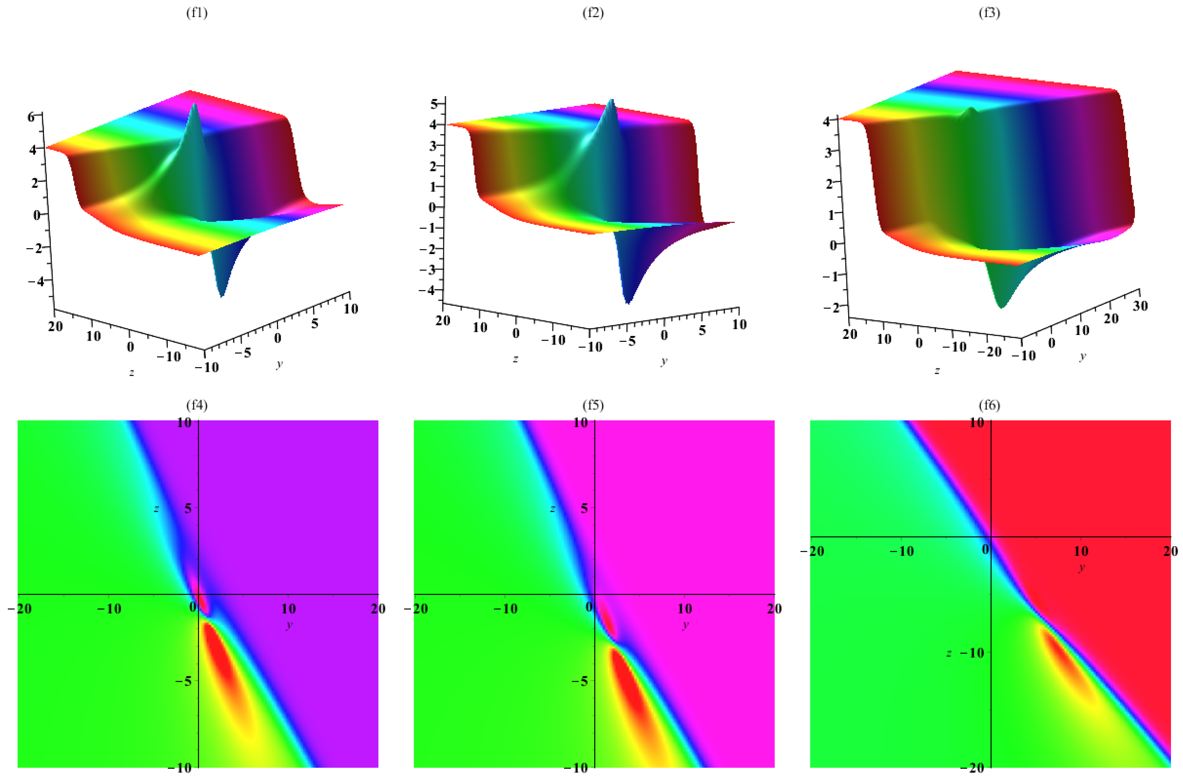
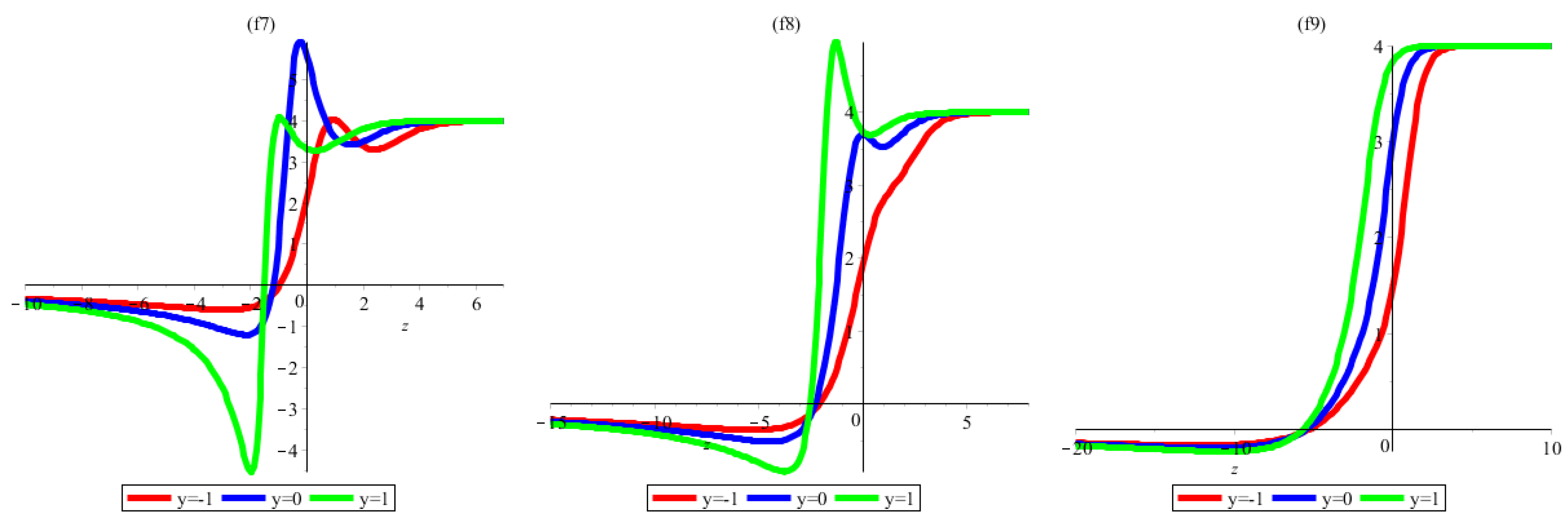
3. Interaction a Lump with One Soliton Solutions

Here, the new exact solutions to the (2+1)-dimensional VC GSWW equation are expressed. Consider the following function for studying the interaction between a lump and one-soliton solutions as

$$h=a_1^2+a_2^2+exp\left(a_3\right)+{\theta }_4\left(t\right),$$

(17)

$$a_k=m_{k}x+n_{k}y+p_{k}z+{\theta }_k\left(t\right),k=1,2,3.$$

Subsequently, the amounts $m_k,n_k,p_k,{\theta }_k\left(t\right)$, (k = 1:4) will be found. By making use of Equation (17) into (16) and taking the coefficients of each power of $exp\left(a_3\right)$ and polynomials to zero, we produced a system of nonlinear equations for $m_k,n_k,p_k,{\theta }_k\left(t\right)$, (k = 1:4). These algebraic equations by using the emblematic computation software, such as Maple software, give the solutions via $\aleph =2{\alpha }_0{(lnh)}_x$ as follows:

$$\aleph =2\frac{{\alpha }_0\left(2\left(m_{1}x+n_{1}y+p_{1}z+{\theta }_1\left(t\right)\right)m_1+2\left(m_{2}x+n_{2}y+p_{2}z+{\theta }_2\left(t\right)\right)m_2+m_3{\mathrm{e}}^{m_{3}x+n_{3}y+p_{3}z+{\theta }_3\left(t\right)}\right)}{{\left(m_{1}x+n_{1}y+p_{1}z+{\theta }_1\left(t\right)\right)}^2+{\left(m_{2}x+n_{2}y+p_{2}z+{\theta }_2\left(t\right)\right)}^2+{\mathrm{e}}^{m_{3}x+n_{3}y+p_{3}z+{\theta }_3\left(t\right)}+{\theta }_4\left(t\right)},$$

$$a_l=m_{l}x+n_{l}y+p_{l}z+{\theta }_l\left(t\right),l=1,2,3.$$

By solving the above received nonlinear system of equations with the aid of Maple, we obtain the following results:

Set I solutions:

$$m_l=0,p_l=\frac{n_l{p}_3}{n_3},{\theta }_l\left(t\right)=C_l,l=1,2,{\theta }_3\left(t\right)=\int -\frac{m_3\left({m_3}^2{n}_3{\alpha }_2\left(t\right)+p_3{\alpha }_4\left(t\right)\right)}{n_3{\alpha }_1\left(t\right)}\mathrm{d}t,{\theta }_4\left(t\right)=C_4,$$

(18)

where $m_3,p_3,n_l,l=1,2,3$ are unknown parameters. According to the logarithm transforation, the rational analytical solution can be introduced as

$${\aleph }_1=\frac{2{\alpha }_0{m}_3{\mathrm{e}}^{m_{3}x+n_{3}y+p_{3}z+\int -\frac{m_3\left({m_3}^2{n}_3{\alpha }_2\left(t\right)+p_3{\alpha }_4\left(t\right)\right)}{n_3{\alpha }_1\left(t\right)}\mathrm{d}t}}{{\left(n_{1}y+\frac{n_1{p}_{3}z}{n_3}+C_1\right)}^2+{\left(n_{2}y+\frac{n_2{p}_{3}z}{n_3}+C_2\right)}^2+{\mathrm{e}}^{m_{3}x+n_{3}y+p_{3}z+\int -\frac{m_3\left({m_3}^2{n}_3{\alpha }_2\left(t\right)+p_3{\alpha }_4\left(t\right)\right)}{n_3{\alpha }_1\left(t\right)}\mathrm{d}t}+C_4}.$$

(19)

Figure 1 shows the analysis of treatment of the interaction between a lump and soliton solution where graphs of ${\mathrm{\Gamma }}_1$ are given with the below selected parameters

$$m_3=1,n_1=n_3=3,n_2=p_3=2,C_1=C_2=C_4=1,{\alpha }_0=2,{\alpha }_1\left(t\right)=t,{\alpha }_2\left(t\right)=t,{\alpha }_4\left(t\right)=-(t^3+2t^2),x=1,$$

(20)

$${\aleph }_1=\frac{4{\mathrm{e}}^{1+3y+2z+2/9t^3+2/3t^2-t}}{{\left(1+3y+2z\right)}^2+{\left(2y+4/3z+1\right)}^2+{\mathrm{e}}^{1+3y+2z+2/9t^3+2/3t^2-t}+1}.$$

From (20), we can see that at any fixed time t, the localized wave and line soliton solution ${\aleph }_1\to 4$ if and only if $a_1^2+a_2^2+exp\left(a_3\right)\to \infty$, namely

$$\underset{y^2+z^2+e^{{\lambda }_{1}y+{\lambda }_{2}z+{\lambda }_3}\to +\infty }{lim}{\aleph }_1=4,{\lambda }_1=3,{\lambda }_2=2,{\lambda }_3=1+2/9t^3+2/3t^2-t,$$

(21)

In order to illustrate the mixed solutions ${\aleph }_2(y,z,t)$ between the localized wave and line soliton solution and one-line soliton solution of VC GSWW Equation, we choose the particular values to the parameters as follows:

$$m_3=1,n_1=n_3=3,n_2=p_3=2,C_1=C_2=C_4=1,{\alpha }_0=2,{\alpha }_1\left(t\right)={\alpha }_4\left(t\right)=exp\left(t\right),{\alpha }_4\left(t\right)=exp\left(2t\right),x=1,$$

(22)

$${\aleph }_1=4\frac{{\mathrm{e}}^{1+3y+2z-{\mathrm{e}}^t-2/3t}}{{\left(1+3y+2z\right)}^2+{\left(2y+4/3z+1\right)}^2+{\mathrm{e}}^{1+3y+2z-{\mathrm{e}}^t-2/3t}+1}.$$

In addition, from (22), we can look that at any fixed time t, the localized wave and line soliton solution ${\aleph }_1\to 1$ if and only if $a_1^2+a_2^2+exp\left(a_3\right)\to \infty$, namely

$$\underset{y^2+z^2+e^{{\lambda }_{1}y+{\lambda }_{2}z+{\lambda }_3}\to +\infty }{lim}{\aleph }_1=1,{\lambda }_1=3,{\lambda }_2=2,{\lambda }_3=1-{\mathrm{e}}^t-2/3t,$$

(23)

in Equation (19). By the above parameters, the structural property interaction between a lump and soliton solution is presented in Figure 1 with density plots with different times. It offers a kind of interaction solutions between polynomial functions and exponential waves. Here, the accomplished lump and soliton solution is presented graphically and contemplated the nature of demonstrated waves for different values of the parameters with the aid of Maple software. We have depicted the physical representations of the derived solutions from the (3+1)-D variable coefficients generalized shallow water wave equation for assorted values of the parameters. The 3D and 2D surface plots of the obtained wave solutions of our discussed equation are addressed here. We have emphasized some values of the constraints of the derived results for which the coefficients of the highest order derivative term and the nonlinear term become reciprocal to each other in the ordinary form of the (3+1)-D variable coefficients generalized shallow water wave equation. From the presented results, we found out that the obtained solutions and effect of the free parameters on the behavior of acquired figure have excellent agreement with the obtained exact solutions in the literature. So, this indicates the efficiency and suitability of the proposed method for solving such models.

Set II solutions:

$$m_1=0,n_3=\frac{n_2{m}_3}{m_2},p_2=\frac{m_2{n_1}^2{p}_3+m_2{n_2}^2{p}_3-n_1{n}_2{p}_1{m}_3}{m_3{n_2}^2},$$

(24)

$${\theta }_1\left(t\right)=\int -\frac{{\alpha }_4\left(t\right)\left(-n_1{p}_3{C}_4{m}_3+m_2{n}_2{p}_1\right)}{{n_2}^2{\alpha }_1\left(t\right)}\mathrm{d}t,{\theta }_2\left(t\right)=\int -\frac{m_3{C}_4{p}_3{\alpha }_4\left(t\right)}{n_2{\alpha }_1\left(t\right)}\mathrm{d}t,$$

$${\alpha }_2\left(t\right)=-\frac{n_1{\alpha }_4\left(t\right)\left(m_2{n}_1{p}_3-n_2{p}_1{m}_3\right)}{3{m_3}^3{n_2}^3},{\theta }_3\left(t\right)=\int \frac{{\alpha }_4\left(t\right)\left(m_2{n_1}^2{p}_3-3m_2{n_2}^2{p}_3-n_1{n}_2{p}_1{m}_3\right)}{3{n_2}^3{\alpha }_1\left(t\right)}\mathrm{d}t,{\theta }_4\left(t\right)=C_4,$$

where $m_2,m_3,p_1,p_3,n_l,$ and $n_2$ are unknown parameters. According to the logarithm transforation, the rational analytical solution can be stated as

$${\aleph }_2=\frac{2{\alpha }_0\left(2Q_2\left(x,y,z,t\right)m_2+m_3{\mathrm{e}}^{Q_3\left(x,y,z,t\right)}\right)}{{\left(n_{1}y+p_{1}z+\int -\frac{{\alpha }_4\left(t\right)\left(-n_1{p}_3{C}_4{m}_3+m_2{n}_2{p}_1\right)}{{n_2}^2{\alpha }_1\left(t\right)}\mathrm{d}t\right)}^2+{\left(Q_2\left(x,y,z,t\right)\right)}^2+{\mathrm{e}}^{Q_3\left(x,y,z,t\right)}+C_4},$$

(25)

along with

$$Q_2\left(x,y,z,t\right)=m_{2}x+n_{2}y+\frac{\left(m_2{n_1}^2{p}_3+m_2{n_2}^2{p}_3-n_1{n}_2{p}_1{m}_3\right)z}{m_3{n_2}^2}+\int -\frac{m_{3}Cj{h}_4{p}_3{\alpha }_4\left(t\right)}{n_2{\alpha }_1\left(t\right)}\mathrm{d}t,$$

$$Q_3\left(x,y,z,t\right)=m_{3}x+\frac{n_2{m}_{3}y}{m_2}+p_{3}z+\int 1/3\frac{{\alpha }_4\left(t\right)\left(m_2{n_1}^2{p}_3-3m_2{n_2}^2{p}_3-n_1{n}_2{p}_1{m}_3\right)}{{n_2}^3{\alpha }_1\left(t\right)}\mathrm{d}t.$$

Figure 1 shows the analysis of treatment of the interaction between a lump and soliton solution where graphs of ${\mathrm{\Gamma }}_1$ are given by using the selected parameters

$$m_2=2,m_3=1,n_1=3,n_2=2,p_1=p_3=2,C_1=C_2=C_4=1,{\alpha }_0=2,{\alpha }_1\left(t\right)=t,{\alpha }_4\left(t\right)=-(t^3+2t^2),x=1,$$

(26)

$${\aleph }_2=4\frac{8+8y+40z+4/3t^3+4t^2+{\mathrm{e}}^{1+y+2z+1/3t^3+t^2}}{{\left(3y+2z+1/6t^3+1/2t^2\right)}^2+{\left(2+2y+10z+1/3t^3+t^2\right)}^2+{\mathrm{e}}^{1+y+2z+1/3t^3+t^2}+1},$$

In order to illustrate the mixed solutions ${\aleph }_2(y,z,t)$ between the localized wave solution and one-line soliton solution of the VC GSWW Equation, we choose the particular values to the parameters as follows:

$$m_2=2,m_3=1,n_1=3,n_2=p_1=p_3=2,C_1=C_2=C_4=1,{\alpha }_0=2,{\alpha }_1\left(t\right)=exp\left(t\right),{\alpha }_4\left(t\right)=exp\left(2t\right),x=1,$$

(27)

$${\aleph }_2=\frac{32+32y+160z-16\frac{{\mathrm{e}}^{2t}}{{\mathrm{e}}^t}+4{\mathrm{e}}^{1+y+2z-\frac{{\mathrm{e}}^{2t}}{{\mathrm{e}}^t}}}{{\left(3y+2z-1/2\frac{{\mathrm{e}}^{2t}}{{\mathrm{e}}^t}\right)}^2+{\left(2+2y+10z-\frac{{\mathrm{e}}^{2t}}{{\mathrm{e}}^t}\right)}^2+{\mathrm{e}}^{1+y+2z-\frac{{\mathrm{e}}^{2t}}{{\mathrm{e}}^t}}+1},$$

in Equation (25). By the above parameters, the structural property interaction between a lump and soliton solution is presented in Figure 2 with density plots with different times. It shows a kind of interaction solutions between polynomial functions and exponential waves. From (27), we can look that at any fixed time t, the localized wave and line soliton solution ${\aleph }_1\to 1$ if and only if $a_1^2+a_2^2+exp\left(a_3\right)\to \infty$, namely

$$\underset{y^2+z^2+e^{{\lambda }_{1}y+{\lambda }_{2}z+{\lambda }_3}\to +\infty }{lim}{\aleph }_2=1,{\lambda }_1=1,{\lambda }_2=2,{\lambda }_3=1-{\mathrm{e}}^t.$$

(28)

Set III solutions:

$$m_1=0,n_2=-1/4\frac{{m_3}^3{n_1}^2{C}_4\left({m_3}^2{C}_4-2{m_2}^2\right)}{\left(-{m_3}^2{s}_4+{m_2}^2\right){m_2}^3{n}_3},$$

(29)

$$p_2=\frac{m_2\left({m_3}^2{p}_3{C}_4{n}_1-2n_3{m_3}^2{p}_1{C}_4-2{m_2}^2{p}_3{n}_1+2{m_2}^2{n}_3{p}_1\right)}{\left({m_3}^2{C}_4-2{m_2}^2\right)n_1{m}_3},$$

$${\alpha }_2\left(t\right)=-4/3\frac{{\alpha }_4\left(t\right)\left({m_3}^2{p}_3{C}_4{n}_1-n_3{m_3}^2{p}_1{C}_4-{m_2}^2{p}_3{n}_1+{m_2}^2{n}_3{p}_1\right)}{n_1{m_3}^2\left({m_3}^2{C}_4-2{m_2}^2\right)n_3},$$

$${\theta }_1\left(t\right)=\int -4\frac{{\alpha }_4\left(t\right)\left(n_1{p}_3-n_3{p}_1\right){m_2}^4\left(C_4{m_3}^2-{m_2}^2\right)}{{n_1}^2{m}_3\left({C_4}^2{m_3}^4-4C_4{m_2}^2{m_3}^2+4{m_2}^4\right){\alpha }_1\left(t\right)}\mathrm{d}t,$$

$${\alpha }_2\left(t\right)=\int \frac{{\alpha }_4\left(t\right)\left(C_4{m_3}^2{n}_1{p}_3-2C_4{m_3}^2{n}_3{p}_1+2{m_2}^2{n}_3{p}_1\right)m_2}{n_1\left(C_4{m_3}^2-2{m_2}^2\right)n_3{\alpha }_1\left(t\right)}\mathrm{d}t,$$

and

$${\theta }_3\left(t\right)=\int \frac{{\alpha }_4\left(t\right)\left(C_4{m_3}^2{n}_1{p}_3-4C_4{m_3}^2{n}_3{p}_1+2{m_2}^2{n}_1{p}_3+4{m_2}^2{n}_3{p}_1\right)m_3}{3n_1\left(C_4{m_3}^2-2{m_2}^2\right)n_3{\alpha }_1\left(t\right)}\mathrm{d}t,{\theta }_4\left(t\right)=C_4,$$

where $m_2,m_3,p_1,p_3,n_l,$ and $n_3$ are free values. According to the logarithm transforation, the rational analytical solution can be shown as

$${\aleph }_3=\frac{2{\alpha }_0\left(2Q_2\left(x,y,z,t\right)m_2+m_3{\mathrm{e}}^{Q_3\left(x,y,z,t\right)}\right)}{{\left(n_{1}y+p_{1}z+\int -4\frac{{\alpha }_4\left(t\right)\left(n_1{p}_3-n_3{p}_1\right){m_2}^4\left(C_4{m_3}^2-{m_2}^2\right)}{{n_1}^2{m}_3\left({C_4}^2{m_3}^4-4C_4{m_2}^2{m_3}^2+4{m_2}^4\right){\alpha }_1\left(t\right)}\mathrm{d}t\right)}^2+{\left(Q_2\left(x,y,z,t\right)\right)}^2+{\mathrm{e}}^{Q_3\left(x,y,z,t\right)}+C_4},$$

(30)

along with

$$Q_2\left(x,y,z,t\right)=m_{2}x-\frac{{m_3}^3{n_1}^2{C}_4\left(C_4{m_3}^2-2{m_2}^2\right)y}{4\left(-{m_3}^2{C}_4+{m_2}^2\right){m_2}^3{n}_3}+\frac{m_2\left(C_4{m_3}^2{n}_1{p}_3-2C_4{m_3}^2{n}_3{p}_1-2{m_2}^2{n}_1{p}_3+2{m_2}^2{n}_3{p}_1\right)z}{n_1\left(C_4{m_3}^2-2{m_2}^2\right)m_3}$$

$$+\int \frac{{\alpha }_4\left(t\right)\left(C_4{m_3}^2{n}_1{p}_3-2C_4{m_3}^2{n}_3{p}_1+2{m_2}^2{n}_3{p}_1\right)m_2}{n_1\left(C_4{m_3}^2-2{m_2}^2\right)n_3{\alpha }_1\left(t\right)}\mathrm{d}t,$$

$$Q_3\left(x,y,z,t\right)=m_{3}x+n_{3}y+p_{3}z+\int 1/3\frac{{\alpha }_4\left(t\right)\left(C_4{m_3}^2{n}_1{p}_3-4C_4{m_3}^2{n}_3{p}_1+2{m_2}^2{n}_1{p}_3+4{m_2}^2{n}_3{p}_1\right)m_3}{n_1\left(C_4{m_3}^2-2{m_2}^2\right)n_3{\alpha }_1\left(t\right)}\mathrm{d}t.$$

Figure 3 shows the analysis of treatment of interaction between a lump and soliton solution where graphs of ${\mathrm{\Gamma }}_1$ are given with the below selected parameters

$$m_2=2,m_3=1,n_1=3,n_3=p_1=p_3=2,C_1=C_2=C_4=1,{\alpha }_0=2,{\alpha }_1\left(t\right)=t,{\alpha }_4\left(t\right)=-(t^3+2t^2),x=1,$$

(31)

$${\aleph }_3=\frac{32+\frac{21y}{4}+\frac{192z}{7}+\frac{160t^3}{21}+\frac{160t^2}{7}+4{\mathrm{e}}^{1+2y+2z+\frac{17t^3}{63}+\frac{17t^2}{21}}}{{\left(3y+2z-\frac{128t^3}{441}-\frac{128t^2}{147}\right)}^2+{\left(2+\frac{21y}{64}+\frac{12z}{7}+\frac{10t^3}{21}+\frac{10t^2}{7}\right)}^2+{\mathrm{e}}^{1+2y+2z+\frac{17t^3}{63}+\frac{17t^2}{21}}+1},$$

and

$$m_2=2,m_3=1,n_1=3,n_3=p_1=p_3=2,C_1=C_2=C_4=1,{\alpha }_0=2,{\alpha }_1\left(t\right)=exp\left(t\right),{\alpha }_4\left(t\right)=exp\left(2t\right),x=1,$$

(32)

$${\aleph }_3=\frac{32+\frac{21y}{4}+\frac{192z}{7}-\frac{160{\mathrm{e}}^{2t}}{7{\mathrm{e}}^t}+4{\mathrm{e}}^{1+2y+2z-\frac{17{\mathrm{e}}^{2t}}{21{\mathrm{e}}^t}}}{{\left(3y+2z+\frac{128{\mathrm{e}}^{2t}}{147{\mathrm{e}}^t}\right)}^2+{\left(2+\frac{21y}{64}+\frac{12z}{7}-\frac{10{\mathrm{e}}^{2t}}{7{\mathrm{e}}^t}\right)}^2+{\mathrm{e}}^{1+2y+2z-\frac{17{\mathrm{e}}^{2t}}{21{\mathrm{e}}^t}}+1},$$

(33)

in Equation (30). By the above parameters, the structural property interaction between a lump and soliton solution is presented in Figure 3 with density plots with different times. It shows a kind of interaction solution between two positive quadratic functions and hyperbolic waves. Figure 3 shows the dynamic processes of the mixed solution corresponding to (33). It shows the 3D graph and 2D plot in the $(y;z)$ plane when $x=1$, respectively. The 3D graphs and the 2D plots showed the localized structures and the energy distribution of the mixed solution, respectively. We can see that the localized wave and line soliton solution interact with each other and move forward in the y direction.

Set IV solutions:

$${\aleph }_4=\frac{4{\alpha }_0\left(m_{2}x-\int \frac{m_2{\alpha }_4\left(t\right)p_3}{n_3{\alpha }_1\left(t\right)}\mathrm{d}t\right)m_2}{{\left(n_{1}y+\frac{n_1{p}_{3}z}{n_3}+C_1\right)}^2+{\left(m_{2}x-\int \frac{m_2{\alpha }_4\left(t\right)p_3}{n_3{\alpha }_1\left(t\right)}\mathrm{d}t\right)}^2+{\mathrm{e}}^{n_{3}y+p_{3}z+C_3}+C_4},$$

(34)

and

$${\aleph }_5=\frac{2{\alpha }_0{m}_3{\mathrm{e}}^{m_{3}x+n_{3}y+p_{3}z+\int -\frac{{m_3}^3{\alpha }_2\left(t\right)}{{\alpha }_1\left(t\right)}\mathrm{d}t}}{{\left(n_{1}y+p_{1}z+C_1\right)}^2+{\left(y{n}_2+z{p}_2+C_2\right)}^2+{\mathrm{e}}^{m_{3}x+n_{3}y+p_{3}z+\int -\frac{{m_3}^3{\alpha }_2\left(t\right)}{{\alpha }_1\left(t\right)}\mathrm{d}t}+C_4}.$$

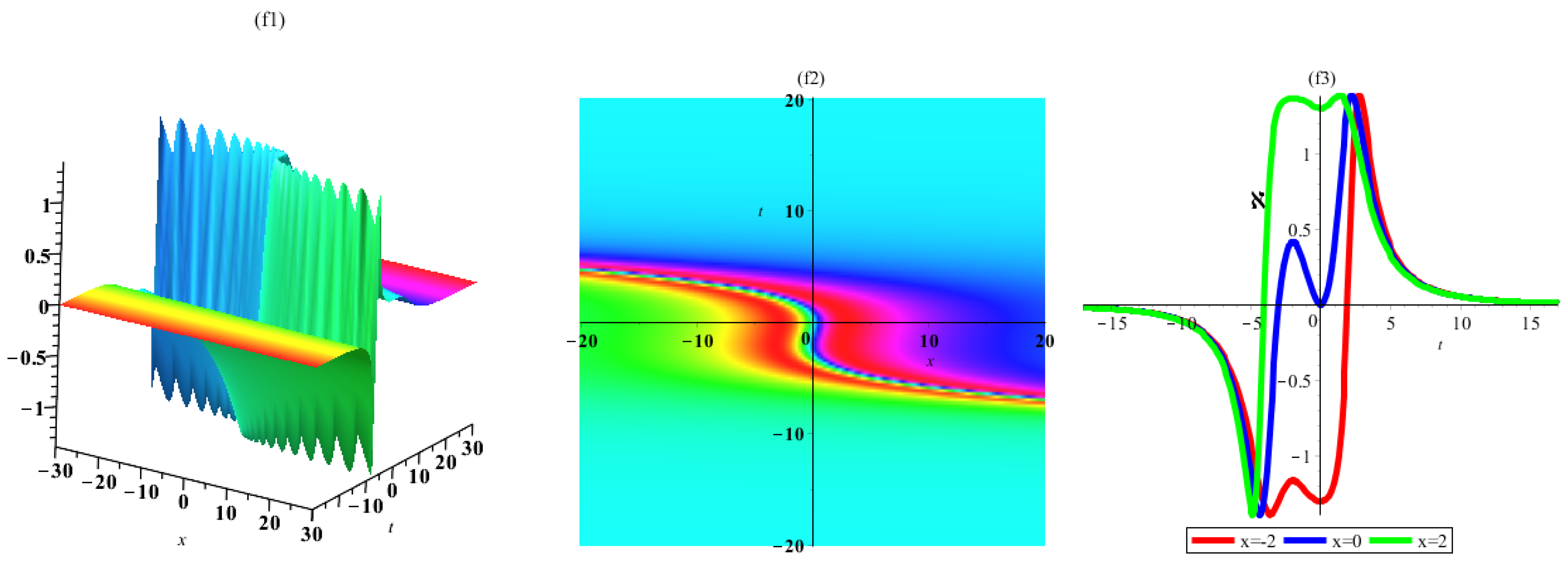
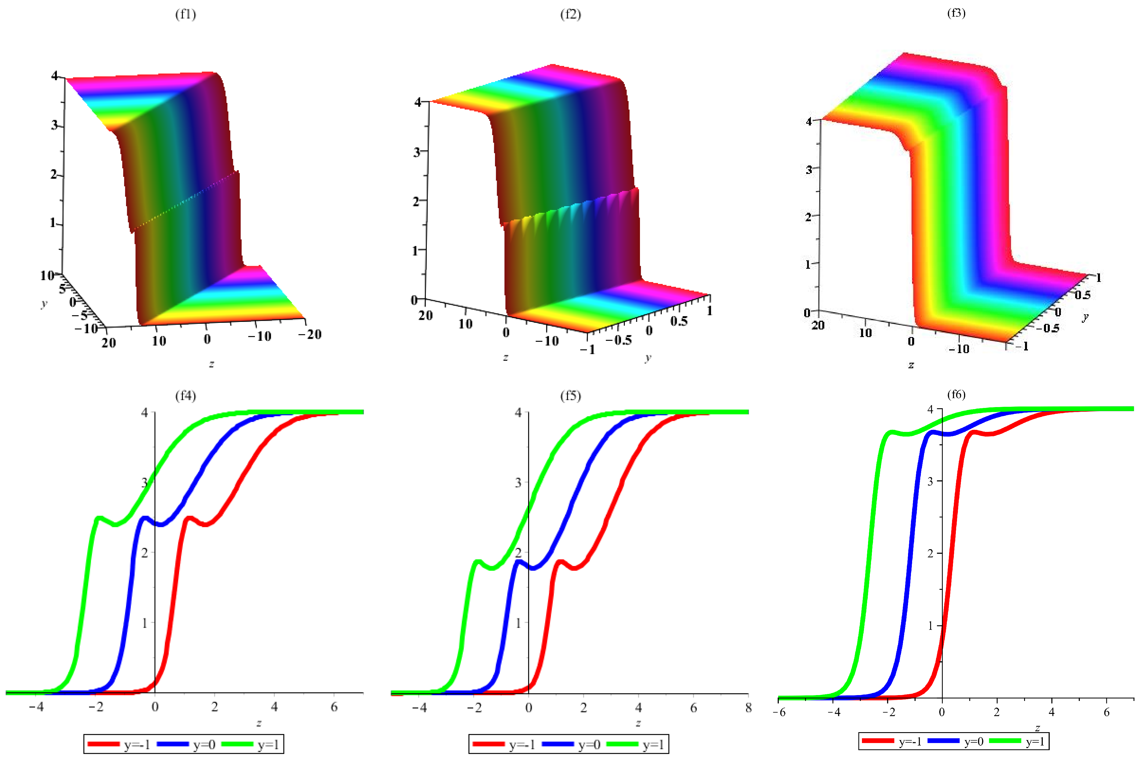
4. Interaction a Lump with Two Soliton Solutions

This section describes finding the new exact solutions to the (2+1)-dimensional VC GSWW equation. Consider the following function for studying the interaction of a lump with two-soliton solutions as

$$h=a_1^2+a_2^2+cosh\left(a_3\right)+sinh\left(a_4\right)+{\theta }_5\left(t\right),$$

(35)

$$a_k=m_{k}x+n_{k}y+p_{k}z+{\theta }_k\left(t\right),k=1,2,3,4.$$

Then, the values $m_k,n_k,p_k,{\theta }_k\left(t\right)$, and ($l=k$:4) will be found. By making use of Equation (35) into (16) and taking the coefficients the each powers of $cosh\left(a_3\right),cosh\left(a_4\right),sinh\left(a_3\right),sinh\left(a_4\right)$ and polynomials to zero, we produced a system of nonlinear equations for $m_k,n_k,p_k,{\theta }_k\left(t\right)$, (k = 1:4). Based on the $\mathrm{\Sigma }=2{\alpha }_0{(lnh)}_x$, we obtain:

$$\aleph =2\frac{{\alpha }_0\left(2a_1{m}_1+2a_2{m}_2+sinh\left(a_3\right)m_3+cosh\left(a_4\right)m_4\right)}{{a_1}^2+{a_2}^2+cosh\left(a_3\right)+sinh\left(a_4\right)+{\theta }_5\left(t\right)},$$

$$a_l=m_{l}x+n_{l}y+p_{l}z+{\theta }_l\left(t\right),l=1,2,3,4.$$

Set I solutions:

$$m_l=0,l=1,3,4,n_l=0,l=2,3,p_l=0,l=2,3,p_1=\frac{p_4{n}_1}{n_4},{\theta }_1\left(t\right)=C_1,$$

(36)

$${\theta }_2\left(t\right)=\int -\frac{{\alpha }_4\left(t\right)m_2{p}_4}{{\alpha }_1\left(t\right)n_4}\mathrm{d}t,{\theta }_3\left(t\right)=C_3,{\theta }_4\left(t\right)=C_4,{\theta }_5\left(t\right)=C_5,$$

where $m_2,p_4,n_l,$ and $l=1,4$ are free amounts. According to the logarithm transforation, the rational analytical solution can be expressed as

$${\aleph }_1=\frac{4{\alpha }_0\left(m_{2}x+\int -\frac{{\alpha }_4\left(t\right)m_2{p}_4}{{\alpha }_1\left(t\right)n_4}\mathrm{d}t\right)m_2}{{\left(n_{1}y+\frac{n_1{p}_{4}z}{n_4}+C_1\right)}^2+{\left(m_{2}x+\int -\frac{{\alpha }_4\left(t\right)m_2{p}_4}{{\alpha }_1\left(t\right)n_4}\mathrm{d}t\right)}^2+cosh\left(C_3\right)+sinh\left(n_{4}y+p_{4}z+C_4\right)+C_5}.$$

(37)

Set II solutions:

$$m_l=0,l=3,4,n_l=0,l=1,2,3,p_l=0,l=1,2,3,$$

(38)

$${\theta }_1\left(t\right)=-\frac{{\theta }_2\left(t\right)m_2}{m_1}-\frac{m_2}{m_1}\int \frac{{\alpha }_4\left(t\right){m_1}^2{p}_4}{{\alpha }_1\left(t\right)n_4{m}_2}+\frac{{\alpha }_4\left(t\right)m_2{p}_4}{{\alpha }_1\left(t\right)n_4}\mathrm{d}t,{\theta }_2\left(t\right)={\theta }_2\left(t\right),{\theta }_3\left(t\right)=C_3,{\theta }_4\left(t\right)=C_4,$$

$${\theta }_5\left(t\right)=-{\left({\theta }_2\left(t\right)\right)}^2+\int 2\frac{\left(\frac{\mathrm{d}}{\mathrm{d}t}{\theta }_2\left(t\right)\right)m_2{\theta }_1\left(t\right)}{m_1}\mathrm{d}t+\int -2\frac{{\alpha }_4\left(t\right)m_2{p}_4{\theta }_2\left(t\right)m_1-{\alpha }_4\left(t\right){m_2}^2{p}_4{\theta }_1\left(t\right)}{{\alpha }_1\left(t\right)m_1{n}_4}\mathrm{d}t,$$

where $m_1,m_2,p_4,$ and $n_4,$ are free amounts. According to the logarithm transforation, the rational exact solution can be introduced as

$${\aleph }_2=2\frac{{\alpha }_0\left(2Q_1\left(x,t\right)m_1+2\left(m_{2}x+{\theta }_2\left(t\right)\right)m_2\right)}{{\left(Q_1\left(x,t\right)\right)}^2+{\left(m_{2}x+{\theta }_2\left(t\right)\right)}^2+cosh\left(C_3\right)+sinh\left(n_{4}y+p_{4}z+C_4\right)+Q_5\left(t\right)},$$

(39)

along with

$$Q_1\left(x,t\right)=m_{1}x-\frac{{\theta }_2\left(t\right)m_2}{m_1}-\frac{m_2}{m_1}\int \frac{{\alpha }_4\left(t\right){m_1}^2{p}_4}{{\alpha }_1\left(t\right)n_4{m}_2}+\frac{{\alpha }_4\left(t\right)m_2{p}_4}{{\alpha }_1\left(t\right)n_4}\mathrm{d}t,$$

$$Q_5\left(t\right)=-{\left({\theta }_2\left(t\right)\right)}^2+\int 2\frac{\left(\frac{\mathrm{d}}{\mathrm{d}t}{\theta }_2\left(t\right)\right)m_2{\theta }_1\left(t\right)}{m_1}\mathrm{d}t+\int -2\frac{{\alpha }_4\left(t\right)m_2{p}_4{\theta }_2\left(t\right)m_1-{\alpha }_4\left(t\right){m_2}^2{p}_4{\theta }_1\left(t\right)}{{\alpha }_1\left(t\right)m_1{n}_4}\mathrm{d}t.$$

Set III solutions:

$$m_l=0,l=3,4,n_1=-\frac{m_2{n}_4{p}_2}{p_4{m}_1},n_2=\frac{n_4{p}_2}{p_4},n_3=0,p_1=-\frac{m_2{p}_2}{m_1},p_3=0,$$

(40)

$${\theta }_1\left(t\right)=\int -\frac{{\alpha }_4\left(t\right)m_1{p}_4}{{\alpha }_1\left(t\right)n_4}\mathrm{d}t,{\theta }_2\left(t\right)=\int -\frac{{\alpha }_4\left(t\right)m_2{p}_4}{{\alpha }_1\left(t\right)n_4}\mathrm{d}t,{\theta }_3\left(t\right)=C_3,{\theta }_4\left(t\right)=C_4,{\theta }_5\left(t\right)=C_5,$$

where $m_1,m_2,p_2,$ and $n_4,$ are free amounts. According to the logarithm transforation, the exact solution can be written as

$${\aleph }_3=2\frac{{\alpha }_0\left(2Q_1\left(x,y,z,t\right)m_1+2Q_2\left(x,y,z,t\right)m_2\right)}{{\left(Q_1\left(x,y,z,t\right)\right)}^2+{\left(Q_2\left(x,y,z,t\right)\right)}^2+cosh\left(C_3\right)+sinh\left(n_{4}y+p_{4}z+C_4\right)+C_5},$$

(41)

along with

$$Q_1\left(x,y,z,t\right)=m_{1}x-\frac{m_2{n}_4{p}_{2}y}{p_4{m}_1}-\frac{m_2{p}_{2}z}{m_1}+\int -\frac{{\alpha }_4\left(t\right)m_1{p}_4}{{\alpha }_1\left(t\right)n_4}\mathrm{d}t,$$

$$Q_2\left(x,y,z,t\right)=m_{2}x+\frac{n_4{p}_{2}y}{p_4}+p_{2}z+\int -\frac{{\alpha }_4\left(t\right)m_2{p}_4}{{\alpha }_1\left(t\right)n_4}\mathrm{d}t.$$

From (41), we can look that at any fixed time t and space x, the localized wave and solitary wave solutions ${\aleph }_3\to 0$ if and only if $a_1^2+a_2^2+cosh\left(a_3\right)+sinh\left(a_4\right)\to \infty$, namely

$$\underset{y^2+z^2+cosh(y,z)+sinh(y,z)\to +\infty }{lim}=0,$$

(42)

Figure 4 shows the analysis of treatment of interaction between a lump and two-soliton solution where graphs of ${\mathrm{\Gamma }}_3$ are given with the below selected parameters

$$m_1=1,m_2=2,n_4=3,p_2=2,p_4=C_3=C_4=C_5=1,{\alpha }_0=2,{\alpha }_1\left(t\right)=-t,{\alpha }_4\left(t\right)=(t^3+2t^2),y=0.2,z=-2,$$

(43)

$${\aleph }_3=4\frac{\left(10x+\frac{10t^3}{9}+10/3t^2\right)}{{\left(x+5.6+1/9t^3+1/3t^2\right)}^2+{\left(2x-2.8+2/9t^3+2/3t^2\right)}^2+cosh\left(1\right)+0.5892476742},$$

(44)

in Equation (41). By the above parameters, the structural property interaction between a lump and two-soliton solution is presented in Figure 4 with density plots with different spaces. It shows a kind of interaction solutions between two positive quadratic functions and two hyperbolic waves. The dynamic analysis and properties for the mixed solution corresponding to (44) are shown in Figure 4. It shows the Figure 4 3D plots and 2D plots at times $y=0.2,z=-2$. The 3D dynamic graph, density and 2D plot are in the $(x;t)$-plane when $y=0.2,z=-2$, respectively. The 3D graphs and the density plots showed the localized structures and the energy distribution of the mixed solution, respectively. We can see that the localized wave and other wave interact with each other and keep moving forward.

Set IV solutions:

$$m_l=0,l=1,3,n_1=n_1,p_l=0,l=2,3,4,{\theta }_1\left(t\right)=C_1,$$

(45)

$${\theta }_2\left(t\right)=\int -\frac{m_2{\alpha }_4\left(t\right)p_1}{n_1{\alpha }_1\left(t\right)}\mathrm{d}t,{\theta }_3\left(t\right)=C_3,{\theta }_4\left(t\right)=\int -\frac{m_4\left({\alpha }_2\left(t\right){m_4}^2{n}_1+{\alpha }_4\left(t\right)p_1\right)}{n_1{\alpha }_1\left(t\right)}\mathrm{d}t,{\theta }_5\left(t\right)=C_5,$$

where $m_2,m_4,p_1,$ and $n_1,$ are unknown parameters. According to the logarithm transforation, the rational analytical solution can be found as

$${\aleph }_4=\frac{2{\alpha }_0\left(2\left(m_{2}x+\int -\frac{{\alpha }_4\left(t\right)m_2{p}_1}{n_1{\alpha }_1\left(t\right)}\mathrm{d}t\right)m_2+cosh\left(m_{4}x+\int -\frac{m_4\left({\alpha }_2\left(t\right){m_4}^2{n}_1+{\alpha }_4\left(t\right)p_1\right)}{n_1{\alpha }_1\left(t\right)}\mathrm{d}t\right)m_4\right)}{{\left(n_{1}y+p_{1}z+C_1\right)}^2+{\left(m_{2}x+\int -\frac{{\alpha }_4\left(t\right)m_2{p}_1}{n_1{\alpha }_1\left(t\right)}\mathrm{d}t\right)}^2+cosh\left(C_3\right)+sinh\left(m_{4}x+\int -\frac{m_4\left({\alpha }_2\left(t\right){m_4}^2{n}_1+{\alpha }_4\left(t\right)p_1\right)}{n_1{\alpha }_1\left(t\right)}\mathrm{d}t\right)+C_5}.$$

(46)

Set V solutions:

$$m_l=0,l=1,2,4,n_1=-n_2,p_1=-p_2,p_l=0,l=3,4,$$

(47)

$${\theta }_2\left(t\right)=-{\theta }_1\left(t\right),{\theta }_3\left(t\right)=C_3,{\theta }_4\left(t\right)=\int -\frac{m_4\left({\alpha }_2\left(t\right){m_4}^2{n}_2+p_2{\alpha }_4\left(t\right)\right)}{n_2{\alpha }_1\left(t\right)}\mathrm{d}t,{\theta }_5\left(t\right)=C_5,$$

where $m_2,m_4,p_1,$ and $n_1,$ are free values. According to the logarithm transforation, the rational analytical solution can be shown as

$${\aleph }_5=2\frac{{\alpha }_0\left(2Q_2\left(x,t\right)m_2+cosh\left(Q_4\left(x,t\right)\right)m_4\right)}{{\left(n_{1}y+p_{1}z+C_1\right)}^2+{\left(Q_2\left(x,t\right)\right)}^2+cosh\left(C_3\right)+\left(sinh\right)Q_4\left(x,t\right)+C_5},$$

(48)

along with

$$Q_2\left(x,t\right)=m_{2}x+\int -\frac{{\alpha }_4\left(t\right)m_2{p}_1}{n_1{\alpha }_1\left(t\right)}\mathrm{d}t,$$

$$Q_4\left(x,t\right)=m_{4}x+\int -\frac{m_4\left({\alpha }_2\left(t\right){m_4}^2{n}_1+{\alpha }_4\left(t\right)p_1\right)}{n_1{\alpha }_1\left(t\right)}\mathrm{d}t.$$

Set VI solutions:

$$m_l=0,l=1,2,3,n_l=0,p_1=\frac{n_1{p}_2}{n_2},p_l=0,l=3,4,{\theta }_2\left(t\right)=-\frac{{\theta }_1\left(t\right)n_1}{n_2},{\theta }_3\left(t\right)=C_3,$$

(49)

$${\theta }_4\left(t\right)=\int -\frac{m_4\left({\alpha }_2\left(t\right){m_4}^2{n}_2+p_2{\alpha }_4\left(t\right)\right)}{{\alpha }_1\left(t\right)n_2}\mathrm{d}t,{\theta }_5\left(t\right)=\int 2\frac{\left(n_1{\theta }_2\left(t\right)-n_2{\theta }_1\left(t\right)\right)\frac{\mathrm{d}}{\mathrm{d}t}{\theta }_1\left(t\right)}{n_2}\mathrm{d}t,$$

where $m_4,p_2,n_1,$ and $n_2,$ are unknown parameters. According to the logarithm transforation, the rational analytical solution can be expressed as

$${\aleph }_6=\frac{2{\alpha }_{0}cosh\left(Q_4\left(x,t\right)\right)m_4}{{\left(n_{1}y+\frac{n_1{p}_{2}z}{n_2}+{\theta }_1\left(t\right)\right)}^2+{\left(n_{2}y+p_{2}z-\frac{{\theta }_1\left(t\right)n_1}{n_2}\right)}^2+cosh\left(C_3\right)+sinh\left(Q_4\left(x,t\right)\right)+Q_5\left(t\right)},$$

(50)

along with

$$Q_4\left(x,t\right)=m_{4}x+\int -\frac{m_4\left({\alpha }_2\left(t\right){m_4}^2{n}_2+p_2{\alpha }_4\left(t\right)\right)}{{\alpha }_1\left(t\right)n_2}\mathrm{d}t,$$

$$Q_5\left(t\right)=\int 2\frac{\left(n_1{\theta }_2\left(t\right)-n_2{\theta }_1\left(t\right)\right)\frac{\mathrm{d}}{\mathrm{d}t}{\theta }_1\left(t\right)}{n_2}\mathrm{d}t.$$

Set VII solutions:

$$m_2=-\frac{m_1{n}_1}{n_2},m_3=0,n_l=0,p_1=\frac{n_1{p}_2}{n_2},p_l=0,l=3,4,{\theta }_1\left(t\right)=\int -\frac{{\alpha }_4\left(t\right)m_1{p}_2}{{\alpha }_1\left(t\right)n_2}\mathrm{d}t,$$

(51)

$${\theta }_2\left(t\right)=\int \frac{{\alpha }_4\left(t\right)m_1{n}_1{p}_2}{{\alpha }_1\left(t\right){n_2}^2}\mathrm{d},{\theta }_3\left(t\right)=C_3,{\theta }_4\left(t\right)=\int -\frac{m_4\left({\alpha }_2\left(t\right){m_4}^2{n}_2+p_2{\alpha }_4\left(t\right)\right)}{{\alpha }_1\left(t\right)n_2}\mathrm{d}t,{\theta }_5\left(t\right)=C_5,$$

where $m_1,m_4,p_2,n_1,$ and $n_2,$ are free parameters. According to the logarithm transforation, the rational analytical solution can be specified as

$${\aleph }_7=2\frac{{\alpha }_0\left(2Q_1\left(x,y,z,t\right)m_1-2\frac{Q_2\left(x,y,z,t\right)m_1{n}_1}{n_2}+cosh\left(Q_4\left(x,y,z,t\right)\right)m_4\right)}{{\left(Q_1\left(x,y,z,t\right)\right)}^2+{\left(Q_2\left(x,y,z,t\right)\right)}^2+cosh\left(C_3\right)+sinh\left(Q_4\left(x,y,z,t\right)\right)+C_5},$$

(52)

along with

$$Q_1\left(x,y,z,t\right)=m_{1}x+n_{1}y+\frac{n_1{p}_{2}z}{n_2}+\int -\frac{{\alpha }_4\left(t\right)m_1{p}_2}{{\alpha }_1\left(t\right)n_2}\mathrm{d}t,$$

$$Q_2\left(x,y,z,t\right)=-\frac{m_1{n}_{1}x}{n_2}+n_{2}y+p_{2}z+\int \frac{{\alpha }_4\left(t\right)m_1{n}_1{p}_2}{{\alpha }_1\left(t\right){n_2}^2}\mathrm{d}t,$$

$$Q_4\left(x,y,z,t\right)=m_{4}x+\int -\frac{m_4\left({\alpha }_2\left(t\right){m_4}^2{n}_2+p_2{\alpha }_4\left(t\right)\right)}{{\alpha }_1\left(t\right)n_2}\mathrm{d}t.$$

For evading repetitions, we have appended a similar type of figure once obtained from different wave solutions in our study.

5. Conclusions

This article investigated the interaction between a lump and one- or two-soliton solutions to the (3+1)-D VC generalized shallow water wave equation. The bilinear form of the equation has been described by means of algorithm transformation. The interactions between a lump and one- or two-soliton solutions containing more cases of solutions were obtained. We found a combination of two-kinks rational solutions for interaction between a lump and one- or two-soliton solutions of the governing equation. It shows a kind of interaction of solutions between positive quadratic functions and hyperbolic waves for the obtained solutions. The dynamic features of distinctive kinds of traveling waves are analyzed in detail by a numerical simulation. At the same time, the profiles of the surface for the deduced solutions have been designed in 3D, 2D, and density plots for free amounts. The implemented method can also be applied to analyze numerous nonlinear evolution equations in applied mathematics and mathematical physics, which will be explored in future work. Furthermore, the acquired solutions reveal that the method we have deliberated here is a competent mathematical tool for furnishing a variety of new exact traveling wave solutions with the free parameter of different physical structures.

References

1. Randall, D.A. The Shallow Water Equations; Technical Report; Atmospheric Science, Colorado State University: Fort Collins, CO, USA, 2006. [Google Scholar]
2. Shinbrot, M. The shallow water equations. J. Eng. Math. 1970, 4, 293–304. [Google Scholar] [CrossRef]
3. Klimachkov, D.A.; Petrosyan, A.S. Rossby waves in the magnetic fluid dynamics of a rotating plasma in the shallow-water approximation. J. Exp. Theor. Phys. 2017, 125, 597–612. [Google Scholar] [CrossRef]
4. Zayed, E.M.E. Traveling wave solutions for higher dimensional nonlinear evolution equations using the (G’/G) expansion method. J. Appl. Math. Inf. 2010, 28, 383–395. [Google Scholar]
5. Tang, Y.N.; Ma, W.X.; Xu, W. Grammian and Pfaffian solutions as well as pfaffianization for a (3+1)-dimensional generalized shallow water equation. Chin. Phys. B 2012, 21, 070212. [Google Scholar] [CrossRef]
6. Liu, J.G.; Zhou, L.; He, Y. Multiple soliton solutions for the new (2+1)-dimensional Korteweg-de Vries equation by multiple exp-function method. Appl. Math. Lett. 2018, 80, 71–78. [Google Scholar] [CrossRef]
7. Noori, A.W.; Royen, M.J.; Haydary, J. Thin-layer mathematical modeling of apple slices drying, using open sun and cabinet solar drying methods. Int. J. Innov. Sci. Stud. 2021, 4, 43–52. [Google Scholar] [CrossRef]
8. Chen, S.; Zhang, J.; Meng, F.; Wang, D.; Wei, Z.; Zhang, W. A Markov Chain Position Prediction Model Based on Multidimensional Correction. Complexity 2021, 2021, 6677132. [Google Scholar] [CrossRef]
9. Zhou, Y.; Wang, C.; Zhang, X. Rational Localized Waves and Their Absorb-Emit Interactions in the (2+1)-Dimensional Hirota–Satsuma–Ito Equation. Mathematics 2020, 8, 1807. [Google Scholar] [CrossRef]
10. Srinivasareddy, S.; Narayana, Y.V.; Krishna, D. Sector Beam Synthesis in Linear Antenna Arrays using Social Group Optimization Algorithm. Natl. J. Antennas Propag. 2021, 3, 6–9. [Google Scholar]
11. Wickramasinghe, K. The Use of Deep Data Locality towards a Hadoop Performance Analysis Framework. Int. J. Commun. Comput. Technol. 2020, 8, 5–8. [Google Scholar]
12. Xiao, Y.; Fan, E.; Liu, P. Inverse scattering transform for the coupled modified Korteweg–de Vries equation with nonzero boundary conditions. J. Math. Anal. Appl. 2021, 504, 125567. [Google Scholar] [CrossRef]
13. Zhou, G.; Zhang, R.; Huang, S. Generalized Buffering Algorithm. IEEE Access 2021, 9, 27140–27157. [Google Scholar] [CrossRef]
14. Wen, X.Y.; Xu, X.G. Multiple soliton solutions and fusion interaction phenomena for the (2+1)-dimensional modified dispersive water-wave system. Appl. Math. Comput. 2013, 219, 7730–7740. [Google Scholar] [CrossRef]
15. Svilović, S.; Zelić, J. Comparison of Non-Linear and Linear Ho Models Applied for Copper Ions Sorption on Geopolymer. Teh. Glas. 2021, 15, 305–309. [Google Scholar]
16. Liu, X.; Zhang, G.; Li, J.; Shi, G.; Zhou, M.; Huang, B.; Yang, W. Deep Learning for Feynman’s Path Integral in Strong-Field Time-Dependent Dynamics. Phys. Rev. Lett. 2020, 124, 113202. [Google Scholar] [CrossRef] [PubMed]
17. Cai, L.; Xiong, L.; Cao, J.; Zhang, H.; Alsaadi, F.E. State quantized sampled-data control design for complex-valued memristive neural networks. J. Frankl. Inst. 2020. [Google Scholar] [CrossRef]
18. Liu, S.; He, X.; Chan, F.T.S.; Wang, Z. An Extended Multi-Criteria Group Decision-Making Method with Psychological Factors and Bidirectional Influence Relation for Emergency Medical Supplier Selection. Expert Syst. Appl. 2022, 202, 117414. [Google Scholar] [CrossRef]
19. Meng, F.; Pang, A.; Dong, X.; Han, C.; Sha, X.; Jing, N.; Na, J. H Optimal Performance Design of an Unstable Plant under Bode Integral Constraint. Complexity 2018, 2018, 4942906. [Google Scholar] [CrossRef]
20. Meng, F.; Wang, D.; Yang, P.; Xie, G.; Cutberto, R.; Romero-Melendez, C. Application of Sum of Squares Method in Nonlinear H Control for Satellite Attitude Maneuvers. Complexity 2019, 2019, 5124108. [Google Scholar] [CrossRef]
21. Tian, H.; Huang, N.; Niu, Z.; Qin, Y.; Pei, J.; Wang, J. Mapping Winter Crops in China with Multi-Source Satellite Imagery and Phenology-Based Algorithm. Remote Sens. 2019, 11, 820. [Google Scholar] [CrossRef]
22. Tan, W.; Zhang, W.; Zhang, J. Evolutionary behavior of breathers and interaction solutions with M-solitons for (2+1)-dimensional KdV system. Appl. Math. Lett. 2020, 101, 106063. [Google Scholar] [CrossRef]
23. Chen, S.J.; Lü, X.; Li, M.G.; Wang, F. Derivation and simulation of the M-lump solutions to two (2+1)-dimensional nonlinear equations. Phys. Scr. 2021, 96, 095201. [Google Scholar] [CrossRef]
24. Wang, C.; Dai, Z.; Liu, C. Interaction between Kink Solitary Wave and Rogue Wave for (2+1)-Dimensional Burgers Equation. Mediterr. J. Math. 2016, 13, 10871098. [Google Scholar] [CrossRef]
25. Sulaiman, T.A.; Yusuf, A.; Abdeljabbar, A.; Alquran, M. Dynamics of lump collision phenomena to the (3+1)-dimensional nonlinear evolution equation. J. Geo. Phys. 2021, 169, 104347. [Google Scholar] [CrossRef]
26. Sulaiman, T.A.; Yusuf, A.; Abdeljabbar, A.; Alquran, M. Dynamics of lump solutions to the variable coefficients (2+1)-dimensional Burger’s and Chaffee-infante equations. J. Geo. Phys. 2021, 168, 104315. [Google Scholar] [CrossRef]
27. Gang, W.; Manafian, J.; Benli, F.B.; Ilhan, O.A.; Goldaran, R. Modulational instability and multiple rogue wave solutions for the generalized CBSBK equation. Mod. Phys. Lett. B 2021, 35, 2150408. [Google Scholar] [CrossRef]
28. Yang, X.Y.; Fan, R.; Li, B. Soliton molecules and some novel interaction solutions to the (2+1)-dimensional B-type Kadomtsev-Petviashvili equation. Phys. Scr. 2020, 95, 045213. [Google Scholar] [CrossRef]
29. Ohta, Y.; Yang, J.K. Rogue waves in the Davey-Stewartson I equation. Phys. Rev. E 2012, 86, 036604. [Google Scholar] [CrossRef] [PubMed]
30. Zhang, Z.; Guo, Q.; Li, B.; Chen, J.C. A new class of nonlinear superposition between lump waves and other waves for Kadomtsev-Petviashvili I equation. Commun. Nonlinear Sci. Num. Simul. 2021, 101, 105866. [Google Scholar] [CrossRef]
31. Tao, G.; Manafian, J.; Ilhan, O.A.; Zia, S.M.; Agamalieva, L. Abundant soliton wave solutions for the (3+1)-dimensional variable-coefficient nonlinear wave equation in liquid with gas bubbles by bilinear analysis. Mod. Phys. Lett. B 2022, 36, 2150565. [Google Scholar] [CrossRef]
32. Shen, X.; Manafian, J.; Jiang, M.; Ilhan, O.A.; Shafik, S.S.; Zaidi, M. Abundant wave solutions for generalized Hietarinta equation with Hirota’s bilinear operator. Mod. Phys. Lett. B 2022, 36, 2250032. [Google Scholar] [CrossRef]
33. Ilhan, O.A.; Abdulazeez, S.T.; Manafian, J.; Azizi, A.; Zeynalli, S.M. Multiple rogue and soliton wave solutions to the generalized KonopelchenkoDubrovskyKaupKupershmidt equation arising in fluid mechanics and plasma physics. Mod. Phys. Lett. B 2021, 35, 2150383. [Google Scholar] [CrossRef]
34. Huang, M.; Murad, M.A.S.; Ilhan, O.A.; Manafian, J. One-, two- and three-soliton, periodic and cross-kink solutions to the (2+1) -D variable-coefficient KP equation. Mod. Phys. Lett. B 2020, 34, 2050045. [Google Scholar] [CrossRef]
35. Ilhan, O.A.; Manafian, J.; Lakestani, M.; Singh, G. Some novel optical solutions to the perturbed nonlinear Schrdinger model arising in nano-fibers mechanical systems. Mod. Phys. Lett. B 2022, 36, 2150551. [Google Scholar] [CrossRef]
36. Seadawy, A.R.; Zahed, H.; Rizvi, S.T.R. Diverse Forms of Breathers and Rogue Wave Solutions for the Complex Cubic Quintic Ginzburg Landau Equation with Intrapulse Raman Scattering. Mathematics 2022, 10, 1818. [Google Scholar] [CrossRef]
37. Alruwaili, A.D.; Seadawy, A.R.; Rizvi, S.T.R.; Beinane, S.A.O. Diverse Multiple Lump Analytical Solutions for Ion Sound and Langmuir Waves. Mathematics 2022, 10, 200. [Google Scholar] [CrossRef]
38. Feng, B.; Manafian, J.; Ilhan, O.A.; Rao, A.M.; Agadi, A.H. Cross-kink wave, solitary, dark, and periodic wave solutions by bilinear and He’s variational direct methods for the KP-BBM equation. Int. J. Mod. Phys. B 2021, 35, 2150275. [Google Scholar] [CrossRef]
39. Zhao, N.; Manafian, J.; Ilhan, O.A.; Singh, G.; Zulfugarova, R. Abundant interaction between lump and k-kink, periodic and other analytical solutions for the (3+1)-D Burger system by bilinear analysis. Int. J. Mod. Phys. B 2021, 35, 2150173. [Google Scholar] [CrossRef]
40. Zhang, M.; Xie, X.; Manafian, J.; Ilhan, O.A.; Singh, G. Characteristics of the new multiple rogue wave solutions to the fractional generalized CBS-BK equation. J. Adv. Res. 2022, 38, 131–142. [Google Scholar] [CrossRef]
41. Manafian, J.; Lakestani, M. N–lump and interaction solutions of localized waves to the (2+1)-dimensional variable-coefficient Caudrey-Dodd-Gibbon-KoteraSawada equation. J. Geo. Phys. 2020, 150, 103598. [Google Scholar] [CrossRef]
42. Zhou, X.; Ilhan, O.A.; Manafian, J.; Singh, G.; Tuguz, N.S. N–lump and interaction solutions of localized waves to the (2+1)–dimensional generalized KDKK equation. J. Geo. Phys. 2021, 168, 104312. [Google Scholar] [CrossRef]
43. Wang, W.; Hasanirokh, K.; Manafian, J.; Abotaleb, M.; Yang, Y. Analytical approach for polar magnetooptics in multilayer spin-polarized light emitting diodes based on InAs quantum dots. Opt. Quan. Elec. 2022, 54, 127. [Google Scholar] [CrossRef]
44. Manafian, J. Variety interaction solutions comprising lump solitons for a generalized BK equation by trilinear analysis. Eur. Phys. J. Plus 2021, 136, 1097. [Google Scholar] [CrossRef]
45. Manafian, J.; Ilhan, O.A.; Avazpour, L.; Alizadeh, A. Localized waves and interaction solutions to the fractional generalized CBS-BK equation arising in fluid mechanics. Adv. Diff. Equ. 2021, 141, 2021. [Google Scholar] [CrossRef]
46. Manafian, J.; Jalali, J.; Alizadehdiz, A. Some new analytical solutions of the variant Boussinesq equations. Adv. Diff. Equ. 2018, 50, 80. [Google Scholar] [CrossRef]
47. Manafian, J.; Alimirzaluo, E.; Nadjafikhah, M. Conservation laws and exact solutions of the (3+1)-dimensional Jimbo-Miwa equation. Adv. Diff. Equ. 2021, 424, 2021. [Google Scholar] [CrossRef] [PubMed]
48. Yang, W.; Lin, Y.; Chen, X.; Xu, Y.; Song, X. Wave mixing and high-harmonic generation enhancement by a two-color field driven dielectric metasurface. Chin. Opt. Lett. 2021, 19, 123202. [Google Scholar] [CrossRef]
49. Chen, Z.; Tang, J.; Zhang, X.Y.; So, D.K.C.; Jin, S.; Wong, K. Hybrid Evolutionary-Based Sparse Channel Estimation for IRS-Assisted mmWave MIMO Systems. IEEE Trans. Wireless Commun. 2022, 21, 1586–1601. [Google Scholar] [CrossRef]
50. Jiang, Y.; Li, X. Broadband cancellation method in an adaptive co-site interference cancellation system. Int. J. Electron. 2021, 109, 854–874. [Google Scholar] [CrossRef]
51. Wang, K.; Wang, H.; Li, S. Renewable quantile regression for streaming datasets. Knowl.-Based Syst. 2022, 235, 107675. [Google Scholar] [CrossRef]
52. Meng, Q.; Ma, Q.; Zhou, G. Adaptive Output Feedback Control for Stochastic Uncertain Nonlinear Time-delay Systems. IEEE transactions on circuits and systems. IEEE Trans. Circuits Syst. II Express Briefs 2022, 69, 3289–3293. [Google Scholar] [CrossRef]
53. Qin, X.; Zhang, L.; Yang, L.; Cao, S. Heuristics to sift extraneous factors in Dixon resultants. J. Symb. Comput. 2022, 112, 105–121. [Google Scholar] [CrossRef]
54. Xiao, G.; Chen, B.; Li, S.; Zhuo, X. Fatigue life analysis of aero-engine blades for abrasive belt grinding considering residual stress. Eng. Fail. Anal. 2022, 131, 105846. [Google Scholar] [CrossRef]
55. Zhang, M.; Chen, Y.; Lin, J. A Privacy-Preserving Optimization of Neighborhood-Based Recommendation for Medical-Aided Diagnosis and Treatment. IEEE Internet Things J. 2021, 8, 10830–10842. [Google Scholar] [CrossRef]
56. Liu, J.G.; Zhu, W.H. Breather wave solutions for the generalized shallow water wave equation with variable coefficients in the atmosphere, rivers, lakes and oceans. Comput. Math. Appl. 2019, 78, 848856. [Google Scholar] [CrossRef]
57. Liu, J.G.; Zhu, W.H.; He, Y.; Lei, Z.Q. Characteristics of lump solutions to a (3+1)-dimensional variable-coefficient generalized shallow water wave equation in oceanography and atmospheric science. Eur. Phys. J. Plus 2019, 134, 385. [Google Scholar] [CrossRef]
58. Zayeda, E.M.E.; Gepreel, K.A. The (G’/G)-expansion method for finding traveling wave solutions of nonlinear partial differential equations in mathematical physics. J. Math. Phys. 2009, 50, 013502. [Google Scholar] [CrossRef]
59. Darvishi, M.T.; Najafi, M. Some complexiton type solutions of the (3+1)-dimensional Jimbo-Miwa equation. Int. J. Comput. Math. Sci. 2012, 6, 25–27. [Google Scholar]
60. Chen, Y.; Liu, R. Some new nonlinear wave solutions for two (3+1)-dimensional equations. Appl. Math. Comput. 2015, 260, 397–411. [Google Scholar] [CrossRef]
61. Huang, Q.M.; Gao, Y.T.; Jia, S.L.; Wang, Y.L.; Deng, G.F. Bilinear backlund transformation, soliton and periodic wave solutions for a (3+1)-dimensional variable-coefficient generalized shallow water wave equation. Nonlinear Dyn. 2017, 87, 2529–2540. [Google Scholar] [CrossRef]
62. Huang, Q.M.; Gao, Y.T. Bilinear backlund transformation and dynamic features of the soliton solutions for a variable-coefficient (3+1)-dimensional generalized shallow water wave equation. Mod. Phys. Lett. B 2017, 31, 1750126. [Google Scholar] [CrossRef]
63. Ma, W.X. Bilinear equations, Bell polynomials and linear superposition principle. J. Phys. Conf. Ser. 2013, 411, 012021. [Google Scholar] [CrossRef]
Figure 1. Plot of lump one-soliton solution (20) ( Γ 1 ) such as density plot for three times t = 0 , 1 , 1.4 , respectively, sub figures (f1,f4) for t = 0, sub figures (f2,f5) for t = 1, and sub figures (f3,f6) for t = 1.4.
Mathematics 10 03074 g001
Figure 2. Plot of lump one-soliton solution (26) ( Γ 2 ) such as density plot for three times t = 0 , 1 , 1.8 , respectively, sub figures (f1,f4,f7) for t = 0, sub figures (f2,f5,f8) for t = 1, and sub figures (f3,f6,f9) for t = 1.8.
Mathematics 10 03074 g002aMathematics 10 03074 g002b
Figure 3. Plot of lump one-soliton solution (31) ( Γ 2 ) such as density plot for three times t = 0 , 1 , 1.8 , respectively, sub figures (f1,f4,f7) for t = 0, sub figures (f2,f5,f8) for t = 1, and sub figures (f3,f6,f9) for t = 1.8.
Mathematics 10 03074 g003aMathematics 10 03074 g003b
Figure 4. Plot of lump two-soliton solution (43) ( Γ 1 ) such as density plot for three spaces x = 2 , 0 , 2 , respectively, sub figures (f1) for x = −2, sub figures (f2) for x = 0, and sub figures (f3) for x = 2.
Mathematics 10 03074 g004
Publisher’s Note: MDPI stays neutral with regard to jurisdictional claims in published maps and institutional affiliations.