1. Introduction
Nowadays, deep learning technologies such as federated learning and reinforcement learning are widely used in various fields [
1,
2]. However, for graph learning, graph neural networks (GNNs) have gradually become the mainstream methods [
3], e.g., GAT [
4] and GraphSAGE [
5], which have received considerable attention due to their outstanding performance in various tasks. Although GNNs have achieved great success, most of the existing GNNs are supervised methods and commonly rely on a large amount of labeled data. This is also one of the most widely acknowledged limitations of GNNs.
Figure 1a,c represent the node embeddings of test nodes of GCN [
6] and GCNII [
7] when trained with 20 samples per class.
Figure 1b,d, respectively, show the embeddings of test nodes when trained with
labeled data. Comparing the left and right columns of
Figure 1, we can find that, depending on whether it is GCN or GCNII, the more labeled data used to train the model, the higher the quality of node embeddings learned by the model, which greatly limits the performance of GNNS in downstream tasks. Nowadays, although there are many data acquisition methods [
8,
9], we can easily obtain massive data for training models, but the data quality is often unsatisfactory, especially for social data [
10]. On the one hand, the problem of incomplete data is widespread in practice [
11]. On the other hand, data annotation is too expensive due to the fact that it requires lots of expertise in many areas [
12]. In these contexts, it is difficult for GNNs to achieve excellent performance due to the inability to obtain enough labeled data. Therefore, it is extremely meaningful and necessary to develop unsupervised graph representation learning methods.
The main idea of previous unsupervised graph representation learning methods is to reconstruct the graph topology, such as CSADW [
13], VGAE [
14], etc. However, these methods overemphasize the proximity of graphs and perform unsatisfactorily in some contexts [
15]. Unlike traditional grid data, such as images and texts, graphs are a non-euclidean form of structure data containing complex relational structures. Such structures generally have specific meanings in different graphs. For example, a triangle structure can be used to represent the ternary closure in a social network. Meanwhile, it can also represent a special chemical structure in a chemical molecular network. Therefore, subgraph-aware methods have been proposed to enhance the effectiveness of downstream tasks in graph representation learning.
Graph contrastive learning (GCL) is the most representative unsupervised graph learning method currently [
16,
17,
18]. Unlike other deep learning techniques [
19], the intuition behind GCL is to learn prior knowledge from the data itself by comparing different views of the original graph, which can be explained by mutual information (MI) and triplet loss [
20]. However, most of the existing GCL methods require node–node-level comparison. In some scenarios, such as social networks, it is difficult to adequately capture the semantic information hidden in the local topology, resulting in sub-optimal performance. Although some subgraph-based GCL methods (e.g., [
21,
22]) have been proposed, the subgraph construction methods they employed failed to capture significant semantic information. Specifically, they usually use nearest neighbors or random walks to construct subgraphs. These methods are too simple to fully capture the structural information in some complex networks. Moreover, some of them have limitations in generalization because these methods can only be used for specific downstream tasks such as graph classification [
23].
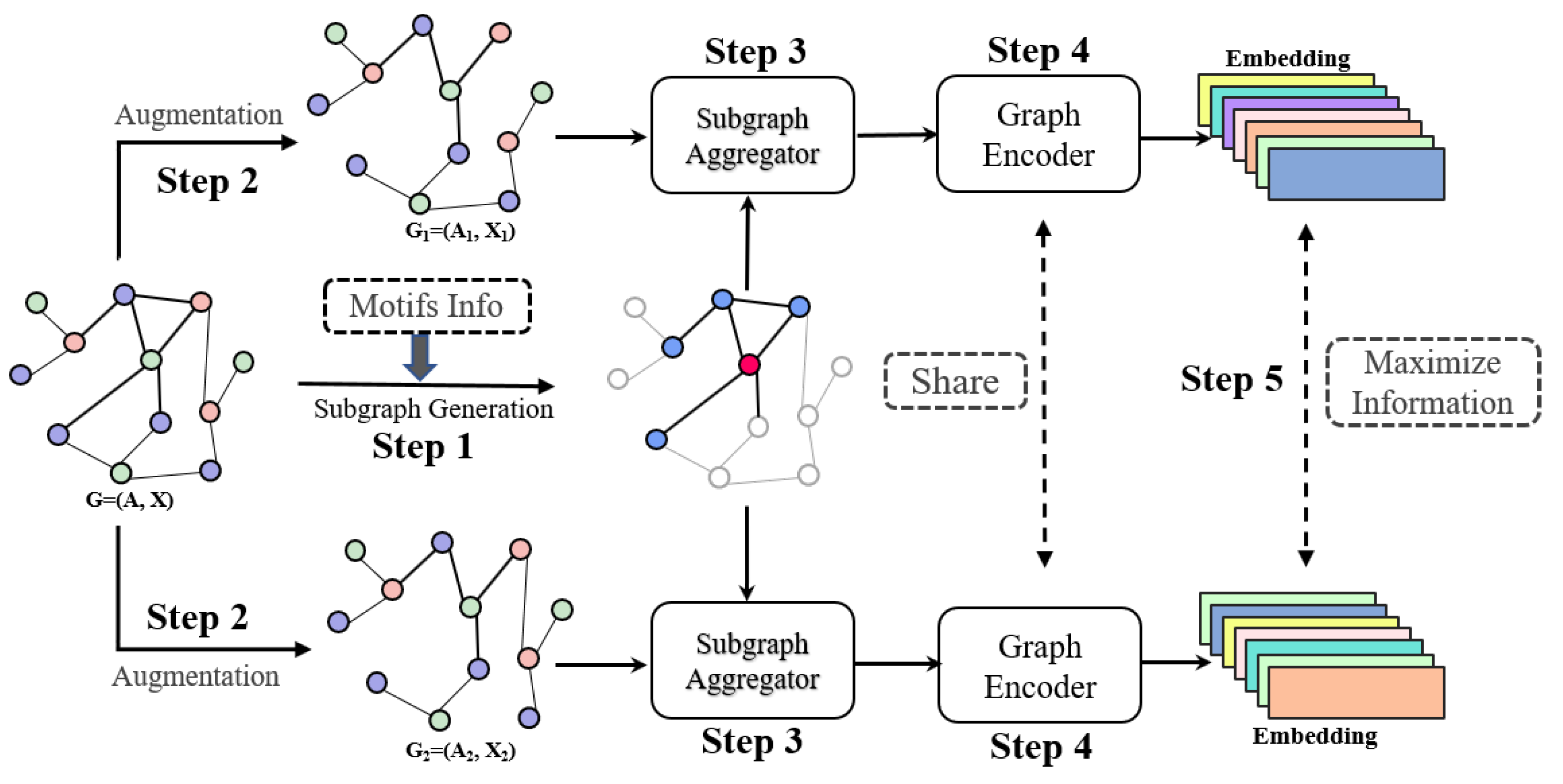
Our work. To solve the above problems, we propose a motif-based GCL method, entitled the subgraph adaptive structure-aware graph contrastive learning model (PASCAL), used for unsupervised node classification tasks in this paper. Concretely, we first adaptively extract subgraphs for each node based on its motif information to capture rich semantic information hidden in the local structure. Then, we use the feature masking and edge dropping augmentation strategies to generate two different graph views. Next, we use our proposed subgraph aggregation method to calculate subgraph embeddings. The subgraph embeddings are then regarded as node features fed to the next layer of GNNs. Finally, the graph encoder is optimized by maximizing the mutual information between the same nodes in different graph views. We conduct extensive experiments on various academic and social network datasets. Compared with previous methods, our proposed PASCAL performs better in most cases. The contributions of this work are summarized as follows:
Rich sentiment information representation. We propose an effective motif-based graph contrastive learning method, called PASCAL, for unsupervised node classification tasks. PASCAL employs motifs to formulate certain patterns containing rich sentiment information, which significantly enhances the effectiveness of graph contrastive learning.
Subgraph aggregation and encoding strategy. We propose a motif-based subgraph aggregation and encoding strategy, which is a play-and-pug component. The performance of models that imports the component can be significantly improved.
Explainable motif-aware model. To prove the reliability and interpretability of the model, we analyze the Pearson correlation coefficient between the number of motifs and learned attention weights, and the learned attention weights are in line with our intuition. Moreover, we visualize the node embeddings by t-SNE, showing that our model is explainable and trustworthy.
Excellent performance on various datasets. The effectiveness of PASCAL is shown through numerous experiments on various datasets including dblpv7, amazon-computers, etc. For the unsupervised node classification task, all methods are executed 20 times. No matter the optimal or average performance, PASCAL greatly outperforms all methods, including SOTA contrastive learning methods, under most settings.
In the following, we first introduce existing works and the preliminary of these works in
Section 2 and
Section 3, respectively. Then, we show the details of PASCAL in
Section 4.
Section 5 introduces the experimental results. The effectiveness of our proposed motif-based subgraph aggregation strategy for semi-supervised models is implemented in
Section 6. Moreover, we also analyze the learned attention weights in
Section 6, which shows that our model is explainable.
4. The Design of PASCAL
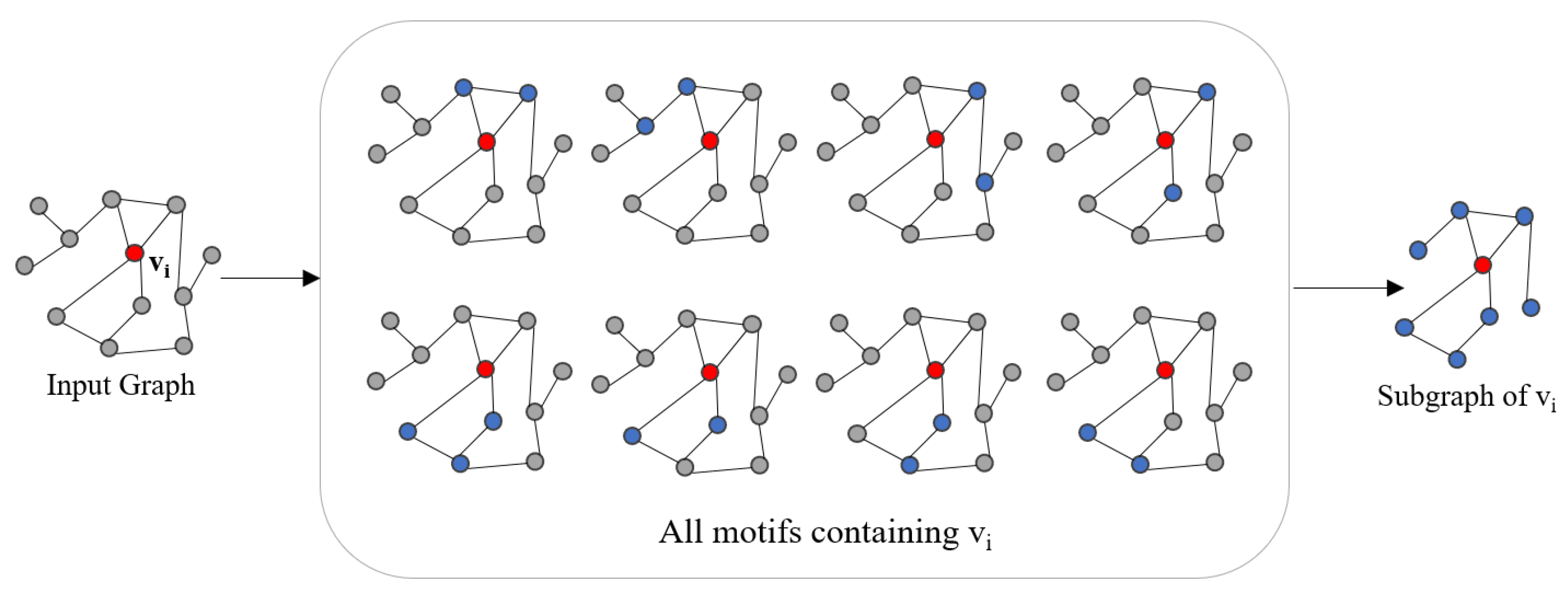
4.1. Subgraph Generator
In this work, we use pre-statistical node motif information to adaptively construct subgraphs for each node separately. As shown in
Figure 3, we first find all motifs related to target node
, denoted by
, where
represents a motif that containing
. Subsequently, we incroporate all of these motifs together as the motif-based subgraph centered on node
. The final subgraph centered on node
is represented as:
where
represents the
ith node in motifs. Algorithm 1 is the pseudocode of the subgraph construction.
| Algorithm 1 Subgraph construction. |
- Input:
Target node , the set of motifs containing the target node , node set , edge set . - 1:
form in do - 2:
Add all nodes of m to - 3:
Add all edges of m to - 4:
end for - 5:
Subgraph , where and -
Output:
Subgraph G
|
4.2. Augmentation
We use two augmentation strategies that are commonly used in GCL, feature masking and edge dropping, to generate two different graph views.
Edge Dropping. All edges of the input graph are dropped with a fixed probability. Formally, given a graph
, we first randomly sample a mask matrix
, which follows a Bernoulli distribution
if
for the input graph, or otherwise
. The
represents the probability of dropping edges. The adjacency matrix of the augmented graph is computed by Equation (
2).
where ∘ represents element-wise product.
Feature Masking. We randomly mask some dimensions of the input node features with zeros. To be specific,
represents the original feature matrix, we first randomly sample a vector
, where each dimension of it independently follows a Bernoulli distribution with probability
, i.e.,
. The feature matrixes of the two views are computed by Equation (
3).
Algothrim 2 summarizes the graph augmentation process of PASCAL.
| Algorithm 2 Graph augmentation. |
- Input:
Input graph , drop edge probability , and mask feature probability . - 1:
Construct two empty network - 2:
for to 2 do - 3:
Sample a mask matrix , where - 4:
- 5:
is the augmented feature matrix - 6:
for node v in V do - 7:
Sample a mask vector , where each dimension of it independently follows a Bernoulli distribution with probability - 8:
= , representing the augmented feature of v - 9:
end for - 10:
Augmented graph - 11:
end for - Output:
Augmented graph
|
4.3. Subgraph Aggregator
How to construct and encode subgraphs is the key to subgraph-level GCL. In this work, we design a motif-based subgraph aggregator to calculate the subgraph embeddings, which are regared as node features fed into the graph encoder. Specifically, for each node
, the motifs set containing
is represented as
, where
, and
t is the number of motif types. The subscript
j represents the different kinds of motif defined in
Section 3.3. Our proposed motif-based subgraph aggregate strategy consists of the following three steps:
- (1)
For each motif , we use a sum aggregator to compute the motif embedding, i.e., .
- (2)
After Step 1, we can obtain all motif embeddings of type j containing , denoted by . Then, we use a mean aggregator to aggregate all motif embeddings.The prototype of the j type motif containing is represented by .
- (3)
For all kinds of motif, Steps 1 and 2 are repeated. After obtaining all six kinds of motif embeddings containing , denoted by , we use an aggregator to compute the final embedding of the subgraph that centered on , denoted by .
For the function used in Step 3, a mean or attention aggregator can be used. Given the motif prototypes, where represents the number of motif types and N represents the dimension of node embeddings. The formal definitions are, respectively, shown as follows:
Mean Aggregator. The formula of
is as follows:
Attention Aggregator. We employ the attention mechanism used in UDAGCN [
40] (shown in Equation (
5)).
where
and
represent the linear and softmax function, respectively. Algorithm 3 shows the process of subgraph aggregation.
| Algorithm 3 Subgraph aggregation. |
- Input:
Pre-statistical motif information M, input graph . - 1:
represents the subgraph embedding matrix - 2:
for node v in V do - 3:
represents the motif information of v - 4:
for each type t of motifs do - 5:
represents a set of motifs of type t containing v. - 6:
Calculate each motif embedding by , i.e., - 7:
Calculate the prototype of each motif by - 8:
end for - 9:
Aggregate all motif prototypes as subgraph embedding, i.e., - 10:
end for - Output:
Subgraph embedding matrix
|
Figure 4 shows the process of calculating the triangle motif’s prototype of
. In the calculation of motif embeddings and motif prototypes, we use
and
for aggregation, respectively. Therefore, in practice, we can simplify the calculation process of subgraph embeddings to matrix multiplication.
Concretely, we define two matrices,
and
, which represent all involved nodes and the number of motif type, respectively.
represents the number of
appearing in the motif of type
t containing
. Likewise,
denotes the number of motifs of type
t containing
. The computing process of subgraph embeddings is formulated in Equation (
6).
4.4. Graph Encoder
Two graph encoders, called PASCAL-concat and PASCAL-replace, respectively, are designed.
PASCAL-concat adds an aggregation layer before message passing to compute the subgraph embedding
, which are regarded as node embeddings fed into the message passing layer. The feature update formulas for each layer of the graph encoder are as follows:
PASCAL-replace uses the subgraph aggregation to replace the original neighbor aggregation in GNN. Therefore, the adjacency matrix is useless in the graph encoder, as shown in Equation (
8).
where
is the learnable weight matrix of layer
l.
For PASCAL-concat, we use both feature masking and edge dropping augmentation strategies at the same time. However, as the adjacency matrix is not used in PASCAL-replace, only the feature masking augmentation strategy is used.
4.5. Comparator
To train a graph encoder capturing rich local semantic information in an unsupervised manner, similar to GRACE [
20], we define a contrastive objective to maximize the mutual information of the same node in two different graph views. Formally, we use
to represent our motif-based graph encoder, and
denotes the two graph views, respectively. For better comparison, we use a projection function
to map the node embeddings of the two graph views to the same contrast space. For any node
, its embeddings in two views are denoted by
and
, which are treated as the anchor and positive sample, respectively. The pairwise objective for each positive pair
is defined as Equation (
9).
where
, and
is a temperature parameter. The distance function used in
is the cosine similarity. Moreover, instead of deliberately choosing negative samples for the anchor, we treat all other nodes in the two graph views as negative samples. As two views are symmetric, the definition of
is similar to
. Therefore, the final loss of PASCAL is defined as follows:
Overall, in PASCAL, given the input graph and pre-statistical motif information, we first extract subgraphs for each node, and then perform graph augmentation to obtain different graph views and encode subgraphs based on motif information, and finally optimize the graph encoder by maximizing the mutual information between the same node in different views. The pseudocode of PASCAL is summarized in Algorithm 4.
| Algorithm 4 PASCAL-replace algorithm. |
- Input:
Input graph , motif info and , graph encoders , projection function , discriminator , loss J. and augmentation function . - 1:
for to n do - 2:
for to 2 do - 3:
= = - 4:
- 5:
for to k do - 6:
- 7:
- 8:
end for - 9:
end for - 10:
= - 11:
end for - Output:
|
6. Discussion
Complexity Analysis. Here, we briefly analyze the time complexity of PASCAL and compare it with GCN and GRACE. Let
represent the edge number in the graph;
d be the embedding size;
b and
m, respectively, denote the batch size and the node number in a batch;
denote the edge keep rate in PASCAL; and
L represent the number of layers of the encoder. We compare them from four aspects, and
Table 7 summarizes the comparison results.
Preprocessing: GCN and GRACE do not need to preprocess data, while PASCAL needs to collect the motif information of each node which is one of disadvantages of it. However, the motif information only needs to be analyzed once; the cost of preprocessing is, therefore, acceptable.
Adjacency Matrix: For GCN, the adjacency matrix has only non-zero elements since no augmentation is required. GRACE and PASCAL are typical contrastive learning methods that need to generate two augmented views, so there are two adjacency matrices containing non-zero elements.
Encoder: All three models use a two-layer encoder architecture, so the time complexity is consistent.
Loss: For GCN, the time complexity is . For GRACE and PASCAL, we only use a small amount of data to train a simple linear classifier, so the time complexity mainly depends on the contrastive loss. Both GRACE and PASCAL use other nodes in the other perspective as negative samples, so the complexity of contrastive loss is .
In general, the time complexity of contrastive learning is higher than that of GCN. Compared with GRACE, the complexity of PASCAL is higher than the additional data preprocessing. However, compared with the significant performance of PASCAL, the time cost of data preprocessing is negligible.
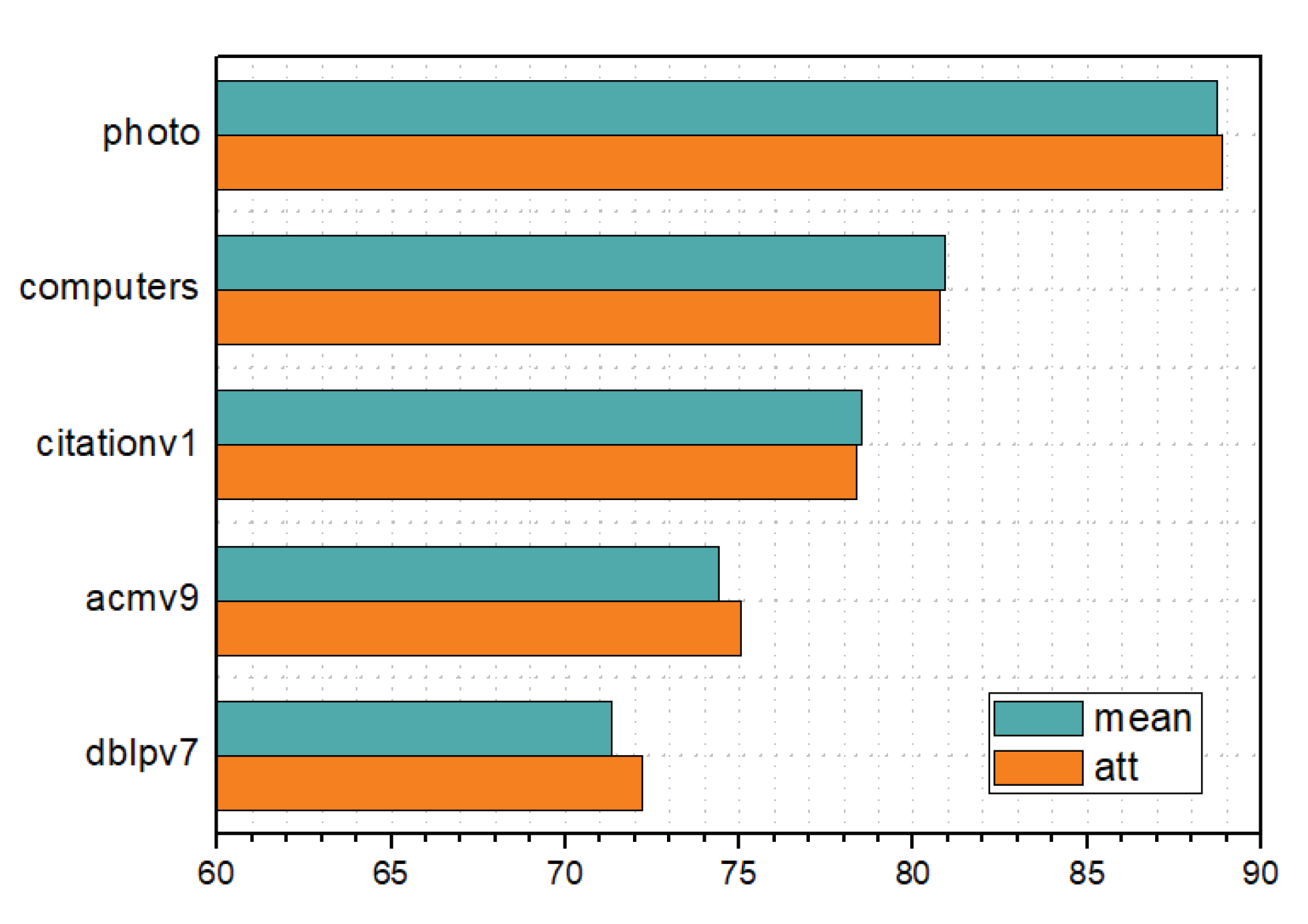
Attention weight. In the attention variant of PASCAL, we use the attention mechanism to aggregate different types of motifs. Here, we analyze the learned attention weights to explore something interesting. Specifically, we consider the relation of attention weights and the number of motifs using the Pearson correlation coefficient, which are used to measure the correlation between two variables. The results are summarized in
Table 8. From
Table 8, we can find that the number of nodes with correlation coefficients greater than 0.9 in acmv9, citationv1, and dblpv7 is much larger than that in the other three datasets, which means that the types with more motifs in the computers, photo, and polblogs may be assigned smaller weights. Actually, this phenomenon is normal. The distribution of the number of motifs in
Table 3 shows that the distribution of motifs in these three datasets is more uneven. In this case, if the correlation coefficient is large, it will overly attenuate the influence of other motifs on the model, potentially reducing model performance. Therefore, the results in
Table 8 are intuitive, indicating that the attention weights learned by the model are meaningful.
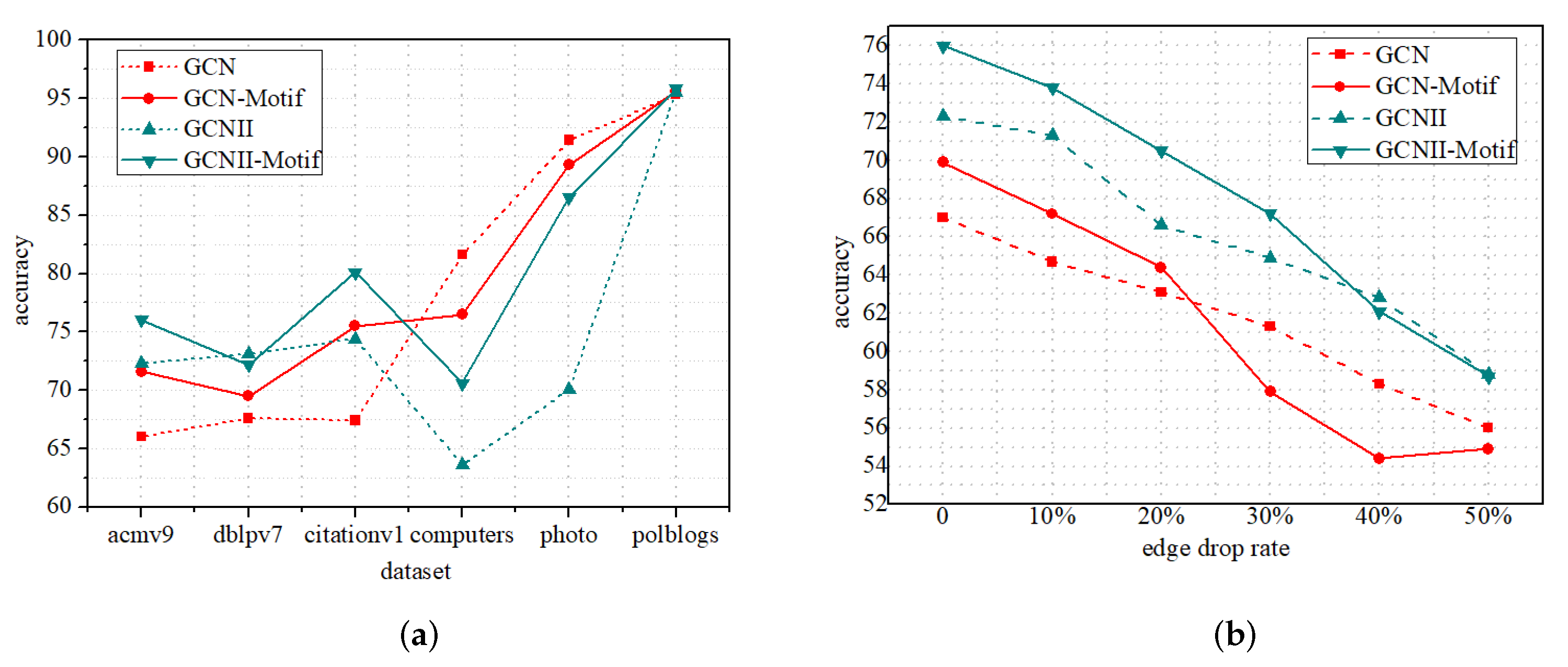
Semi-supervised node classification. To further verify the power of our proposed motif-based subgraph aggregation strategy, we integrate it into GCN and GCNII in a concat manner for semi-supervised node classification tasks. Specifically, we first perform the motif-based subgraph aggregation on the output of the previous layer. Then, it is regarded as the updated node embeddings fed into the next GNN layer.
Figure 6a,b, respectively, show the performance of the four models on the five datasets and incomplete Acmv9. From
Figure 6a, we can find that on most of the datasets, the GCN-Motif and GCNII-Motif perform better, especially GCNII-Motif, which once again verifies the effectiveness of our proposed strategy. The performance of all models degrades as the ratio of missing edges increases. When the ratio of edge dropping is low, the performance of the improved model is still better than the original model. However, when the ratio of edge loss is too large (≥30%), the performance of the improved model is comparable to or even worse than that of the original model, which is in line with our intuition. As the improved model is more dependent on the graph topology, the performance of the model will be affected more seriously if the original graph structure is excessively destroyed.
Table 9 summarizes the GCN-Motif performance under the two integration modes of replace and concat. Unlike the unsupervised framework, in the semi-supervised framework, GCN-Motif-replace and GCN-Motif-concat perform comparably, which supports our conjecture in
Section 5.2. Note that we use the Mean-Agg as the motif prototype aggregator for all experiments in this section.
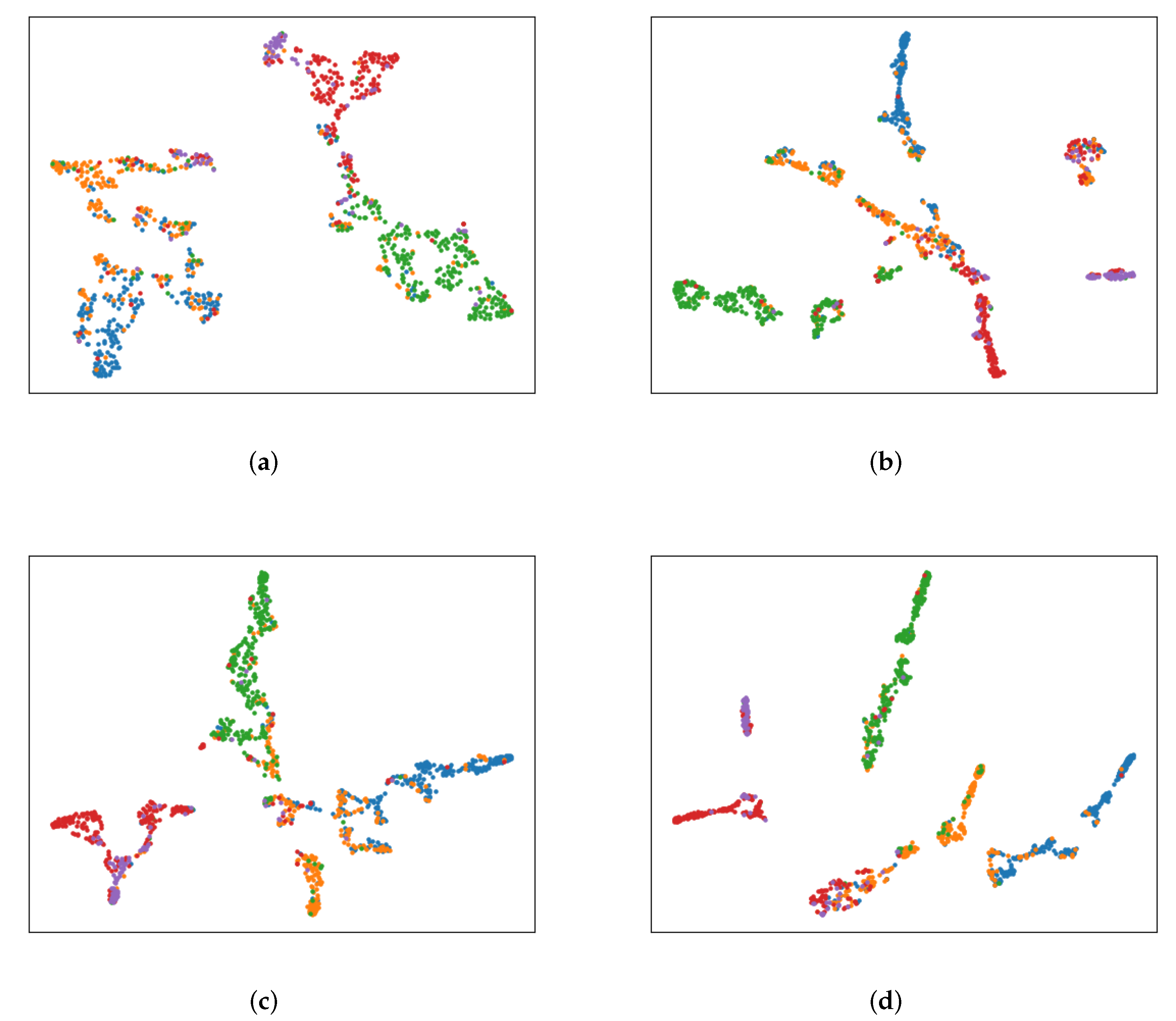
Visualization. To more intuitively show the effect of our proposed motif-based subgraph aggregation strategy on the GNNs framework, we use the tSNE algorithm to visualize the test set node embeddings learned by the model.
Figure 7a,c show the test node embeddings of GCN and GCNII on citationv1, respectively.
Figure 7b,d show the learned embeddings of GCN-Motif and GCNII-Motif, combined with our proposed subgraph strategy on citationv1. Comparing the first and second columns of
Figure 7, we find that the nodes of each category in the second column are more concentrated, and the classification boundaries are more obvious, which indicates that the quality of learned node embeddings is significantly improved through integrating our proposed subgraph strategy.
7. Conclusions
In this work, we propose a structure-aware graph contrastive learning model called PASCAL which considers the subgraph-level embedding. PASCAL adaptively constructs and encodes subgraphs based on the nodes’ motif information, and further uses them as the input of the GNN encoder to capture rich semantic information hidden in the local structure. Extensive experiments on six social and web benchmark datasets show the outperformance of PASCAL.
Although PASCAL performs well in unsupervised node classification tasks, it is not flawless. The motifs used in PASCAL are predefined, as it underperforms on some datasets such as Amazon Photo. The reason behind this phenomenon is the different distribution of motif types and numbers in different datasets. The five motifs predefined in this study may not be applicable to Amazon Photo. In future work, we will study how to automatically design and select the optimal motifs, which can significantly improve the generalization of PASCAL.


 as a special kind of motif in experiments. It is an edge in a graph, but herein we denote it as a second-order motif, so there are total six kinds of motifs used for subgraph generation and aggregation.
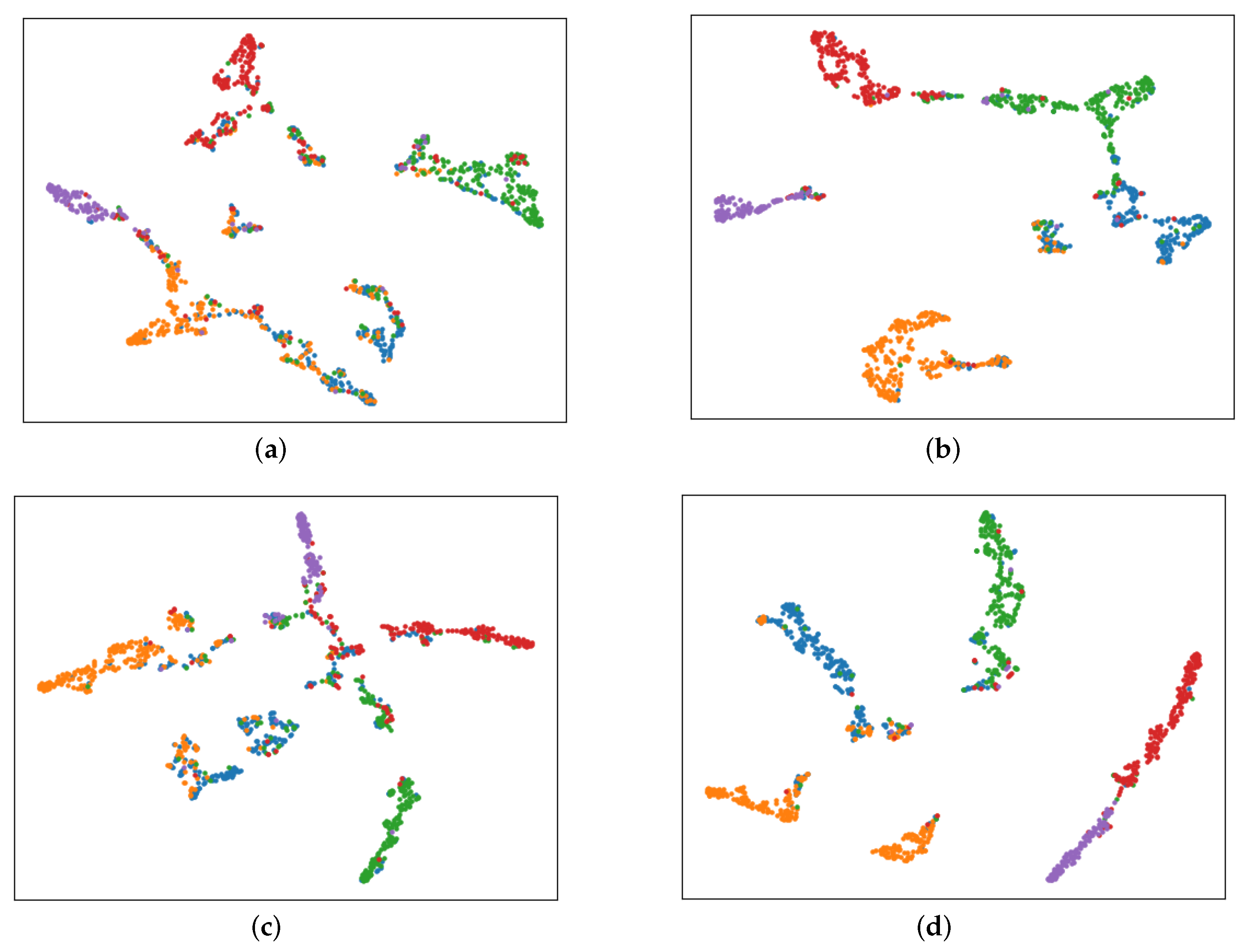


