BiInfGCN: Bilateral Information Augmentation of Graph Convolutional Networks for Recommendation

Abstract

The current graph-neural-network-based recommendation algorithm fully considers the interaction between users and items. It achieves better recommendation results, but due to a large amount of data, the interaction between users and items still suffers from the problem of data sparsity. To address this problem, we propose a method to alleviate the data sparsity problem by retaining user–item interactions while fully exploiting the association relationships between items and using side-information enhancement. We constructed a “twin-tower” model by combining a user–item training model and an item–item training model inspired by the knowledge distillation technique; the two sides of the structure learn from each other during the model training process. Comparative experiments were carried out on three publicly available datasets, using the recall and the normalized discounted cumulative gain as evaluation metrics; the results outperform existing related base algorithms. We also carried out extensive parameter sensitivity and ablation experiments to analyze the influence of various factors on the model. The problem of user–item interaction data sparsity is effectively addressed.

1. Introduction

In recent years, with the advent of the 5G era and the popularity of intelligent mobile terminals such as cell phones, the scale of online shopping has shown a continuous trend of expansion. As a result, the data generated is growing exponentially, and there is a wealth of information in this data. Therefore, it is essential for both users and merchants to quickly and effectively mine valuable information from these data. Recommendation systems are an essential tool to solve “information overload” [1,2] and have achieved good results in many fields [3,4,5,6]. Based on the user’s needs and interests, recommendation systems recommend items that may be of interest to the user from a large amount of data, such as movies [7], books [8], music [9], and so on, through the corresponding recommendation algorithms. At present, several successful applications of recommendation systems include Amazon in the field of e-commerce, Today’s Headlines in the field of information, and YouTube in the field of video browsing.

Against the backdrop of the global epidemic, more people tend to shop for what they need through e-commerce platforms. Online shopping has brought convenience to people while driving economic development. How to select items that may be of interest to people from the vast amount of information has become one of the critical challenges faced by e-commerce platforms. In recent years, breakthroughs and progress with regard to deep learning in the fields of image processing, natural language processing, and speech recognition also bring new opportunities for recommendation systems [10]. Among them, the graph neural network (GNN), which borrows ideas from the RNN and CNN, is a redefined and redesigned deep learning algorithm for processing data in non-Euclidean space.

Currently, recommendation systems based on heterogeneous graph convolution have achieved better results in the field of item recommendation, which is mainly achieved by constructing a bipartite user–item-based graph for item recommendation. For example, NGCF [11], a collaborative filtering recommendation algorithm based on graph convolution, learns the embedding representation of users and items by designing a neural network method that propagates recursively over the graph. Subsequently, LightGCN [12] further optimized and streamlined the model based on NGCF and concluded through extensive ablation experiments that using a network structure with symbolic representations of user and item nodes, feature transformations, and nonlinear activations did not contribute to the effectiveness of NGCF, but rather degraded the performance of the model. For LightGCN, the authors constructed a user–item bipartite graph for representation learning; specifically, after associating each user (item) with an ID embedding, the embedding representation is propagated on the user–item interaction graph. The embedding information from different propagation layers is then combined with a weight value to obtain the final embedding. However, more information about the user–item interactions is considered only throughout the learning process of the bipartite graph. In the whole dataset, the items that users have interacted with represent a very small percentage of the item-set, as shown in Figure 1, and the data sparsity problem is more serious, while the length distribution of the sequence of user-interaction items is very scattered. Therefore, a more available representation of user and item embeddings cannot be adequately obtained.

Because of the problem of data sparsity with regard to item recommendation, a method using side-information enhancement is proposed to deeply mine the association between items and obtain a more comprehensive and accurate user representation through each user’s historical item interaction information to be used for recommendations. The experimental results indicate that the method can better fuse the general characteristics of users and items and effectively improve the recommendation effect to users. The main contributions are as follows.

(1)

A “twin-tower” structural model with side-information enhancement is proposed. A more feature-rich user representation and item representation is obtained by use of a graph neural network and graph embedding, which can more accurately represent user preferences and characteristics of items.

(2)

In the model training process, a “mutual learning” strategy is used so that the two sides of the structure with mutually independent weights maintain higher consistency for the same sample, thus improving the expressiveness of the user and item embedding.

(3)

Related experiments were conducted on the Amazon public dataset and the Last.fm dataset and the results show that the recommendation algorithm proposed in this paper outperforms algorithms in the same category in terms of both the check-all rate and the normalized discounted cumulative gain. Notably, the model proposed in this paper has a more excellent lifting effect for data sets with higher sparsity.

2. Related Studies

The current study follows two precedents: (1) traditional recommendation algorithms and (2) recommendation algorithms based on graph convolutional neural networks.

2.1. Traditional Recommendation Algorithm

Traditional recommendation algorithms can be broadly classified into collaborative filtering-based recommendation methods [13], content-based recommendation methods [14], and hybrid recommendation methods [15]. Among them, collaborative filtering-based recommendation algorithms recommend items that users may be interested in through their historical behavior records, and they are the most classic and widely used recommendation algorithms. An example is matrix factorization [16], a method that uses the interaction information between the user and the item to make recommendations for the user. Collaborative filtering methods mainly include neighborhood-based methods and model-based methods. Neighborhood-based methods first calculate the similarity between users (or items) by the difference in users’ historical ratings and then calculate the utility value based on the historical ratings of users and the similarity between users to make recommendations. The model-based approach focuses on constructing a model of user preference to predict the user’s preference for the item. Since collaborative filtering methods only apply the user’s historical rating data, the model is simple and effective, but the recommendation accuracy is not accurate enough for cold start problems and sparsity problems. Content-based recommendation methods focus on mining other items that are similar in content to those of which users have historically interacted with in order to produce recommendations. Specifically, the process can be described as: First obtain the items that users have interacted with through explicit feedback (e.g., rating, like/dislike) or implicit feedback (e.g., clicking, searching, buying). Then, summarize and extract users’ preferences from historical items and represent them as features to calculate the matching degree between each user and the items they have not interacted with. Afterward, rank and make recommendations based on the matching degree. Content-based recommendation methods do not require a large amount of rating information and rely only on user preference features and item features. Therefore, for new items, one only need extract new-items features for a recommendation; while there is no data sparsity problem or cold start problem, there are often difficulties in extracting features. Since every single recommendation model has its own problems, a hybrid recommendation produced by combining different recommendation algorithms can often produce better recommendation results. For example, integrating content-based recommendation algorithms into a collaborative filtering framework can effectively alleviate the data sparsity problem. The hybrid recommendation algorithm models multiple recommendation algorithms and finally decides the final recommendation result by a voting method. A hybrid recommendation is theoretically no worse than any single recommendation algorithm, but at the same time increases the complexity of the algorithm.

2.2. Recommendation Algorithm Based on Graph Convolutional Neural Network

In recent years, applying deep learning to graph analysis has become a hot research topic in various fields. Bruna et al. [17] first proposed graph convolutional neural networks, defining convolution in spectral space and developing a spectral approach to the field of graph convolution; ChebNet [18] and GCN [19] parametrized the convolution kernel in the spectral approach, thus significantly reducing the spatio-temporal complexity. Graph convolutional neural networks can be divided into spectral and spatial methods. The spectral approach defines the graph convolution from the spectral domain, while the spatial approach aggregates each central node with its nearest neighbor node features by defining an aggregation function. The most widely used graph convolutional neural networks currently are spatially based graph convolutional neural networks. For example, GNNs [20] were proposed to build neural network models on graphs, in which the aggregation function was defined as a recurrent recursive function. GAT [21] adds an attention mechanism to the aggregation function, and graph attention networks use attention weights to focus the feature representations of surrounding nodes to intermediate nodes in a weighted aggregated manner. A summary of applications based on graph convolutional neural networks is shown in

Table 1. Key differences between graph deep learning models.

Application Areas	Model Name	Node
Text classification	TextGCN [29], HGAT [30], HR-DGCNN [31]	Word
User impact forecast	DeepInf [32]	User
Recommendation system	NGCF [11], LightGCN [12]	User, item
Semantic role annotation	Semantic GCN [33], C-GCN [34], LSTM + GCN [35]	Word

[22]. In the field of recommender systems, Ying et al. [23] developed a convolutional construction method based on efficient random wandering and successfully applied GCN to commercial recommender systems for the first time; the NGCF [11] model was used for user-personalized recommendation by constructing a user–item bipartite graph and employing graph convolution operations for embedding representation learning of users and items. Subsequently, He et al. [12] eliminated nonlinear operations and activation functions that were ineffective for embedding representation learning based on NGCF to reduce complexity and improve the model’s efficiency. Moreover, the development of KGCN [24] introduced knowledge graphs to recommendation systems. The main idea was to aggregate and merge biased neighborhood information when computing the representation of an entity in the knowledge graph and to capture the local neighborhood structure and store it in each entity by the operation of neighborhood aggregation. MixGCF [25] abandoned negative sampling from the raw data based on graph convolution and instead designed the hop mixing technique to synthesize hard negatives to make the training data more efficient. Since many real-life situations cannot be described using regular graphs, recommendations can be made using hypergraph convolution. UltraGCN [26] was developed with the belief that LightGCN, as a multi-layer stacking for multi-layer messaging, would affect the training efficiency and effectiveness of GCN-based recommender systems; resultantly, the loss function was constructed by setting the convergence method, thus avoiding the problems caused by multi-layer stacking. DA-GCN [27] designs a domain-aware graph convolutional network to learn the user’s representation. Moreover, two different attention mechanisms are designed for the message delivery process so that messages can be selectively delivered. Zhang et al. [28] compared the learning methods of regular graphs and hypergraphs in terms of matrix decomposition, random wandering, and deep learning and introduced the structural optimization of hypergraphs.

However, the historical interaction information between users and items only occupies a tiny portion of the overall items, so there is a data sparsity problem in using the interaction information between users and items alone for a recommendation. In this paper, we aim to alleviate the data sparsity problem and improve recommendation accuracy by fusing the association relationship between items.

This paper constructs an item relationship network based on the user–item bipartite graph. We used an appropriate network representation learning method to obtain the embedding of the item nodes. Our guiding principle was to fully explore the association relationship between items and obtain a more comprehensive item embedding representation in order to make more accurate recommendations.

3. Materials and Methods

3.1. Problem Description and Related Definitions

By introducing temporal information into the user’s interaction history, the user’s historical behavior data is transformed into time series data. The historical user behavior data with time information can be represented by a triplet $<u,i,t>$, which means that the user $u$ interacted with the item $i$ at the time $t$.

Definition 1.

Defining user interaction sequence $D=\left\{D_{u_i},u_i\in U\right\}$, where $U$ is the set of users. The sequence of user $u_i$ interactions can be denoted as $D_{u_i}=\{<u_i,i_1,t_1>,<u_i,i_2,t_2>\dots <u_i,i_k,t_k>\}$.

Definition 2.

Defining user–item bipartite graph $G_{ui}$. User interaction sequence $D$ is known, construct a user–item bipartite graph $G_{ui}=\left(V_{ui},E_{ui}\right)$, where the set of nodes $V_{ui}=\left\{U{\displaystyle \cup I}\right\}$ contains the set of users $U=\left\{u\right\}$ and the set of items $I=\left\{i\right\}$. The edges $E_{ui}$ indicate the existence of interaction between user and item.

Definition 3.

Defining item–item homogeneous network $G_{ii}$. User interaction sequence $D$ is known, construct an item–item network $G_{ii}=\left(V_{ii},E_{ii}\right)$, where $V_{ii}=\left\{I\right\}$ denotes the set of items. If the historical interaction item $i_1$ and item $i_2$ of user $u\left(u\in U\right)$ are adjacent in the interaction series and the interaction time difference complies with $\Delta t=|t_2-t_1|<\partial$, then establish an edge relationship between the item $i_1$ and the item $i_2$, and the last edges set denoted as $E_{ii}$.

3.2. Model Structure

According to Definition 2, the simple user–item bipartite graph has intense data scarcity, which leads to inaccurate recommendation results. Therefore, we propose our model, BiInfGCN. By building a “twin-tower” structure with independent weights for a user–item bipartite graph and an item–item homogeneous network, a more comprehensive representation of user and item characteristics can be obtained, thus improving the accuracy of recommendations. The model is shown in Figure 2.

3.2.1. Graph Construction and Embedding Propagation

In the BiInfGCN model, the left-hand side is a graph convolution structure based on the user–item bipartite graph, which mainly contains a bipartite graph construction layer, initial embedding layer, and embedding propagation layer. First, according to Definition 2, a user–item bipartite graph is constructed based on the interaction between users and items. Then, the initial embeddings of user and item are obtained by the initial embedding layer. The GCN-like propagation architecture is constructed in the embedding propagation layer, and the graph convolution operation is performed by an iterative method so that each node eventually aggregates the features of its neighbor nodes. The user node aggregation is shown in Equation (1). Specifically, taking the user node $u$ as an example, the node $u$ in the $k+1$ layer of the graph convolution aggregates the features of the neighboring nodes in the $k$ layer. Similarly, the item node $i$ in the $k+1$ layer aggregates the features of the neighboring nodes in the $k$ layer, and the aggregation is shown in Equation (2).

$$e_u^{(k+1)}={\displaystyle \sum _{i\in N_u}\frac{1}{\sqrt{\left|N_u\right|}\sqrt{\left|N_i\right|}}}{e}_i^{(k)}$$

(1)

$$e_i^{(k+1)}={\displaystyle \sum _{u\in N_i}\frac{1}{\sqrt{\left|N_i\right|}\sqrt{\left|N_u\right|}}}{e}_u^{(k)}$$

(2)

During the aggregation process, a symmetric normalization term is added, which is in accordance with standard GCN design and can effectively prevent the excessive increase of embedding size during graph convolution. The final user (item) embedding representation uses the right-value sum of the embeddings of each convolutional layer, as shown in Equations (3) and (4):

$$e_u={\displaystyle \sum _{k=0}^K{\partial }_k{e}_u^{(k)}}$$

(3)

$$e_i={\displaystyle \sum _{k=0}^K{\partial }_k{e}_i^{(k)}}$$

(4)

where K denotes the number of convolutional layers and the weight-value parameter for each convolutional layer is adjustable. The final embeddings of users and items obtained from the “left tower” structure are denoted as $E_u^l=[e_{u_1}^l,e_{u_2}^l,\cdots ,e_{u_N}^l]$, $E_i^l=[e_{i_1}^l,e_{i_2}^l,\cdots ,e_{i_M}^l]$, respectively. The loss function loss_left is calculated from the user and item embeddings obtained from the “left tower” structure as shown in Equation (5). $y_{u^l{i}^{l+}}$ and $y_{u^l{i}^{l-}}$ are defined as the inner product of user and item final representations, such as ${\stackrel{⌢}{y}}_{ui}=e_u^T{e}_i$.

$$los{s}_{left}={\displaystyle \sum _{(u^l,i^{l+},i^{l-})\in D_l}-[\ln \sigma (y_{u^l{i}^{l+}}-y_{u^l{i}^{l-}})]}$$

(5)

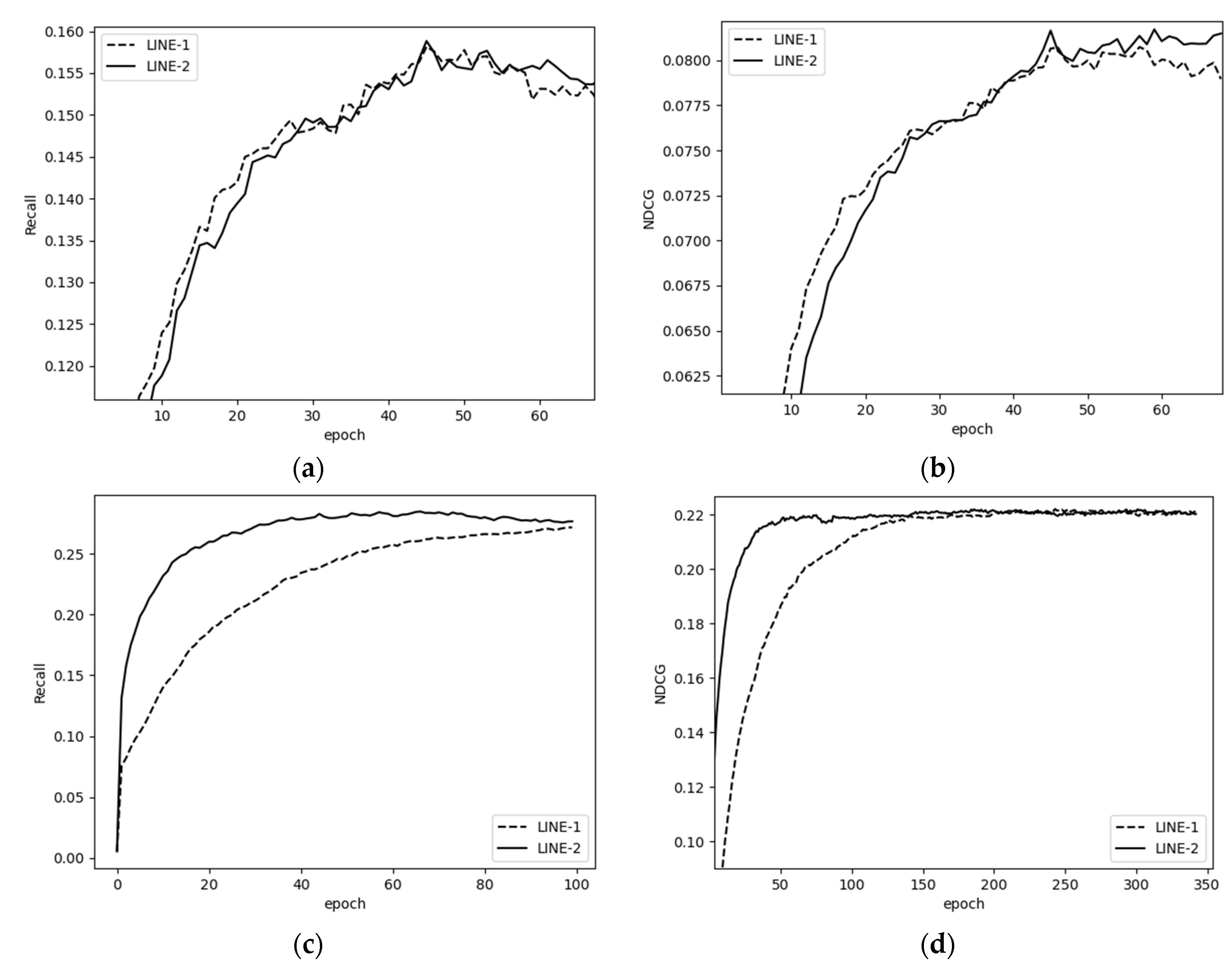
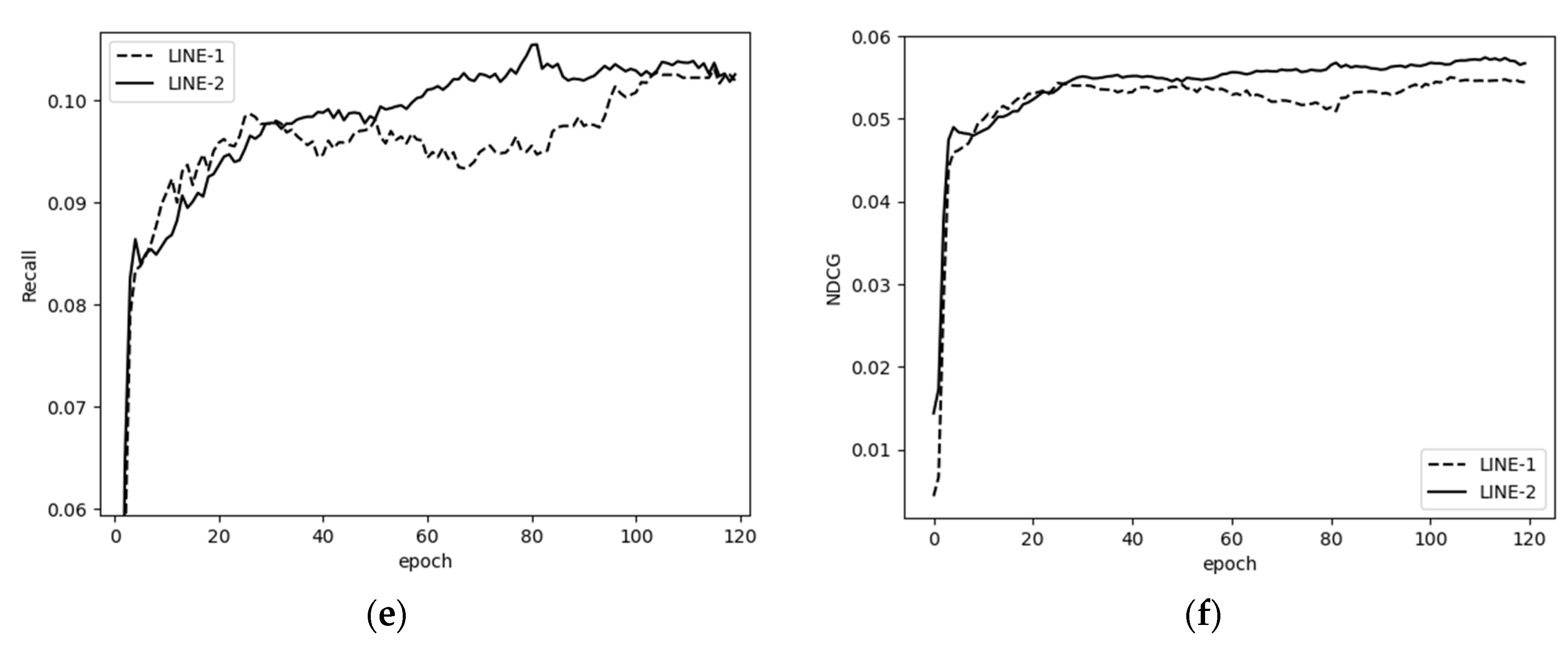
The right side shows the graph embedding structure based on an item–item homomorphic network. It mainly includes a homogeneous graph construction layer and a graph embedding representation layer. First, according to Definition 3, the item–item isomorphic graph is constructed, and then the final items’ embeddings are obtained by using the graph embedding layer. We used two approaches to learn the information network embedding, which are referred to as LINE 1 and LINE 2 in the following.

• LINE 1: First-order similarity method.

If two item nodes in the network are directly connected, then it indicates that the node pair is more closely related and should have high similarity.

First-order similarity mainly characterizes the local similarity structure in the network. Supposing there exists an edge between item nodes $i_1$ and $i_2$, and the embeddings of $i_1$ and $i_2$ are $e_{i_1}$ and $e_{i_2}$, respectively, define the co-occurrence probability between the two as shown in Equation (6), and the empirical distribution between the two exists as shown in Equation (7):

$$p_1(i_1,i_2)=\frac{1}{1+\exp (-{\overrightarrow{e}}_{i_1}\cdot {\overrightarrow{e}}_{i_2})}$$

(6)

$${\stackrel{⌢}{p}}_1(i_1,i_2)=\frac{w_{i_1{i}_2}}{W}$$

(7)

where $w_{i_1,i_2}$ denotes the weight of edge $e=(i_1,i_2)$ and $W$ is the sum of the weights of all edges. The goal is to make the co-occurrence probability as close as possible to the empirical distribution, i.e., to minimize Equation (8).

$$O_1=d({\stackrel{⌢}{p}}_1,p_1)$$

(8)

$d$ denotes the distance between the two distributions. Further, by introducing KL scatter, Equation (8) can be reduced to Equation (9). Finally, model training by minimizing the objective Equation (9) can lead to a low-dimensional dense embedding representation of item nodes.

$$O_1=-{\displaystyle \sum _{(1,2)\in E}{w}_{12}\log p_1(i_1,i_2)}$$

(9)

• LINE 2: Second-order similarity method.

When the item–item network is constructed, the relationship between two nodes directly connected is certainly close, but it fails to fully reflect the structural information of the network. Here, the neighbors of the nodes are taken as the context information of the current node, and the relationship between two nodes is closer assuming that there are more common neighbors, i.e., two nodes have more similar context information. On this basis, the second-order similarity aggregates both the neighboring node information and the structural information of the node when calculating the node embedding representation. In second-order similarity, each node acts as a central node and also as a context node for other central nodes. Therefore, there exists a central vector representation and a context vector representation for each item node. Suppose there exists an edge e between item nodes $i_1,i_2$. The embedding of $i_1$ as the central node is $e_{i_1}$ and the embedding of $i_2$ as the contextual node is $e_{i_2}^{\prime }$. Define the probability of generating context node $i_2$ with $i_1$ as the central node as shown in Equation (10):

$$p_2(i_2|i_1)=\frac{\exp ({\overrightarrow{e}}_{i_2}^{\prime }{}^T\cdot {\overrightarrow{e}}_{i_1})}{{\displaystyle {\sum }_{k=1}^{\left|V\right|}\exp ({\overrightarrow{e}}_{i_k}^{\prime }{}^T\cdot {\overrightarrow{e}}_{i_1})}}$$

(10)

where |V| denotes the number of nodes in the network. The conditional of the distribution with node $i_1$ as the central node can be expressed as $p_2(\cdot |i_1)$. Meanwhile, there exist empirical distribution probabilities as shown in Equation (11):

$${\stackrel{⌢}{p}}_2(i_2|i_1)=\frac{w_{i_1{i}_2}}{d_{i_1}}=\frac{w_{i_1{i}_2}}{{\displaystyle \sum _{k\in N(i_1)}{w}_{i_1{i}_k}}}$$

(11)

where $w_{i_1{i}_2}$ is the weight of edge $e=(i_1,i_2)$ and $N(i_1)$ denotes the set of its contextual nodes when $i_1$ is the central node, i.e., the set of neighboring nodes of node $i_1$. Therefore, the empirical distribution with node $i_1$ as the central node can be expressed as $\widehat{p_2}(\cdot |i_1)$. Again, the goal is to make the conditional distribution approximate the empirical distribution and introduce KL scatter to characterize the distance between the conditional and empirical distributions. We use the degree $d_{i_1}$ of a node to denote the weight of that node in the network. We can obtain the objective function as shown in Equation (12).

$$O_2={\displaystyle \sum _{j\in V}{d}_j{D}_{KL}({\widehat{p}}_2(\cdot |i_j),p_2(\cdot |i_j))}$$

(12)

Equation (13) is obtained by eliminating non-influential parameter simplification. We can arrive at a low-dimensional dense item node embedding representation by minimizing the objective function (13).

$$O_2=-{\displaystyle \sum _{(i_1,i_2)\in E}{w}_{i_1{i}_2}\log p_2(i_2|i_1)}$$

(13)

By LINE I or LINE II, we can obtain the item embedding matrix of the “right tower” structure, denoted as $E_i^r=[e_{i_1}^r,e_{i_2}^r,\cdots ,e_{i_M}^r]$.

3.2.2. Obtain Embedded Representations and Score Predictions

Combining the item embedding representation $E_i^r$ obtained from the right tower’s embedding representation layer with each user’s historical interaction sequence for the item yields the user’s embedding representation, as shown in Equation (14):

$${\overrightarrow{e}}_u^r={\displaystyle \sum _{i\in S(u)}{\overrightarrow{e}}_i^r}$$

(14)

where $S(u)$ denotes the set of historical interaction items of user $u$.

Finally, the embeddings of users and goods are obtained from the “right tower” structure, denoted as $E_u^r=[e_{u_1}^r,e_{u_2}^r,\cdots ,e_{u_N}^r]$, $E_i^r=[e_{i_1}^r,e_{i_2}^r,\cdots ,e_{i_M}^r]$, respectively. The loss function $los{s}_{right}$ is calculated from the user and item embeddings obtained from the “right tower” structure as shown in Equation (15).

$$los{s}_{right}={\displaystyle \sum _{(u^r,i^{r+},i^{r-})\in D_r}-[\ln \sigma (y_{u^r{i}^{r+}}-y_{u^r{i}^{r-}})]}$$

(15)

The bottom layer of the “twin tower” structure is the embedding connection layer and the recommendation prediction layer. The embedding connection layer concatenates the user embedding and the item embedding obtained from the “left tower” and the “right tower” to obtain the final embedding matrix representation, as shown in Equations (16) and (17).

$$E_u=E_u^l\oplus E_u^r=[e_{u_1},e_{u_2},e_{u_3}\dots e_{u_N}]$$

(16)

$$E_i=E_i^l\oplus E_i^r=[e_{i_1},e_{i_2},e_{i_3}\dots e_{i_M}]$$

(17)

The score prediction layer calculates the similarity score between users and items as shown in Equation (18) and makes recommendations to users based on high score. Afterward, we select the items with top k-ratings as the items that users are most likely to interact with next in order to achieve the effect of personalized recommendation.

$$Score(u_i,i_j)=e_{u_i}\otimes e_{i_j},(e_{u_i}\in E_u,e_{i_j}\in E_i)$$

(18)

3.2.3. Model Optimization

The experiments used Bayesian personalized ranking (BPR) loss, which is widely used in recommender systems [36]; this loss function was a personalized ranking algorithm based on Bayesian posterior optimization. The core aim was to personalize the recommendation by modeling the user’s preferences, calculating the items of potential interest to the user, and selecting the items from which the user has not interacted for ranking. The BPR loss function is calculated as shown in Equation (19):

$$Los{s}_{BPR}=\raisebox{1ex}{${\displaystyle \sum _{u,i^{+},i^{-}\in D}}{\displaystyle \sum _{(u^l,i^{l+},i^{l_{-}})\in D_l}}{\displaystyle \sum _{(u^r,i^{r+},i^{r_{-}})\in D_r}}-[\ln \sigma (y_{u{i}^{+}}-y_{u{i}^{-}})+\ln \sigma (y_{u^l{i}^{l+}}-y_{u^r{i}^{r+}})]+los{s}_{right}+los{s}_{left}$}\!\left/ \!\raisebox{-1ex}{$4$}\right.+\lambda ||\Theta |{|}^2$$

(19)

where $D_l$ denotes the set of positive and negative user–item pairs obtained from the “left tower” structure. Similarly, $D_r$ denotes the set of user–item positive and negative sample pairs obtained from the “right tower” structure. $D$ denotes the final set of user–item positive and negative sample pairs. The $los{s}_{l-r}=\ln \sigma (y_{u^l{u}^{l+}}-y_{u^r{u}^{r+}})$ loss function makes both sides of the structure (“left tower” and “right tower”) learn from each other during the back-propagation process. $\sigma$ denotes the Sigmoid function. $\lambda \left|\right|\Theta |{|}^2$ is the canonical term, where $\lambda$ is a tunable parameter and ${\Vert \cdot \Vert }^2$ is a two-parameter number to prevent overfitting by adjusting the parameter size. $\Theta$ is actually the initial representation vector of users and items in this loss function, i.e., $\Theta =\{E_u^0+E_i^0\}$, and $(e_{u_0}^0,e_{u_1}^0,\cdots ,e_{u_N}^0)\in E_u^0$, $(e_{i_0}^0,e_{i_1}^0,\cdots ,e_{i_M}^0)\in E_i^0$. Therefore, the trainable parameters in this model are the initial vector representations of users and items, and the model is optimized using stochastic gradient descent. The experiments used the control variable method to train the model by adjusting the main parameters, and after several experiments, the main parameters were set as shown in

Table 2. Model parameter table.

Parameter Name	Parameter Description	Parameter Value
$los{s}_l$	“Left tower” structure loss rate	0.0003
$los{s}_r$	“Right tower” structure loss rate	0.1
Layer	Number of iterations of the “left tower” structure	4
Dim	Dimension	128
Λ	L2 regularization parameter	1 × 10−4
Batch	Test set batch size	100

. The BiInfGCN model can achieve the best results under comprehensive conditions.

4. Results

4.1. Data Set and Evaluation Indicators

The more widely used Amazon dataset and the Last.fm music dataset were used for this experiment. The Amazon dataset used video-partitioned goods and automotive-partitioned goods. All of the above datasets included user ID, item ID, and interaction timestamp information. For each user, the purchased items were sorted by time, with the first 80% of the time as the training set and the last 20% as the test set. The statistical results of the dataset are shown in

Table 3. Data set statistics table.

Dataset	Number of Users	Number of Items	Number of Interactions	Density
Video	5130	1685	37,126	0.004295
Automotive	2928	1835	20,473	0.00381
Last.fm	1880	4489	52,668	0.006201

.

4.2. Comparison Models and Indicators

(a) LFM [37] (latent factor model) is a classical matrix decomposition algorithm that is an implicit semantic model algorithm. According to the user’s interaction behavior such as clicking or not clicking on the item, LFM retrieves the relationship between the user and the item and makes a recommendation by judging the attention relationship between the user and the item. Since this algorithm needs to traverse the graph structure, it has the problem of low efficiency, and the sparsity and complexity of the real data set also affects the performance of this algorithm.

(b) NGCF is a collaborative filtering algorithm on graph structure that applies the GCN model to recommender systems to obtain the embedded representations of users and items and calculates the relationship scores between them for prediction by using the user–item bipartite graph.

(c) Light-GCN is based on NGCF, and it was developed with the belief that the feature transformations and nonlinear activation functions in the NGCF model have no practical effect on collaborative filtering, instead increasing the complexity of the model while reducing the recommendation effect. Therefore, Light-GCN only adopts the neighborhood aggregation method for iteration. The experimental results show that the recommendation effect of Light-GCN is significantly improved.

(d) UltraGCN takes into consideration that the iterative layers in LightGCN can be omitted, so the model is further simplified, and the loss function is added to improve the recommendation effect.

The evaluation metrics used in this paper are the check-all rate (Recall@k) and the normalized discounted cumulative gain (NDCG@k). The experimental results are given in percentages. In this experiment, k was uniformly set to 20. Recall@k represents the ratio of the number of items with real user interactions to the number of items with user interactions in the test set in the given recommendation list of length k. Therefore, the higher the completion rate, the better the recommendation effect. The formula for calculating the full rate is shown in Equation (20):

$$Recall@k=\frac{{\displaystyle {\sum }_{u\in U}|R(u)\cap T(u)|}}{{\displaystyle {\sum }_{u\in U}|T(u)|}}$$

(20)

where $R(u)$ denotes the list of recommendations made to user $u$ and its length is 20. $T(u)$ denotes the list of items that user $u$ has interacted with in the test set. NDCG@k is used to evaluate the recommended list, which is calculated as shown in Equation (21).

$$NDCG@k=\frac{DCG@k}{IDCG@k}=\frac{{\displaystyle \sum _{i=1}^k\frac{re{l}_i}{{\log }_2(i+1)}}}{{\displaystyle \sum _{i=1}^{\left|REL\right|}\frac{re{l}_i}{{\log }_2(i+1)}}}$$

(21)

$re{l}_i$ denotes the authenticity-related score of the $i-th$ result in the recommendation list. Since the recommendation list is sorted according to the similarity score, the higher the similarity with the user, the higher the ranking of the item. NDCG@k determines the quality of the recommendation list based on the user’s real history of interacting with the item.

4.3. Experimental Results and Analysis

In this paper, extensive parameter sensitivity experiments are conducted and analyzed. By adjusting the embedding dimension of the “right tower” structure, the evaluation index values were calculated for node embedding dimensions of d = 16, 32, 64, 128, and 256, and the results are shown in

Table 4. Comparison of experimental results in different dimensions.

Dimension		16	32	64	128	256
Video	Recall	15.405507	15.54806	15.628977	15.963539	15.592613
	NDCG	8.04577	8.11645	8.14968	8.350085	8.14689
Last.fm	Recall	27.24471	27.5966	28.05809	28.54347	27.98139
	NDCG	20.86728	21.542451	21.76676	22.51918	21.664506
Automotive	Recall	9.366868	9.571416	9.771418	10.5495	9.139674
	NDCG	4.937601	5.214604	5.282281	5.49125	5.034705

Bolded numbers indicate the best results of the experiment.

.

It is observed that both Recall@20 and NDCG@20 improve to different degrees as the dimensionality increases. However, the effect decreases when the dimensionality increases from 128 to 256, with the most significant decrease in the automotive dataset. To analyze the reason, due to the different sparsity of different datasets, embeddings of different dimensions were used to represent user and item nodes in different effects. Therefore, the negative effect of overfitting occurred when a lower sparse dataset learned a high-dimensional embedding representation, which led to an excessive reduction of evaluation metrics. The results of the Last.fm dataset are also presented visually in Figure 3 so that the degree of change of the evaluation indicators as dimensionality increases can be observed more intuitively.

The effect improvement is more apparent when the low dimension is increased, and the effect improvement is relatively slow when the dimension is increased from 64 to 128.

In order to verify the relationship between the model and the number of training layers, the “left tower” structure was set as 1–5 layers for experiments, and the experimental results are shown in

Table 5. Iterative layer comparison test results.

Layer		1	2	3	4	5
Video	Recall	14.78157	15.383259	15.592613	15.963539	15.973481
	NDCG	7.557849	7.927225	7.991041	8.350085	8.3550
Last.fm	Recall	27.14997	28.044526	28.468092	28.54347	28.54421
	NDCG	20.720242	21.509124	21.944728	22.51918	22.52936
Automotive	Recall	7.47129	8.945426	9.656771	10.5495	10.449521
	NDCG	4.011684	4.883305	5.111121	5.49125	5.49013

Bolded numbers indicate the best results of the experiment.

.

Table 5 shows that the model’s performance improved as the number of iteration layers increased. In particular, the performance improvement was most significant when the number of iterations increased from one to two. However, in the subsequent iterations, the performance improvement was slower as the number of model layers increased. The reason for this is that when the number of iteration layers is 1, each user node only aggregates the features of historically interacted-with items, i.e., first-order neighbors, and cannot fully explore the close relationships between similar users. Therefore, the nodes can learn more information by increasing the number of iteration layers.

In contrast, the evaluation metrics of the automotive dataset decreased when the number of iteration layers reached 5. This is because the automotive dataset was too sparse, and overfitting occurs when the number of iteration layers is too deep. Therefore, considering the model’s time complexity and performance, a 4-layer model was chosen for the experiments.

For the “right tower” structure, the first-order and second-order similarities were used for comparison experiments, and the results are shown in

Table 6. The experimental results of first-order similarity and second-order similarity.

Model		LINE-1	LINE-2
Video	Recall	15.815764	15.963539
	NDCG	8.065501	8.350085
Last.fm	Recall	28.224349	28.54347
	NDCG	22.539373	22.51918
Automotive	Recall	10.2309778	10.5495
	NDCG	5.477437	5.49125

Bolded numbers indicate the best results of the experiment.

below.

As seen in Table 6, for both the video and the automotive datasets, the second-order similarity model Recall values and NDCG values are slightly higher than the first-order similarity model. On the Last.fm dataset, the Recall value of the second-order similarity model is higher than that of the first-order similarity model. On the other hand, the NDCG value is slightly lower than that of the first-order similarity model. By visualizing the two evaluation metrics of each dataset in Figure 4, the difference between the final effects of the two models is not too significant. However, the second-order similarity model converges faster, as shown in Figure 4c,d on the Last.fm dataset. Based on the above analysis, the model structure of second-order similarity was used in this experiment.

The experimental results in

Table 7. Experimental results of different models under 3 public datasets.

Model		LFM	NGCF	Light-GCN	UltraGCN	BiInfGCN	Improve (%)
Video	Recall	12.692095	11.568	15.04462	14.4278	15.963539	6.1
	NDCG	6.746628	5.566	7.742759	7.67025	8.350085	7.84
Last.fm	Recall	17.727586	24.518	27.9957	28.0023	28.54347	1.932
	NDCG	12.780049	18.659	22.17957	22.2137	22.51918	1.375
Automotive	Recall	5.835464	7.9051	9.8707	9.8247	10.5495	6.88
	NDCG	3.032367	5.0963	5.2786	5.1428	5.49125	4.03

Bolded numbers indicate the best results of the experiment.

show that on the publicly available datasets for videos, Last.fm, and automotives, this paper’s model, BiInfGCN, scored higher than the three benchmark models in the evaluation metrics Recall@20 and NDCG@20, with scores at least 1.932% higher in Recall@20 and at least 1.375% higher in NDCG@20. The experimental results demonstrate the validity of the BiInfGCN model. For the BiInfGCN model proposed in this paper, the node vector representation was randomly initialized, and the stochastic gradient descent algorithm was used to optimize the model. Meanwhile, to ensure the stability and accuracy of the experimental results, ten runs were conducted for this model experiment and the comparison experiment, and the average value was taken as the final evaluation basis.

5. Discussion

Based on the fact that most of the current recommendation algorithm datasets suffer from the sparsity problem of too little user–item interaction data or a significant gap in the length of interaction sequences, this paper proposes to dig deeper into the association relationships between items by building an item–item network, and subsequently more accurate extraction of user preference information for items, thus improving recommendation accuracy. Secondly, for the “twin-tower” structural model proposed in this paper, we introduced the difference between the positive sample scores of the left structure and the positive sample scores of the right structure into the BPR loss function so that the left and right models could effectively learn from each other in the process of backpropagation. Finally, extensive comparison experiments were conducted on the public Amazon and Last.fm datasets. The results show that the recommendation model proposed in this paper helps improve the recommendation effect.

As can be seen from Table 3, the sparsity of the three datasets is ranked from high to low as automotive, video, Last.fm. According to Table 7, we can see the most noticeable improvement of recommendation effect in the automotive dataset and video dataset; the improvement in Recall reached more than 6%, while the improvement in NDCG reached 4.03% and 7.84%. In contrast, the Recall and NDCG of the Last.fm dataset only improved by 1.932% and 1.375%. This shows that the BiInfGCN model significantly improved the more intensely sparse dataset, while the improvement for the weakly sparse dataset was average. Therefore, it is well demonstrated that the BiInfGCN model can effectively solve the problem of poor recommendation caused by data sparsity.

6. Conclusions

The BiInfGCN model effectively solves or alleviates the problem of unsatisfactory recommendation results caused by data sparsity. For example, fewer shopping or interaction records exist for users who have just registered on the e-commerce platform, and this model can effectively make accurate recommendations for users. However, this model still has room for improvement. According to the actual situation, there is a specific relationship between user preferences and time. Users may be more interested in recently browsed or interacted items; that is to say, recently interacted items can better reflect the user’s preferences and thus be more meaningful for a recommendation. The user embedding representation of the “right tower” of the BiInfGCN model uses the mean value of the embedding representation of the interacting items. It does not differentiate between all interacting items based on time nodes. Therefore, we will focus on this point for the following study.

References

1. Yao, J. A Review of Personalized Recommender Systems. China Collect. Econ. 2020, 25, 71–72. [Google Scholar]
2. Warren, J.; Marz, N. Big Data: Principles and Best Practices of Scalable Realtime Data Systems; Simon and Schuster: New York, NY, USA, 2015. [Google Scholar]
3. Carrer-Neto, W.; Hernández-Alcaraz, M.L.; Valencia-García, R.; García-Sánchez, F. Social Knowledge-Based Recommender System. Application to the movies domain. Expert Syst. Appl. 2012, 39, 10990–11000. [Google Scholar] [CrossRef]
4. Winoto, P.; Tang, T.Y. The Role of User Mood in Movie Recommendations. Expert Syst. Appl. 2010, 37, 6086–6092. [Google Scholar] [CrossRef]
5. Lee, S.K.; Cho, Y.H.; Kim, S.H. Collaborative Filtering with Ordinal Scale-Based Implicit Ratings for Mobile Music Recommendations. Inf. Sci. 2010, 180, 2142–2155. [Google Scholar] [CrossRef]
6. Núñez-Valdéz, E.R.; Lovelle, J.M.C.; Martínez, O.S.; García-Díaza, V.; de Pablos, P.O.; Marín, C.E.M. Implicit Feedback Techniques on Recommender Systems Applied to Electronic Books. Comput. Hum. Behav. 2012, 28, 1186–1193. [Google Scholar] [CrossRef]
7. An, H.; Kim, D.; Lee, K.; Moon, N. MovieDIRec: Drafted-Input-Based Recommendation System for Movies. Appl. Sci. 2021, 11, 10412. [Google Scholar] [CrossRef]
8. Ekstrand, M.D.; Kluver, D. Exploring Author Gender in Book Rating and Recommendation. User Modeling User-Adapt. Interact. 2021, 31, 377–420. [Google Scholar] [CrossRef]
9. Wen, X. Using Deep Learning Approach and IoT Architecture to Build the Intelligent Music Recommendation System. Soft Comput. 2021, 25, 3087–3096. [Google Scholar] [CrossRef]
10. Huang, L.; Jiang, B.; Lv, S. Survey on Deep Learning Based Recommender Systems. Chin. J. Comput. 2018, 41, 1619–1647. [Google Scholar]
11. Wang, X.; He, X.; Wang, M.; Feng, F.; Chua, T.S. Neural Graph Collaborative Filtering. In Proceedings of the 42nd international ACM SIGIR Conference on Research and Development in Information Retrieval, Paris, France, 21–25 July 2019; pp. 165–174. [Google Scholar]
12. He, X.; Deng, K.; Wang, X.; Li, Y.; Zhang, Y.; Wang, M. Lightgcn: Simplifying and Powering Graph Convolution Network for Recommendation. In Proceedings of the 43rd International ACM SIGIR Conference on Research and Development in Information Retrieval, Xi’an, China, 25–30 July 2020; pp. 639–648. [Google Scholar]
13. Mooney, R.J.; Roy, L. Content-Based Book Recommending Using Learning for Text Categorization. In Proceedings of the fifth ACM Conference on Digital Libraries, San Antonio, TX, USA, 2–7 June 2000; pp. 195–204. [Google Scholar]
14. Breese, J.S.; Heckerman, D.; Kadie, C. Empirical Analysis of Predictive Algorithms for Collaborative Filtering. arXiv 2013, arXiv:13017363. [Google Scholar]
15. Balabanović, M.; Shoham, Y. Fab: Content-Based, Collaborative Recommendation. Commun. ACM 1997, 40, 66–72. [Google Scholar] [CrossRef]
16. Lee, D.D.; Seung, H.S. Learning the Parts of Objects by Non-Negative Matrix Factorization. Nature 1999, 401, 788–791. [Google Scholar] [CrossRef] [PubMed]
17. Bruna, J.; Zaremba, W.; Szlam, A.; LeCun, Y. Spectral Networks and Locally Connected Networks on Graphs. arXiv 2013, arXiv:13126203. [Google Scholar]
18. Defferrard, M.; Bresson, X.; Vandergheynst, P. Convolutional Neural Networks on Graphs with Fast Localized Spectral Filtering. arXiv 2016. [Google Scholar] [CrossRef]
19. Kipf, T.N.; Welling, M. Semi-Supervised Classification with Graph Convolutional Networks. arXiv 2016, arXiv:160902907. [Google Scholar]
20. Scarselli, F.; Gori, M.; Tsoi, A.C.; Hagenbuchner, M.; Monfardini, G. The Graph Neural Network Model. IEEE Trans. Neural Netw. 2008, 20, 61–80. [Google Scholar] [CrossRef] [PubMed]
21. Velickovic, P.; Cucurull, G.; Casanova, A.; Romero, A.; Lio, P.; Bengio, Y. Graph Attention Networks. arXiv 2017, arXiv:171010903. [Google Scholar]
22. Xu, B.; Cen, K.; Huang, J. A Survey on Graph Convolutional Neural Network. Chin. J. Comput. 2020, 43, 755–780. [Google Scholar]
23. Ying, R.; He, R.; Chen, K.; Eksombatchai, P.; Hamilton, W.L.; Leskovec, J. Graph Convolutional Neural Networks for Web-Scale Recommender Systems. In Proceedings of the 24th ACM SIGKDD International Conference on Knowledge Discovery & Data Mining, London, UK, 19–23 August 2018; pp. 974–983. [Google Scholar]
24. Wang, H.; Zhao, M.; Xie, X.; Li, W.; Guo, M. Knowledge graph convolutional networks for recommender systems. In Proceedings of the World Wide Web Conference, San Francisco, CA, USA, 13–17 May 2019; pp. 3307–3313. [Google Scholar]
25. Huang, T.; Dong, Y.; Ding, M.; Yang, Z.; Feng, W.; Wang, X.; Tang, J. Mixgcf: An improved training method for graph neural network-based recommender systems. In Proceedings of the 27th ACM SIGKDD Conference on Knowledge Discovery & Data Mining, New York, NY, USA, 14–18 August 2021; pp. 665–674. [Google Scholar]
26. Mao, K.; Zhu, J.; Xiao, X.; Lu, B.; Wang, Z.; He, X. UltraGCN: Ultra simplification of graph convolutional networks for recommendation. In Proceedings of the 30th ACM International Conference on Information & Knowledge Management, Gold Coast, Australia, 1–5 November 2021; pp. 1253–1262. [Google Scholar]
27. Guo, L.; Tang, L.; Chen, T.; Zhu, L.; Nguyen, Q.V.H.; Yin, H. DA-GCN: A domain-aware attentive graph convolution network for shared-account cross-domain sequential recommendation. arXiv 2021, arXiv:2105.03300. [Google Scholar]
28. Zhang, L.; Guo, J.; Wang, J.; Wang, J.; Li, S.; Zhang, C. Hypergraph and Uncertain Hypergraph Representation Learning Theory and Methods. Mathematics 2022, 10, 1921. [Google Scholar] [CrossRef]
29. Yao, L.; Mao, C.; Luo, Y. Graph Convolutional Networks for Text Classification. In Proceedings of the AAAI Conference on Artificial Intelligence, Honolulu, HI, USA, 27 January–1 February 2019; pp. 7370–7377. [Google Scholar]
30. Linmei, H.; Yang, T.; Shi, C.; Ji, H.; Li, X. Heterogeneous graph attention networks for semi-supervised short text classification. In Proceedings of the 2019 Conference on Empirical Methods in Natural Language Processing and the 9th International Joint Conference on Natural Language Processing (EMNLP-IJCNLP), Hong Kong, China, 3–7 November 2019; pp. 4821–4830. [Google Scholar]
31. Peng, H.; Li, J.; He, Y.; Liu, Y.; Bao, M.; Wang, L.; Song, Y. Large-Scale Hierarchical Text Classification with Recursively Regularized Deep Graph-cnn. In Proceedings of the 2018 World Wide Web Conference, Lyon, France, 23–27 April 2018; pp. 1063–1072. [Google Scholar]
32. Qiu, J.; Tang, J.; Ma, H.; Dong, Y.; Wang, K.; Tang, J. Deepinf: Social Influence Prediction with Deep Learning. In Proceedings of the 24th ACM SIGKDD International Conference on Knowledge Discovery & Data Mining, New York, NY, USA, 19–23 August 2018; pp. 2110–2119. [Google Scholar]
33. Marcheggiani, D.; Bastings, J.; Titov, I. Exploiting Semantics in Neural Machine Translation with Graph Convolutional Networks. arXiv 2018, arXiv:180408313. [Google Scholar]
34. Zhang, Y.; Qi, P.; Manning, C.D. Graph Convolution over Pruned Dependency Trees Improves Relation Extraction. arXiv 2018, arXiv:180910185. [Google Scholar]
35. Marcheggiani, D.; Titov, I. Encoding Sentences with Graph Convolutional Networks for Semantic Role Labeling. arXiv 2017, arXiv:170304826. [Google Scholar]
36. Rendle, S.; Freudenthaler, C.; Gantner, Z.; Schmidt-Thieme, L. BPR: Bayesian Personalized Ranking from Implicit Feedback. arXiv 2012, arXiv:12052618. [Google Scholar]
37. Bell, R.M.; Koren, Y. Lessons from the Netflix prize c.hallenge. ACM SIGKDD Explor. Newsl. 2007, 9, 75–79. [Google Scholar] [CrossRef]
Figure 1. (a) Statistics on the number of users and item interactions for Amazon’s automotive-partitioned dataset. (b) Statistics on the number of users and item interactions for Amazon’s video-partitioned dataset.
Mathematics 10 03042 g001
Figure 2. BiInfGCN model framework. The “left-tower” is studied for the user-item bipartite graph, and the “right-tower” is studied for the item-item homogeneous graph.
Mathematics 10 03042 g002
Figure 3. Experimental results of Last.fm in different dimensions. The green dotted line represents the highest.
Mathematics 10 03042 g003
Figure 4. (a) Video_Recall; (b) Video NDCG; (c) Last.fm_Recall; (d) Last.fm_NDCG; (e) Automotive_Recall; (f) Automotive_NDCG.
Mathematics 10 03042 g004aMathematics 10 03042 g004b