Adaptive Barrier Fast Terminal Sliding Mode Actuator Fault Tolerant Control Approach for Quadrotor UAVs

Abstract

This paper proposes an adaptive barrier fast terminal sliding mode control (ABFTSMC) approach for quadrotor unmanned aerial vehicles (UAV). Its main objectives are to mitigate the external disturbances, parametric uncertainties, and actuator faults. An adaptive barrier function is considered in the design to ensure the finite-time convergence of the output variables to a predefined locality of zero, independent of the disturbance bounds. A fast terminal sliding mode control (FTSMC) approach is designed to speed up the convergence rate in both reaching and sliding phases. The design considers hyperbolic tangent functions in the adaptive control law to drastically reduce the chattering effect, typically associated with the standard SMC. The performance of the proposed approach was assessed using a quadrotor UAV subject to external disturbances and sudden actuator faults. The obtained results show that the trajectory and the sliding surface converge to the origin in a finite time, without being affected by the high disturbance and actuator faults. In this method, due to the substitution of the discontinuous function by the hyperbolic tangent function, the chattering effect has also been highly reduced.

1. Introduction

Unmanned aerial vehicles (UAVs) are progressively being deployed in the various army and civilian applications, such as topography, fire monitoring, aerial imaging, surveillance, pipeline inspection, reconnaissance, the defeat of enemy air shield, etc. [1,2,3,4,5,6,7]. They owe this popularity to their autonomy, lower cost, simple configuration, ease of control, small size, and ability to navigate hazardous terrains and hard-to-reach locations, to list a few [8,9]. However, from a control point of view, their small size and underactuated design make them vulnerable to faults and exogenous disturbances such as wind gusts [10]. Faults are defined as deviations in the system’s structure or parameters from the nominal situation. Fault-tolerant controls (FTCs) are control systems that can maintain satisfactory operation under faulty conditions and prevent faults from developing into failures that might jeopardize the system’s safety [11]. Actuators are said to be faulty when they behave abnormally as a result of loss of effectiveness or actuator bias [12,13]. FTC techniques are commonly organized into active and passive strategies. Active FTCs require a fault detection and isolation (FDI) unit to detect and evaluate the faults explicitly, whereas passive FTCs depend exclusively on the use of robust control schemes to ensure system insensitivity to faults without such forthright detection [14]. PFTC systems are designed to be robust against the assumed faults. This method does not need to diagnose, isolate, or know the fault type. Compared to PFTCs, AFTCs require a lot of computing authority. Between fault detection, fault isolation, and controller reconfiguration, there is also a time delay, which is one of the weaknesses of this method [15]. These disadvantages are the main motivation for investigating a robust PFTC in this paper. Various control approaches have been investigated for the design of PFTCs, such as linear matrix inequality (LMI) schemes [16], H_∞ control [17], adaptive sliding mode control (ASMC) [18,19,20,21], sliding mode control (SMC) [8,9], fuzzy logic control [22,23], neural networks (NN) [24,25], model predictive control (MPC) [26,27], etc. Among the above-listed approaches, SMC has drawn much attention due to its robustness, ability to eliminate parametric uncertainties and external disturbances, and effectively mitigate faults [4,28,29,30,31,32,33,34,35,36,37,38]. SMC’s main ideas can be described as follows: First, a sliding surface is defined to fulfill the desired motion properties of the closed-loop system. Second, a control law is designed to force the states to reach the sliding surface and remain on it thereafter [39]. In order to eliminate the effects of parametric uncertainties, external disturbances, and input saturations in the quadrotor system, [40] proposed practical finite-time adaptive robust flight control and [41] used the nonsingular finite-time adaptive robust saturated command filtered control approach.

An ASMC approach was proposed in [42] to mitigate the effects of actuator faults in the framework of FTC. However, like the standard SMC, this approach suffers from limitations such as finite-time convergence and the chattering phenomenon. An integral terminal sliding mode control (ITSMC) was proposed in [43] to ensure the convergence of the states to the closest vicinity of zero in the finite time. An adaptive fuzzy state-observer approach was considered in [43] to approximate the limitless states to troubleshoot actuator faults, external disturbances, and actuators’ saturation bound. In [44], to eliminate the impacts of external disturbances and actuator faults in a quadrotor system, the fault-tolerant controller based on the internal type-2 fuzzy sliding mode control approach was used. In [45], an adaptive type-2 fuzzy backstepping fault tolerant controller was proposed to remove the effects of the parameter uncertainties, external disturbances, and actuator faults. In [46], an LMI-based adaptive barrier global sliding mode control approach was used to reduce the parametric uncertainties, external disturbances, and actuator faults. In [47], two proportional-derivative (PD) controllers and an adaptive fuzzy TSMC was proposed to stabilize a quadrotor. In order to determine the preferred attitude of the quadrotor, PD controllers were used, and TSMC was used to adjust the rotors’ rotation speed. In [48], a nonlinear ASMC with two separate controllers was utilized to eliminate the effects of wing damage. In the event of simultaneous actuator faults, the stability of the system is reduced. The second controller employs an adaptive control method to guarantee the stability of the closed-loop system and eliminate the drawbacks of the controller. In [49], it was shown that the model predictive control is a suitable fault-tolerant control approach to mitigate actuator faults in quadrotor UAV systems. Fault tolerance control has been achieved with the help of moving horizon estimation (MHE) and an unscented Kalman filter (UKF) and their integration with MPC. In [50], an SMC-based FTC approach was proposed for a quadrotor subject to the butterfly damage and actuator fault situation. In [51], in order to reject the impressions of external disturbances and actuator additive faults, a nonsingular fast terminal sliding mode fault-tolerant control scheme based on the disturbance observer (DO) for a quadrotor UAV was used. Both passive and active FTC designs have been considered to mitigate the actuator faults. Ref. [52] proposed a nonsingular TSMC to eliminate the parametric uncertainties, external disturbances, and unexpected actuator faults. The mentioned approach has achieved the finite-time convergence in both reaching and sliding phases. In [53], in order to remove the effects of the multiple actuator faults and multisource disturbances, a finite-time controller based on the composite barrier Lyapunov function was employed.

In [2,54], a nonlinear robust FTC method aiming to mitigate wind disturbances and actuator faults in the quadrotor system was investigated. A continuous FTSMC was suggested for accurate tracking and limiting the convergence time based on the estimated information. In [1], an adaptive sliding mode controller was mentioned to eliminate the actuator faults, parametric uncertainties, and time delays. In this approach, to improve the robustness of the control system, the integral term was added. With the help of this method, the adaptive law can estimate and eliminate the actuator fault without the need of fault detection and isolation. This method guarantees the asymptotic stability of the sliding dynamics. In [3], in order to reject the existence disturbance effects of the six-degrees-of-freedom (6DoF) quadrotor system, an adaptive barrier terminal sliding mode controller (ABTSMC) was used. In order to improve the methods of [1,2,3], the researchers could ensure the convergence of the output variable by adding a comparative barrier function. The main idea of choosing the barrier function is to use the cost functions that prevent undesirable areas. Loop insensitivity is guaranteed by SMC depending on the faults and disturbances in the system and finite-time convergence. However, the implementation of this controller requires the knowledge of upper bounds of perturbations.

This paper proposes an adaptive barrier fast terminal sliding mode control (ABFTSMC) approach for elimination of actuator faults, external disturbances, and parametric uncertainties in quadrotor unmanned aerial vehicles (UAV) in the finite time. The main contributions of this paper are organized as follows:

• A fast terminal sliding mode control (FTSMC) approach speeds up the convergence rate in both reaching and sliding phases, and fast finite-time robust performance is achieved.
• A design method that provides a barrier function without information about the upper bounds of perturbations and actuator faults makes the quadrotor track the desired trajectory.
• An SMC technique relies on the hyperbolic tangent function in order to achieve the chattering-free responses.

The remainder of this paper is organized as follows: Section 2 provides a brief description of the quadrotor’s dynamic model. Section 3 derives the proposed controller and discusses the stabilization analysis. The simulation results are presented in Section 4, and finally, conclusions are given in Section 5.

2. Quadrotor Model

The quadrotor UAV can be represented using the following second-order time-varying nonlinear system [52]:

$$\dot{X}=f\left(X,t\right)+\left(g\left(X,t\right)+\left(\zeta -g\left(X,t\right)\right)\kappa \right)u+D_x$$

(1)

where $X\in {ℝ}^{12}$ denotes the vector of the states to be controlled, $f\left(X,t\right)\in {ℝ}^{12}$ is a nonlinear system function, and $\zeta =g\left(X,t\right)L\in {ℝ}^{12\times 4}$ signifies a non-singular post-fault dynamic. $L=diag\left(\left[l_1,\cdots ,l_4\right]\right)$ displays the loss of actuator effectiveness coefficients, with the scalars $l_j{}_{\left(j=1,\cdots ,4\right)}$ satisfying $0\le l_j\le 1$, where $l_j=1$, indicating a faulty $j\mathrm{th}$ actuator; $0<l_j<1$, indicating a certain level of loss of actuator effectiveness; and $l_j=0$, denoting the complete failure of the $j\mathrm{th}$ actuator. $\kappa \in R$ is designed as a step function to model the abrupt fault during fly. To be specific, $t<t_f$, $\kappa =0$ shows the fault-free case, and $t>t_f$, $\kappa =1$ symbolizes the post-fault condition. The terms $X,f\left(X,t\right)$ and $g\left(X,t\right)$ are assumed as follows:

$$\begin{gathered} X={[x,y,z,\phi ,\theta ,\psi ,\dot{x,}\dot{y,}\dot{z},\dot{\phi },\dot{\theta },\dot{\psi }]}^T \\ f\left(X,t\right)=\left[\begin{array}{c}x\\ y\\ z\\ \phi \\ \theta \\ \psi \\ 0\\ 0\\ -g\\ \frac{I_y-I_z}{I_x}\dot{\theta }\dot{\psi }+\frac{J}{I_x}\dot{\theta }\Omega \\ \frac{I_z-I_x}{I_y}\dot{\phi }\dot{\psi }-\frac{J}{I_y}\dot{\phi }\Omega \\ \frac{I_x-I_y}{I_z}\dot{\phi }\dot{\theta }\end{array}\right] , g\left(X,t\right)=\left[\begin{array}{cccc}0& 0& 0& 0\\ 0& 0& 0& 0\\ 0& 0& 0& 0\\ 0& 0& 0& 0\\ 0& 0& 0& 0\\ 0& 0& 0& 0\\ {\Lambda }_x& 0& 0& 0\\ {\Lambda }_y& 0& 0& 0\\ {\Lambda }_z& 0& 0& 0\\ 0& \frac{1}{I_x}& 0& 0\\ 0& 0& \frac{1}{I_y}& 0\\ 0& 0& 0& \frac{1}{I_z}\end{array}\right] \end{gathered}$$

(2)

where

$${\Lambda }_x=\frac{1}{m}\mathit{cos}(\phi )\mathit{sin}(\theta )\mathit{cos}(\psi )+\mathit{sin}(\phi )\mathit{sin}(\psi )$$

$${\Lambda }_y=\frac{1}{m}\mathit{cos}(\phi )\mathit{sin}(\theta )\mathit{sin}(\psi )-\mathit{sin}(\phi )\mathit{cos}(\psi )$$

$${\Lambda }_z=-\frac{1}{m}\mathit{cos}(\phi )\mathit{cos}(\theta )$$

The angular velocities of the rotors are obtained by combining the control inputs and are written as follows:

$$\left\{\begin{array}{c}{\Omega }_1^2=\frac{1}{4b}{u}_z-\frac{1}{2b\pounds }{u}_{\phi }-\frac{1}{4p}{u}_{\psi }\\ {\Omega }_2^2=\frac{1}{4b}{u}_z-\frac{1}{2b\pounds }{u}_{\phi }+\frac{1}{4p}{u}_{\psi }\\ {\Omega }_3^2=\frac{1}{4b}{u}_z+\frac{1}{2b\pounds }{u}_{\theta }-\frac{1}{4p}{u}_{\psi }\\ {\Omega }_1^2=\frac{1}{4b}{u}_z+\frac{1}{2b\pounds }{u}_{\theta }+\frac{1}{4p}{u}_{\psi }\end{array}\right.$$

(3)

The inputs of the system are also obtained by combining the angular velocity of the rotors and are expressed as follows:

$$u_i=\left[\begin{array}{c}b\left({\Omega }_1^2+{\Omega }_2^2+{\Omega }_3^2+{\Omega }_4^2\right)\\ b\pounds \left({\Omega }_2^2-{\Omega }_4^2\right)\\ b\pounds \left({\Omega }_1^2-{\Omega }_3^2\right)\\ p\left({\Omega }_2^2-{\Omega }_1^2+{\Omega }_4^2-{\Omega }_3^2\right)\end{array}\right]$$

(4)

where $\left[\begin{array}{cccc}{u}_z& u_{\phi }& u_{\theta }& u_{\psi }\end{array}\right]$ denote the rotor inputs after applying the controller; $I_x$, $I_y$, and $I_z$ denote the moments of inertia; $b$ and $p$ are the thrust and drag coefficients, respectively, $\pounds$ denotes the distance between the quadrotor center and rotor center; $m$ denotes the quadrotor mass; and $J$ represents the rotor inertia. The terms ${\Omega }_{\mathrm{i}\left(\mathrm{i}=1,\dots ,4\right)}^2$ denote the square angular velocities. $x$, $y$, and $z$ are the quadrotor positions and $\phi$, $\theta$, and $\psi$ signify the quadrotor attitudes. $\dot{x}$, $\dot{y}$, and $\dot{z}$ represent the position derivation of the quadrotor, and $\dot{\phi }$, $\dot{\theta }$, and $\dot{\psi }$ represent the angular velocities. Ω is a disturbance term that is presented in the system depending on the rotor speeds. It represents the overall residual propeller speed by [55]:

$$\Omega =-{\Omega }_1+{\Omega }_2-{\Omega }_3+{\Omega }_4$$

Considering the parametric uncertainties and external disturbances, the vector $D_x$ is defined as follows:

$$D_x=\Delta f+\Delta gu+d$$

(5)

where $\Delta f\in {ℝ}^{12}$ and $\Delta g\in {ℝ}^{12}$ denote parametric uncertainties, and $d\in {ℝ}^{12}$ represents external disturbances. The main control objectives are to force the state variables to track the desired trajectory in the presence of faults and disturbances.

3. Adaptive Barrier Fast Terminal Sliding Mode Control

Figure 1 shows the control technique of the quadrotor. The thrust input ($u_z$) controls the altitude of the quadrotor. The roll ($\phi$), pitch ($\theta$), and yaw ($\psi$) angles are controlled via the roll, pitch, and yaw controller, respectively. Their desired values are (${\phi }_d$), (${\theta }_d$), and (${\psi }_d$), respectively. The actual positions of $x$, $y$, and $z$, are acquired via a Global Positioning System (GPS) unit and transformed from the altitude signals. The actual $\phi$, $\theta$, and $\psi$. angles are measured from the inertial measurement corps. The rotation motion of the quadrotor is used to control the control inputs $u_{\phi }, u_{\theta }$, and $u_{\psi }$.

The following assumptions were considered to design the ABFTSMC technique:

Assumption 1.

The main control objective is to eliminate the actuator faults, external disturbances, and parametric uncertainties. For this purpose, to apply the effect of the actuator faults, we consider $\kappa =1$.

Assumption 2.

The parametric uncertainty and external disturbance term $D_x$ is bounded and is less than ${\eta }_k$ , i.e.,:

$$\left|\right|D_x\left|\right|<{\eta }_k$$

(6)

Assumption 3.

For non-zero and positive values of ${\sigma }_1$and ${\sigma }_2$, the following relation is established:

$${\sigma }_1\le 1\le {\sigma }_2$$

(7)

Lemma 1.

For every given scalar $x$and positive scalar $y$the following inequality holds [56]:

$$xtanh\left(yx\right)=\left|xtanh\left(yx\right)\right|=\left|x\right|\left|tanh\left(yx\right)\right|\ge 0$$

(8)

Proof. 

From the mathematical definition of the tanh(.) function, we have

$$xtanh\left(yx\right)=x\frac{e^{yx}-e^{-yx}}{e^{yx}+e^{-yx}}$$

(9)

Multiplying the above equation by $\frac{e^{yx}}{e^{y{x}^{\prime }}}$, one can obtain

$$xtanh\left(yx\right)=\left(\frac{1}{e^{2yx}+1}\right)x\left(e^{2yx}-1\right)$$

(10)

According to the conditions $\left\{\begin{array}{c}{e}^{2yx}-1\ge 0 if x\ge 0\\ e^{2yx}-1<0 if x<0\end{array}\right.$, one can obtain

$$x\left(e^{2yx}-1\right)\ge 0$$

(11)

Based on $\left(\frac{1}{e^{2yx}+1}\right)>0$, and from Equation (11), we have

$$xtanh\left(yx\right)=\left(\frac{1}{e^{2yx}+1}\right)x\left(e^{2yx}-1\right)\ge 0$$

(12)

Therefore, from the fact that for every scalar z and v, if $zv\ge 0$ then $zv=\left|zv\right|=\left|z\right|\left|v\right|\ge 0$ holds, one can conclude that

$$xtanh\left(yx\right)=\left|xtanh\left(yx\right)\right|=\left|x\right|\left|tanh\left(yx\right)\right|\ge 0$$

(13)

This completes the proof. □

Lemma 2.

Suppose the positive definite continuous function $v\left(t\right)$achieves the following inequality:

$$\dot{v}\left(t\right)\le -\alpha v\left(t\right)-\beta v^{\eta }\left(t\right) \forall t\ge t_0, v\left(t_0\right)\ge 0$$

(14)

where $\eta$ is the fraction of two odd positive numbers with $0<\eta <1$, and the $\alpha$ and $\beta$ are positive parameter coefficients. Then the $t_r$ is a finite-time convergence obtained by Lyapunov, such as:

$$t_r=t_0+\frac{1}{\alpha \left(1-\eta \right)}ln\frac{\alpha v^{1-\eta }\left(t_0\right)+\beta }{\beta }$$

(15)

The desired quadrotor trajectory is represented by $X_d=\left[x_d,y_d,z_d,{\phi }_d,{\theta }_d,{\psi }_d,{\dot{x}}_d,{\dot{y}}_d,{\dot{z}}_d,{\dot{\phi }}_d,{\dot{\theta }}_d,{\dot{\psi }}_d\right]$; moreover, the tracking error can be represented as:

$$e=X-X_d$$

(16)

The sliding surface of the FTSMC can be described as follows [2,57,58]:

$$\delta =e+b_1{\left|e\right|}^{\alpha }sign\left(e\right)+b_2{\left|\dot{e}\right|}^{\beta }sign\left(\dot{e}\right)$$

(17)

The time differentiation of Equation (17) is as follows:

$$\dot{\delta }=\dot{e}+\alpha b_1{\left|e\right|}^{\alpha -1}\dot{e}+\beta b_2{\left|\dot{e}\right|}^{\beta -1}\left(f\left(X,t\right)+g\left(X,t\right)Lu+D_x-{\dot{X}}_d\right)$$

(18)

by placing $\dot{\delta }=0$, the equivalent input control rule is given by:

$$u_{eq}=-{(g\left(X,t\right)L)}^{†}\left(f\left(X,t\right)+D_x-{\ddot{X}}_d+\frac{1}{\beta b_2}{\left|e\right|}^{\beta -1}\left(1+\alpha b_1{\left|e\right|}^{\alpha -1}\right)\dot{e}\right)$$

(19)

where the term $g\left(x,t\right)L$ is a non-zero (non-singular) expression, and ${(g\left(x,t\right)L)}^{†}$ is the pseudo-inverse of $g\left(x,t\right)L$, i.e.,: ${(g\left(x,t\right)L)}^{†}$=${\left[L^{\mathrm{T}}g{\left(x,t\right)}^{\mathrm{T}}g\left(x,t\right)L\right]}^{-1}{L}^{\mathrm{T}}g{\left(x,t\right)}^{\mathrm{T}}$.

Remark 1.

In order to find the coefficients$\alpha$,$\beta$,$b_1$, and $b_2$, it is necessary to consider the following conditions with respect to the time-derivative of the fast terminal sliding surface [59,60]:

• The multiplication of$\alpha$and$b_1$must be a positive value.
• $\beta$multiplied by$b_2$must be a positive value.
• The terms$\alpha$−1 and$\beta$−1 should also be positive values.

An adaptive controller based on the barrier function is presented. The external disturbances can be approximated more effectively by expending an adaptive barrier SMC, and the closed-loop system can evolve more steadily. In order to employ the barrier function approach, the switching control law can be formed as:

$$u_{sw}=-{(g\left(X,t\right)L)}^{†}\left(\widehat{Q}\left(t\right)+\mu \right)sign\left(\delta \right)$$

(20)

with

$$\widehat{Q}\left(t\right)=\left\{\begin{array}{c}{Q}_a if 0<t<\overline{t}\hfill \\ Q_{psb} if t>\overline{t}\hfill \end{array}\right.$$

(21)

where $\overline{t}$ is the time that the state trajectories consolidate to the environs of the fast terminal sliding mode consistency $\delta$, and the term $g\left(X,t\right)L$ is a non-zero (non-singular) expression.

The adaptive-tuning rule and the positive-semi-definite barrier function are provided by [61,62]:

$$\left\{\begin{array}{c}{\dot{Q}}_a=\rho \left|\right|\delta \left|\right|\hfill \\ Q_{psb}=\frac{\left|\right|\delta \left|\right|}{\epsilon -\left|\right|\delta \left|\right|}\hfill \end{array}\right.$$

(22)

where $\epsilon , \rho >0$.

Using adaptation law (21), the control gain $\widehat{Q}$ is adjusted to advance until the state trajectory reaches the neighborhood $\epsilon$ of the fast terminal sliding surface $\delta$ at the time $\overline{t}$. Then, for the times after $\overline{t}$, the adaptive control gain $\widehat{Q}$ switches to the positive-semi-definite barrier function, diminishing the convergence region and preserving the system states there. The system’s stability is confirmed in two situations as follows:

$$\left\{\begin{array}{c}\left(a\right) 0<t<\overline{t}\\ \left(b\right) t>\overline{t}\end{array}\right.$$

(23)

Remark 2.

$\overline{t}$is the time that the state trajectories take to reach the vicinity of the sliding surface $\delta$. The boundary of the sliding surface is equal to the value $\epsilon$. The value of $\overline{t}$is equal to the amount of time that the system spends to reach the boundary $\epsilon$. The time $\overline{t}$cannot be entered manually or by test because it causes a chattering problem. The value of$\epsilon$is defined in the system and a control algorithm is designed that can calculate the value of time $\overline{t}$.

The final sliding mode control input is:

$$u=u_{eq}+u_{sw}$$

(24)

Theorem 1.

Consider the disturbed nonlinear system (1). By combining the adaptive control law (20) with the equivalent controller (19) and the discontinuous controller (21) assuming $\widehat{Q}=Q_a$, then in a finite-time, the tracking trajectories of system states converge to the vicinity of the fast terminal sliding surface.

Proof. 

Consider the following Lyapunov function:

$$v_1=\frac{1}{2}({\delta }^T\delta +\rho {\vartheta }^{-1}\left(Q_a-Q{)}^2\right).$$

(25)

where $\vartheta >0$, and $Q$ is a positive unknown constant; ${\delta }^T$ is transpose vector of $\delta$. The time-differentiation of $v_1$ is

$${\dot{v}}_1={\delta }^T\dot{\delta }+\rho {\vartheta }^{-1}\left(Q_a-Q\right){\dot{Q}}_a$$

(26)

where substituting Equation (18) into the above equation, we obtain:

$$\begin{gathered} {\dot{v}}_1={\delta }^T(\dot{e}+\alpha b_1{\left|e\right|}^{\alpha -1}\dot{e}+\beta b_2{\left|\dot{e}\right|}^{\beta -1}(f\left(X,t\right) \\ +g\left(X,t\right)Lu+D_x-{\ddot{X}}_d))+\rho {\vartheta }^{-1}\left(Q_a-Q\right)||\delta || \end{gathered}$$

(27)

Substituting the adaptive control law (24) in the above equation, one has:

$$\begin{gathered} {\dot{v}}_1=-{\delta }^T\left(\left(Q_a+\mu \right)sign\left(\delta \right)-D_x\right)+\rho {\vartheta }^{-1}\left(Q_a-Q\right)||\delta || \\ \le -\mu ||\delta ||+||\delta ||||D_x||-{\delta }^T{Q}_{a}sign\left(\delta \right)+\rho {\vartheta }^{-1}\left(Q_a-Q\right)||\delta || \\ \le ||\delta ||||D_x||-Q_a||\delta ||+\rho {\vartheta }^{-1}\left(Q_a-Q\right)||\delta ||-\mu ||\delta ||\le ||\delta ||||D_x|| \\ -Q_a||\delta ||+\rho {\vartheta }^{-1}\left(Q_a-Q\right)||\delta ||+Q||\delta ||-Q||\delta || \\ \le -\left(Q-||D_x||\right)||\delta ||-\left(1-\rho {\vartheta }^{-1}\left(Q_a-Q\right)\right)||\delta || \end{gathered}$$

(28)

where $||D_x||<{\eta }_k$. Because $Q-||D_x||>0$ and $\rho {\vartheta }^{-1}<1$, Equation (28) is written as

$$\begin{gathered} {\dot{v}}_1\le -\sqrt{2}\left(Q-D_x\right)\frac{||\delta ||}{\sqrt{2}}-\sqrt{2}\vartheta \left(1-\rho {\vartheta }^{-1}\right)\frac{\left(Q_a-Q\right)}{\sqrt{2}\vartheta } \\ \le -\mathit{min}\left\{\sqrt{2}\left(Q-||D_x||\right),\sqrt{2}\vartheta \left(1-\rho {\vartheta }^{-1}\right)||\delta ||\right\}\left(\frac{||\delta ||}{\sqrt{2}}+\frac{\Vert Q_a-Q\Vert }{\sqrt{2}\vartheta }\right) \\ \le -\chi v_1^{\frac{1}{2}} \end{gathered}$$

(29)

□

Theorem 2.

For disturbed nonlinear system (1), using the adaptive control law (20) with the comparable controller (19) and the intermittent controller (21) assuming $\widehat{Q}=Q_{psb}$(Equation (24)), i.e.,:

$$\begin{gathered} u=-{(g\left(X,t\right)L)}^{†}\left(f\left(X,t\right)+D_x-{\ddot{X}}_d+\frac{1}{\beta b_2}{\left|e\right|}^{1-\beta }\left(1+\alpha b_1{\left|e\right|}^{\alpha -1}\right)\dot{e}\right) \\ -{(g\left(X,t\right)L)}^{†}\left(Q_{psb}+\mu \right)sign\left(\delta \right) \end{gathered}$$

(30)

Then, the system’s states arrive at the convergence region $||\delta ||<\epsilon$ in finite-time.

Proof. 

Consider the Lyapunov function as:

$$v_2=\frac{1}{2}({\delta }^T\delta +\left(Q_{psb}-Q_{psb}\left(0\right){)}^2\right)$$

(31)

Now, differentiating the Lyapunov Function (31), concerning time, we have:

$${\dot{v}}_2={\delta }^T\dot{\delta }+\left(Q_{psb}-Q_{psb}\left(0\right)\right){\dot{Q}}_{psb}$$

(32)

where substituting $\dot{\delta }$, and $Q_{psb}\left(0\right)=0$ into the above equation, we obtain:

$$\begin{gathered} {\dot{v}}_2={\delta }^T({(g\left(X,t\right)L)}^{-1}(\dot{e}+\alpha b_1{\left|e\right|}^{\alpha -1}\dot{e}+\beta b_2{\left|\dot{e}\right|}^{\beta -1}\times \\ \left(f\left(X,t\right)+g\left(x,t\right)Lu+D_x-{\ddot{X}}_d\right)+Q_{psb}{\dot{Q}}_{psb} \end{gathered}$$

(33)

Substituting the control law (30) into (33) gives:

$$\begin{gathered} {\dot{v}}_2=-{\delta }^T\left(\left(Q_{psb}+\mu \right)sign\left(\delta \right)-D_x\right)+Q_{psb}{\dot{Q}}_{psb} \\ \le -\mu ||\delta ||+||\delta ||||D_x||-Q_{psb}||\delta ||+Q_{psb}{\dot{Q}}_{psb} \\ \le -\left(Q_{psb}-||D_x||\right)||\delta ||+Q_{psb}\left(\frac{\epsilon }{{(\epsilon -||\delta ||)}^2}\right)sign\left(\delta \right)\dot{\delta } \\ \le -\mu ||\delta ||-\left(Q_{psb}-||D_x||\right)||\delta ||-Q_{psb}\left(\frac{\epsilon }{{(\epsilon -||\delta ||)}^2}\right)sign\left(\delta \right)\times \\ \left(\left(Q_{psb}+\mu \right)sign\left(\delta \right)-D_x\right) \le -\left(Q_{psb}-||D_x||\right)||\delta ||- \\ \frac{\epsilon }{{(\epsilon -||\delta ||)}^2}\left(Q_{psb}-||D_x||\right)||\delta ||Q_{psb } \end{gathered}$$

(34)

where, since $Q_{psb}>||D_x||$ and $\frac{\epsilon }{{(\epsilon -||\delta ||)}^2}>0$, one finds:

$$\begin{gathered} { \dot{v} }_2\le -\sqrt{2}\left(Q_{\mathit{psb}}-||D_x||\right)\frac{||\delta ||}{\sqrt{2}}-\frac{\sqrt{2}\epsilon }{{(\epsilon -||\delta ||)}^2}\left(Q_{\mathit{psb}}-||D_x||\right)\frac{{||\delta ||Q}_{\mathit{psb}}}{\sqrt{2}} \\ \le -\sqrt{2}\left(Q_{\mathit{psb}}-||D_x||\right)\mathit{min}\left\{1,\frac{\epsilon }{{(\epsilon -||D_x||)}^2}\right\}\left(\frac{||\delta ||}{\sqrt{2}}+\frac{{||\delta ||Q}_{\mathit{psb}}}{\sqrt{2}}\right) \end{gathered}$$

(35)

where $\Omega =\sqrt{2}\left(Q_{psb}-||D_x||\right)\mathit{min}\left\{1,\frac{\epsilon }{{(\epsilon -||D_x||)}^2}\right\}.$

The undesired response results from using the sign(.) function in the control law (20), which causes the chattering phenomenon in the system. To mitigate this problem, the discontinuous signum function is replaced by the continuous hyperbolic tangent function. If the steepness coefficients increase, the chattering phenomena has occurred drastically using the discontinuous sign(.) function. However, by estimating this function and replacing that method with the continuous tanh(.) function, the problem is significantly solved and the chattering phenomenon is reduced [63]. The chattering avoidance idea is to decrease the steepness of the function tanh(.). Therefore, via the continuous hyperbolic tangent function, the auxiliary control Function (20) can be defined as:

$$u_{sw}=-(g\left(X,t\right)L{)}^{†}\left(\widehat{Q}\left(t\right)+\mu \right)\mathit{tanh}(\frac{\delta }{\zeta })$$

(36)

where $sign\left(\frac{\delta }{\zeta }\right)\approx \mathit{tanh}(\frac{\delta }{\zeta })$, and $\zeta$ is a boundary layer thickness ratio. □

Remark 3.

The hyperbolic functions are utilized in Equation (20), and the fast terminal sliding surface $\delta \left(t\right)$will not be equipollent to zero for all time. The adaptive parameters will increase to alleviate this drawback. An adaptive barrier rule is modified by [64]:

$$\widehat{Q}\left(t\right)=\left\{\begin{array}{c}0 if\left|\delta \right|<\zeta \hfill \\ \rho ||\delta || if\left|\delta \right|>\zeta 0<t<\overline{t}\hfill \\ \frac{||\delta ||}{\epsilon -||\delta ||} if\left|\delta \right|>\zeta t>\overline{t}\hfill \end{array}\right.$$

(37)

According to Equation (21), the barrier function has two criteria, so the reason for replacing sign(.) with tanh(.) must be defined and proved separately for both $\widehat{Q}\left(t\right)$ criteria of the Lyapunov function.

Theorem 3.

Using the adaptive controller (24) with $\widehat{Q}\left(t\right)=Q_a\left(t\right)$, the state trajectories reach the neighborhood$\epsilon$of the sliding surface in the finite time. The hyperbolic tangent function is applied instead of sign(.) to reduce the chattering. This is also done by reducing the steepness of the hyperbolic tangent function.

Proof. 

Considering Lyapunov Function (25), the time-derivative of the Lyapunov function is found as

$${\dot{v}}_1=-{\delta }^T\left(\left(Q_a+\mu \right)sign\left(\delta \right)-D_x\right)+\rho {\vartheta }^{-1}\left(Q_a-Q\right)||\delta ||$$

Substituting the sign function with the hyperbolic tangent, the following equation is obtained:

$$\begin{gathered} {\dot{v}}_1=-{\delta }^T\left(\left(Q_a+\mu \right)\mathit{tanh}(\frac{\delta }{\zeta }\right)-D_x)+\rho {\vartheta }^{-1}\left(Q_a-Q\right)||\delta || \\ \le ||\delta ||||D_x||-{\delta }^T(\left(Q_a+\mu \right)\mathit{tanh}(\frac{\delta }{\zeta }))+\rho {\vartheta }^{-1}\left(Q_a-Q\right)||\delta || \end{gathered}$$

(38)

Considering Lemma 1, the subsequent equation is obtained:

$$-\left(Q_a+\mu \right)\mathit{tanh}(\frac{\delta }{\zeta })\le 0$$

(39)

Considering Assumption 3 and multiplying Equation (7) by $u^2$ yields:

$${\sigma }_1{u}^2\le u^2\le {\sigma }_2{u}^2$$

(40)

From Equations (38) and (40), the following condition is obtained:

$${\sigma }_1\left[\frac{1}{{\sigma }_1^2}{(Q_a+\mu )}^2(\mathit{tanh}(\frac{\delta }{\zeta }){)}^2\right]\le u\left(t\right)\times u\left(t\right)=-\frac{1}{{\sigma }_1}\left(Q_a+\mu \right)\mathit{tanh}(\frac{\delta }{\zeta })u\left(t\right)$$

(41)

By multiplying ${(\frac{\delta }{\zeta })}^2>0$ to both sides of the above equation, one has

$$\frac{\delta }{\zeta }u\left(t\right)\le -\left(Q_a+\mu \right)||\frac{\delta }{\zeta }||$$

(42)

whereby combining Equations (38) and (42), we have:

$$\begin{gathered} { \dot{v} }_1\le ||\delta ||||D_x||-{\delta }^T\left(Q_a+\mu \right)||\frac{\delta }{\zeta }||+\rho {\vartheta }^{-1}\left(Q_a-Q\right)||\delta ||+Q||\delta ||-Q||\delta || \\ \le -\mu ||\frac{\delta }{\zeta }||-\left(Q-||D_x||\right)||\delta ||-(\frac{1}{\zeta }-\rho {\vartheta }^{-1}\left(Q_a-Q\right))||\delta || \end{gathered}$$

(43)

with $||D_x||<{\eta }_k$. Because $Q-||D_x||>0$ and $\rho {\vartheta }^{-1}<1$, Equation (43) is written as

$$\begin{gathered} { \dot{v} }_1\le -\sqrt{2}\left(Q-||D_x||\right)\frac{||\delta ||}{\sqrt{2}}\vartheta \left(\frac{1}{\zeta }-\rho {\vartheta }^{-1}\right)\frac{\left(Q_a-Q\right)}{\sqrt{2}\vartheta } \\ \le -\mathit{min}\left\{\sqrt{2}\left(Q-||D_x||\right),\sqrt{2}\vartheta \left(\frac{1}{\zeta }-\rho {\vartheta }^{-1}\right)||\delta ||\right\}\left(\frac{||\delta ||}{\sqrt{2}}+\frac{\Vert Q_a-Q\Vert }{\sqrt{2}\vartheta }\right) \\ \le -{\chi v}_1^{\frac{1}{2}} \end{gathered}$$

(44)

□

Theorem 4.

Using the adaptive controller (24) with $\widehat{Q}\left(t\right)=Q_{psb}$, the state trajectories reach the neighborhood$\epsilon$of the sliding surface in the finite time.

Proof. 

Considering the Lyapunov Function (31) and its time derivative and embedding the control law (30), the following equation is obtained:

$${\dot{v}}_2=-{\delta }^T\left(\left(Q_{psb}+\mu \right)sign\left(\delta \right)-D_x\right)+Q_{psb}{\dot{Q}}_{psb}$$

Substituting the sign function with tanh(.), the following equation is obtained:

$$\begin{gathered} {\dot{v}}_2=-{\delta }^T(\left(Q_{psb}+\mu \right)tanh(\frac{\delta }{\zeta })-D_x)+Q_{psb}{\dot{Q}}_{psb} \\ \le -\mu ||\delta ||+||\delta ||||D_x||-Q_{psb}||\delta ||+Q_{psb}{\dot{Q}}_{psb} \\ \le -\left(Q_{psb}-||D_x||\right)||\delta ||+Q_{psb}(\frac{\epsilon }{{(\epsilon -||\delta ||)}^2})\mathit{tanh}(\frac{\delta }{\zeta })\dot{\delta } \\ \le -\mu ||\delta ||-\left(Q_{psb}-||D_x||\right)||\delta ||-Q_{psb}(\frac{\epsilon }{{(\epsilon -||\delta ||)}^2})\times \mathit{tanh}(\frac{\delta }{\zeta }) \\ \times (\left(Q_{psb}+\mu \right)\mathit{tanh}(\frac{\delta }{\zeta })-D_x) \end{gathered}$$

(45)

Considering Assumption 3 and multiplying $u^2$ to Equation (7), we have

$$\begin{gathered} { \dot{v} }_2\le -\mu ||\delta ||-\left(Q_{\mathit{psb}}-||D_x||\right)||\delta ||-Q_{\mathit{psb}}(\frac{\epsilon }{{(\epsilon -||\delta ||)}^2})(\frac{\delta }{\zeta })(\left(Q_{\mathit{psb}}+\mu \right)(\frac{\delta }{\zeta })-D_x) \\ \le -\left(Q_{psb}-||D_x||\right)||\delta ||-\frac{\epsilon }{{\zeta }^2{(\epsilon -\delta )}^2}\left(Q_{psb}-||D_x||\right)||\delta ||Q_{psb } \end{gathered}$$

(46)

where, since $Q_{psb}>||D_x||$, and $\frac{\epsilon }{{(\epsilon -||\delta ||)}^2}>0$, one finds

$$\begin{gathered} {\dot{v}}_2\le -\sqrt{2}\left(Q_{psb}-||D_x||\right)\frac{||\delta ||}{\sqrt{2}}-\frac{\sqrt{2}\epsilon }{{\zeta }^2{(\epsilon -||\delta ||)}^2}\left(Q_{psb}-||D_x||\right)\frac{||\delta ||Q_{psb}}{\sqrt{2}} \\ \le -\sqrt{2}\left(Q_{psb}-||D_x||\right)\mathit{min}\left\{1,\frac{\epsilon }{{\zeta }^2{(\epsilon -||D_x||)}^2}\right\}\left(\frac{||\delta ||}{\sqrt{2}}+\frac{||\delta ||Q_{psb}}{\sqrt{2}}\right)\le -\Omega v_2{}^{\frac{1}{2}} \end{gathered}$$

(47)

□

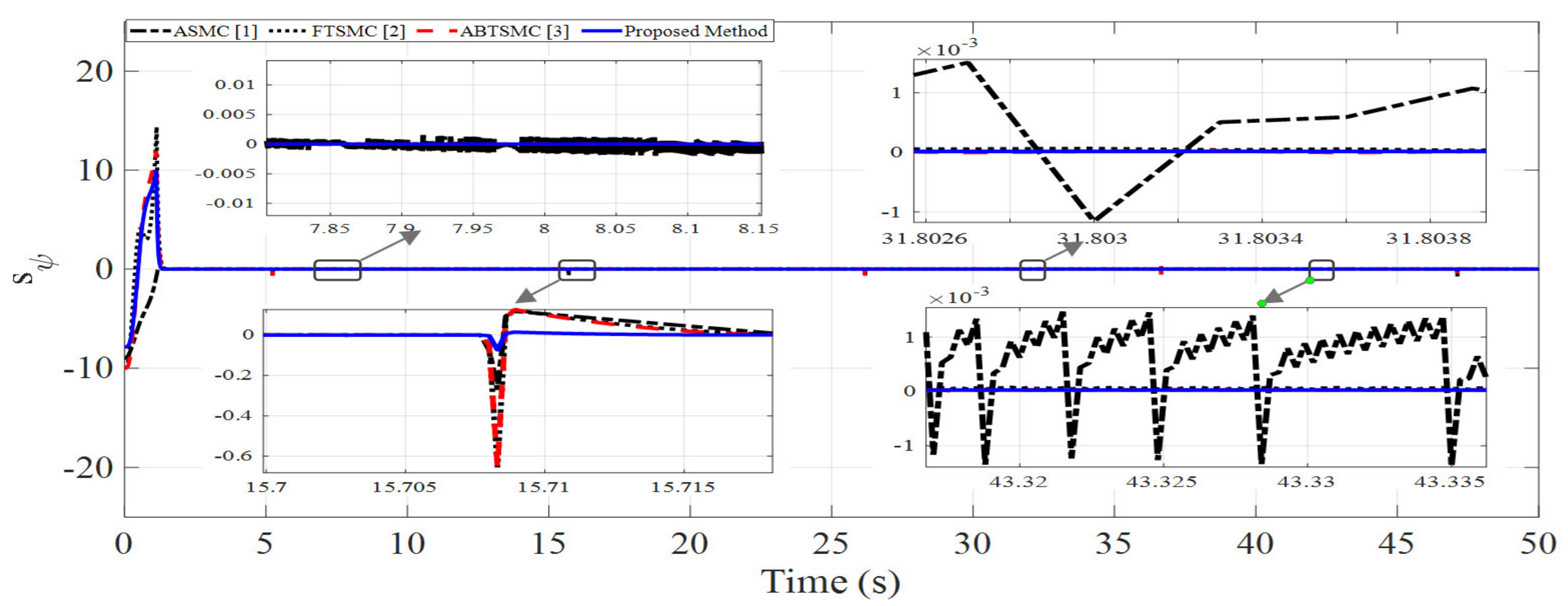
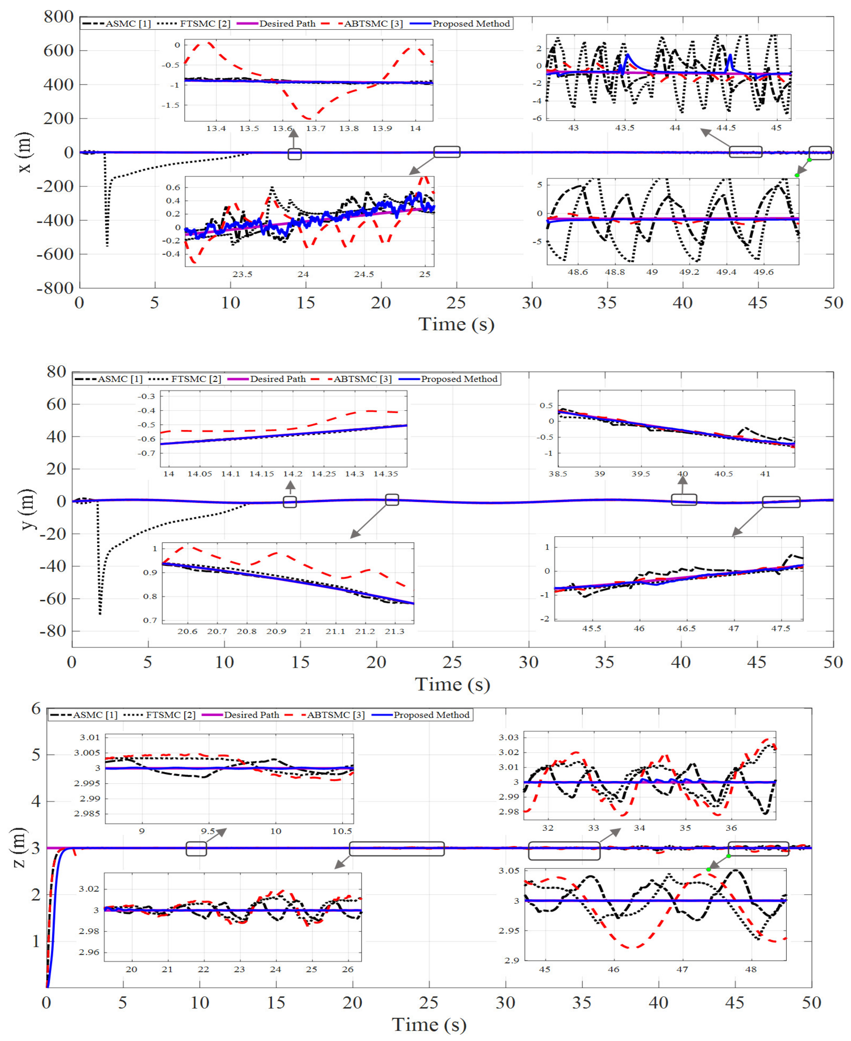
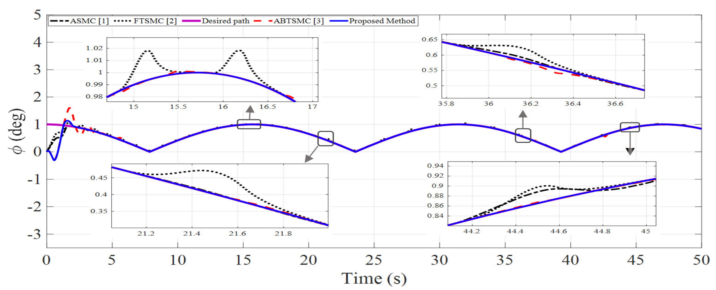
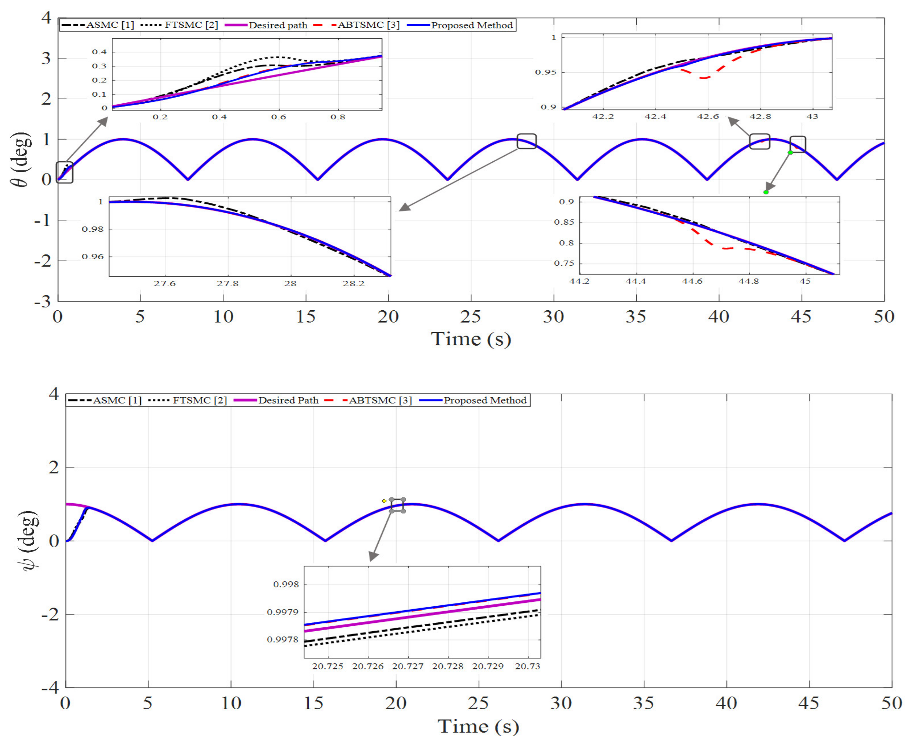
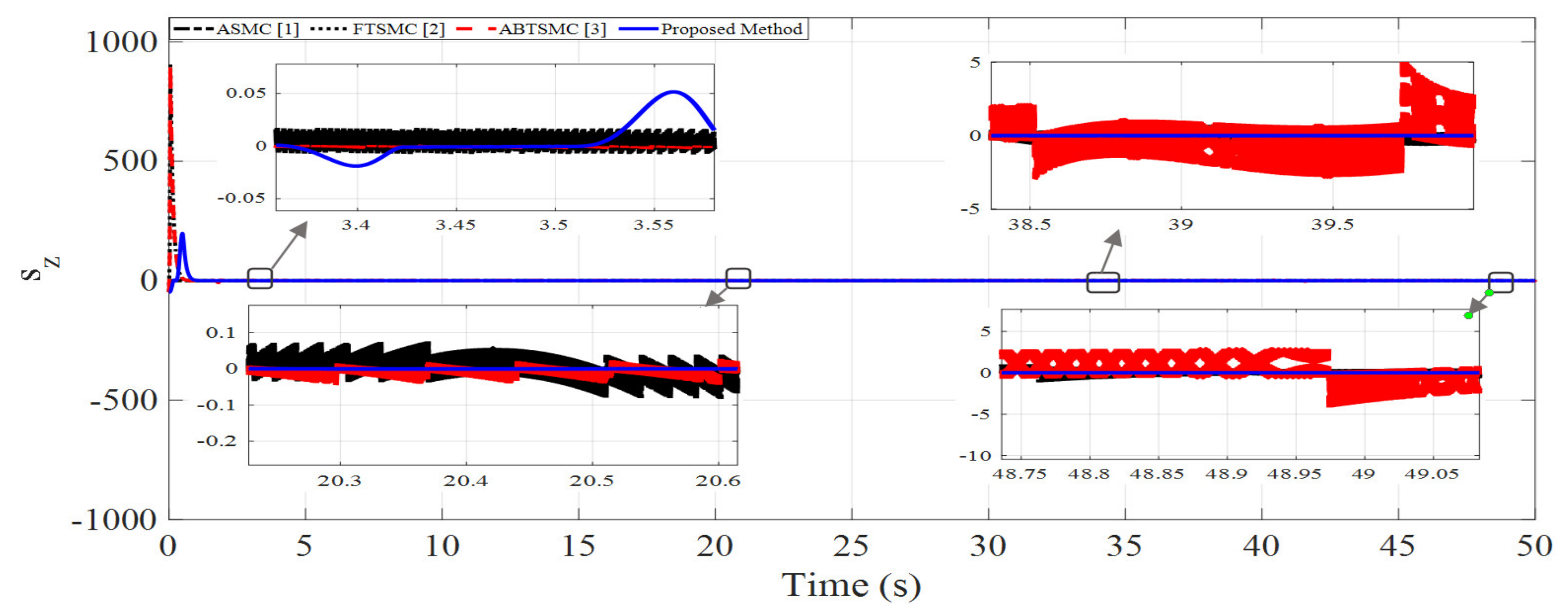
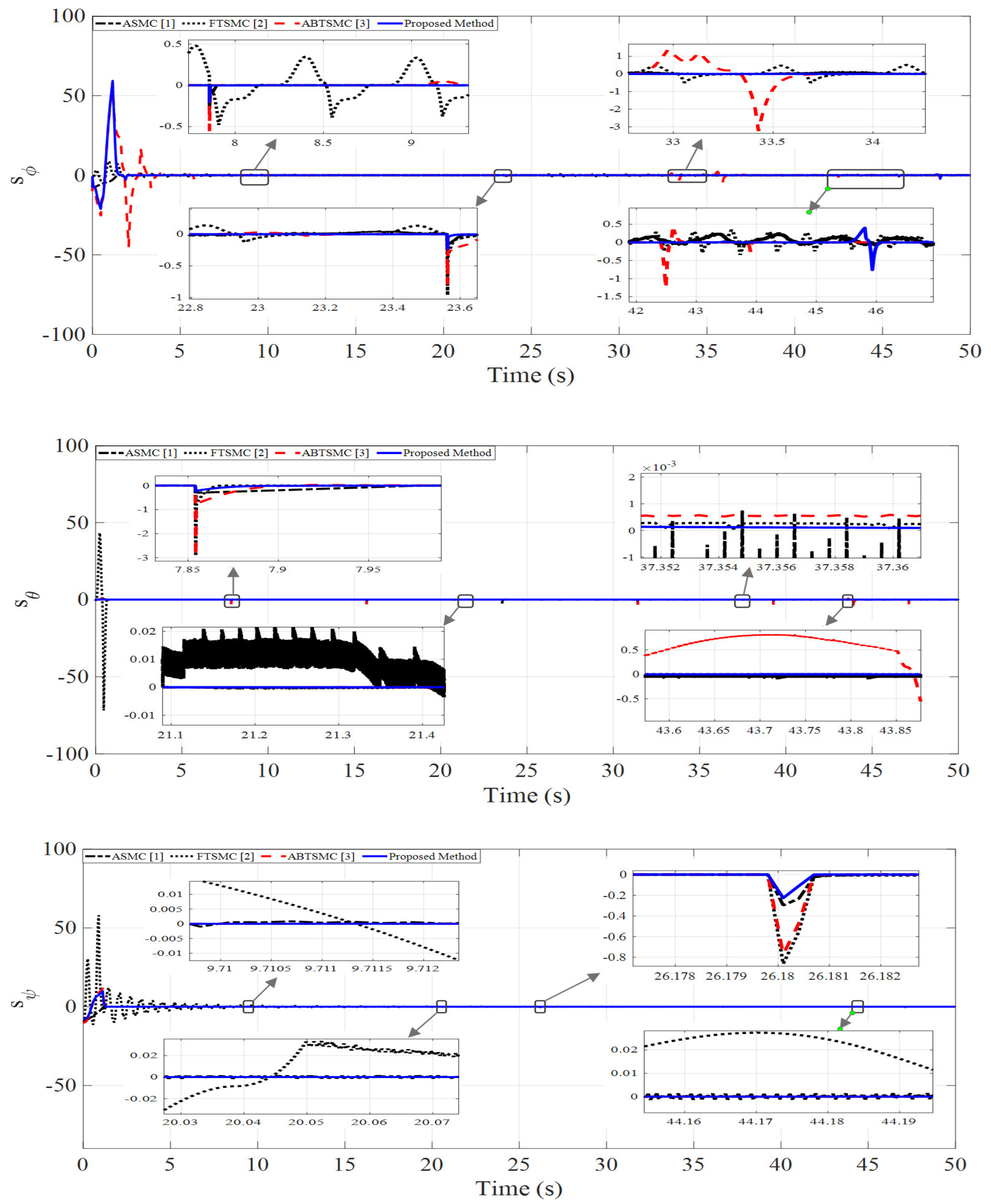
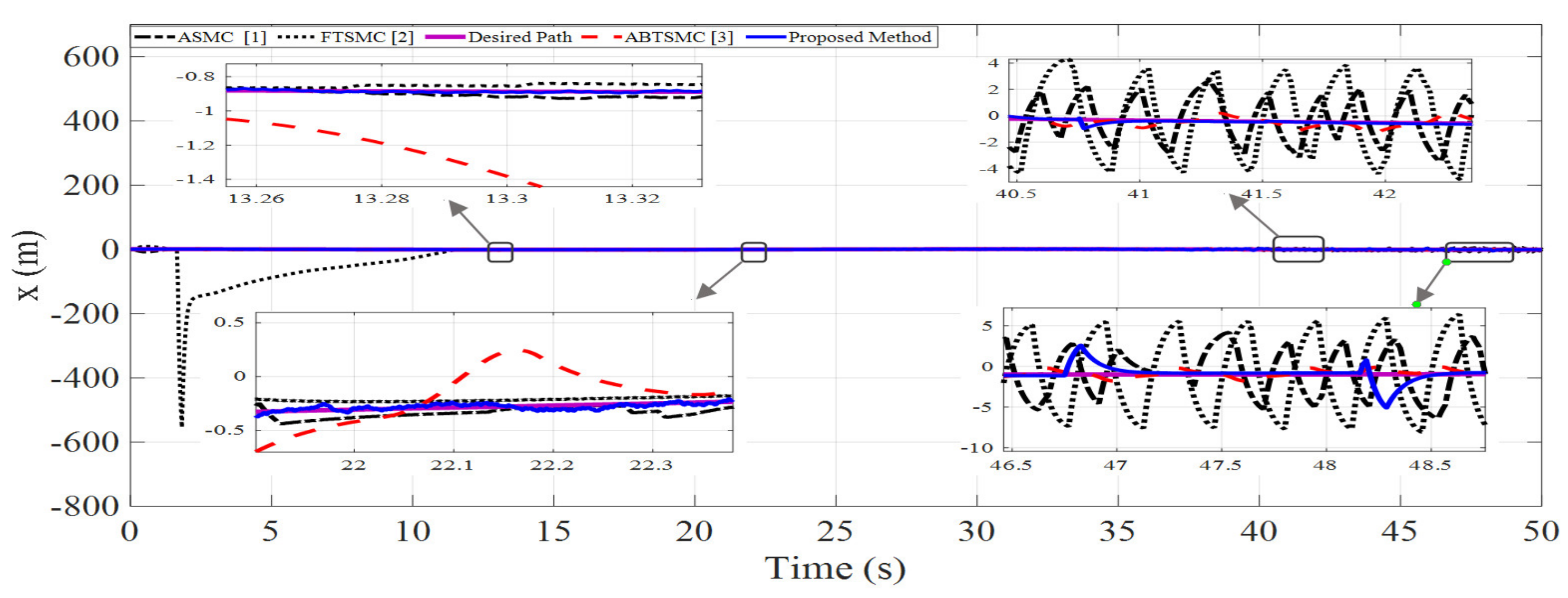
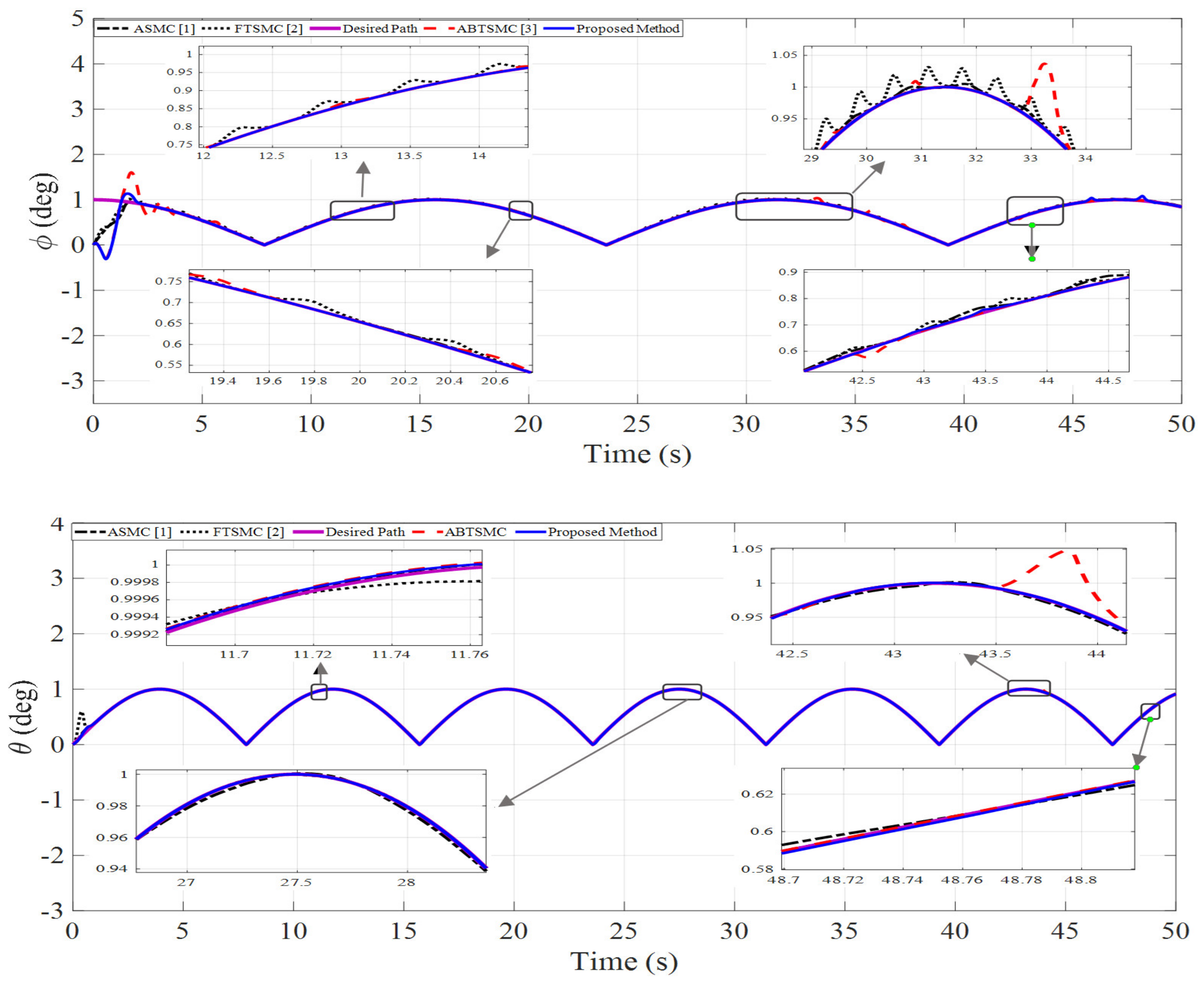
4. Simulation Results

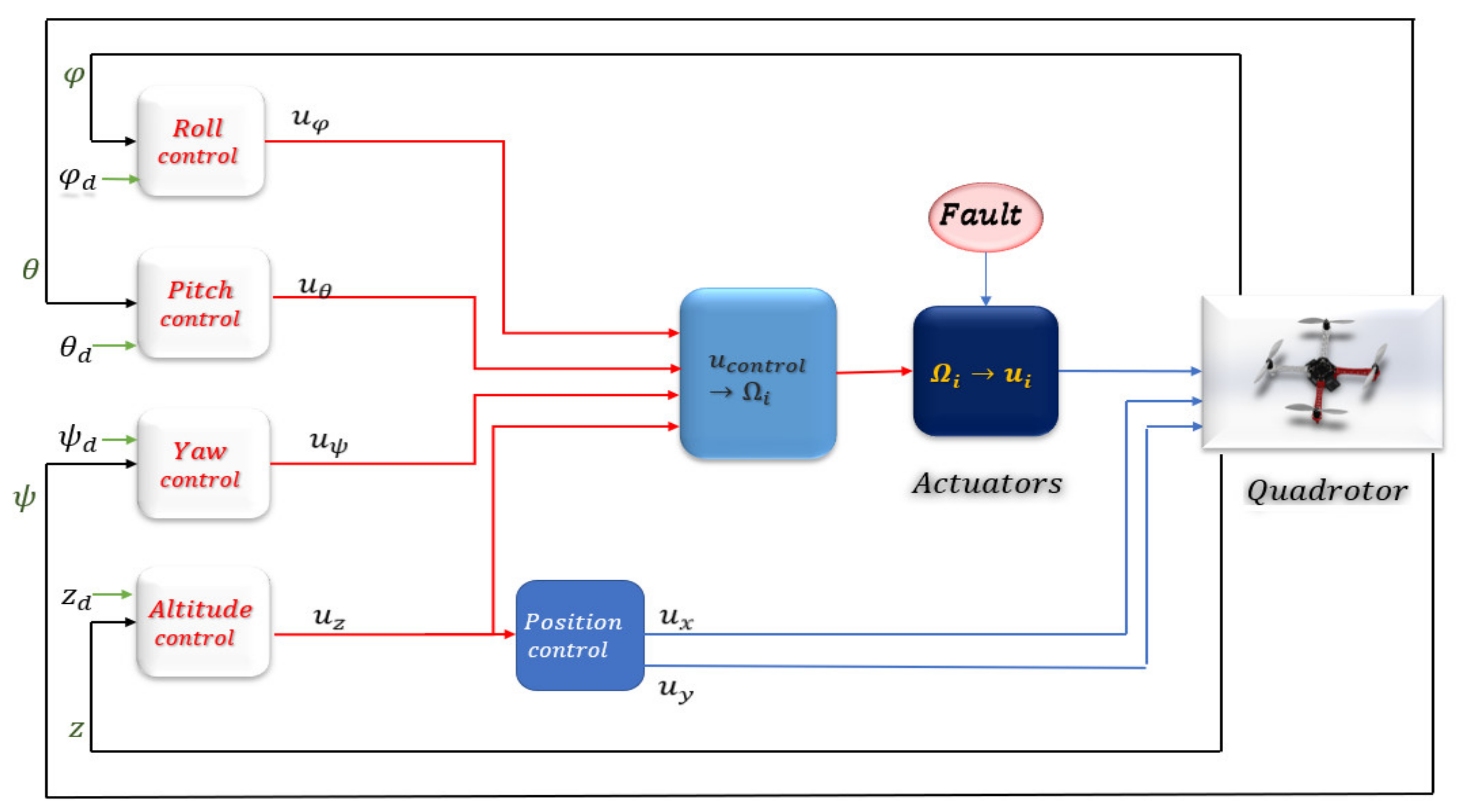
Before starting the scenarios and showing the simulation results, the general schematic of the system and the location of the fault and disturbance terms as well as the way that the controller works in the quadrotor system should be described. It should be stated that the quadrotor consists of several parts:

• Input controller;
• Quadrotor actuators;
• General quadrotor system;
• System output.

In the part of the actuators, as shown in Figure 1, the actuator fault reduced the effectiveness of the rotors and the output from the actuators was entered into the quadrotor system as the input of the system, and as a result, the output of the system was obtained. It should be noted that the perturbation was applied to the output part of the system according to Equation (1). By comparing the system output and the desired path and getting its error, the error signal was entered as the input of the sliding surface to the controller. With the help of the proposed control method (ABFTSMC), the resulting error was reduced and the effects of actuator fault, output disturbance, and parameter uncertainties were eliminated.

The performance of the adaptive barrier fast terminal sliding mode control (ABFTSMC) is assessed in this section. For performance analysis, in addition to the perturbations that enter the system, two types of actuator faults were considered. For comparison purposes, the performance of the proposed approach is compared with three methods: The first method is an adaptive sliding mode controller in [1] and the second method is the fast terminal sliding mode controller in [2]. Additionally, we performed a comparative analysis with the ABTSMC in [3]. The parameters of the quadrotor in this study are illustrated in

Table A1. Quadrotor parameters [54].

Parameter	Value	Unit	Parameter	Value	Unit
$g$	9.81	$\frac{\mathrm{m}}{{\mathrm{s}}^2}$	$J_r$	$90\times {10}^{-6}$	$\mathrm{kg}·{10}^{-6}$
$m$	1	$\mathrm{kg}$	$l$	0.24	$\mathrm{m}$
$I_x$	$8.1\times {10}^{-3}$	$\mathrm{kg}·{\mathrm{m}}^2$	$b$	$54\times {10}^{-6}$	$\mathrm{N}·{\mathrm{m}}^2$
$I_y$	$8.1\times {10}^{-3}$	$\mathrm{kg}·{\mathrm{m}}^2$	$d$	$1.1\times {10}^{-6}$	$\mathrm{N}·\mathrm{m}·{\mathrm{s}}^2$
$I_z$	$14\times {10}^{-3}$	$\mathrm{kg}·{\mathrm{m}}^2$

. The controller parameters are also given in

Table 1. Desired path and disturbances.

Variable	Value	Variable	Value
$b_1$ = $b_2$ for ($u_z$)	5	$b_1$ = $b_2$ for ($u_{\phi }$,$u_{\theta },u_{\psi }$)	9
$\alpha$	2	$Q_{psb}$	0
$\beta$	3	$\mu$	5
$\rho$	5	$\zeta$	1

. The results are illustrated by using the following scenarios:

Scenario 1: In the first scenario, the performance comparison was conducted with a 40% loss of control effectiveness by multiplicative sinusoidal fault in actuators 2 and 3. The faults were injected at the 20th second. One of the reasons for this type of fault is cracking or breakage of the rotor blades. In this scenario, 40% of the multiplicative sinus fault was applied to actuators 2 and 3. The desired trajectories and the amount of output perturbation are given in

Table 2. Desired path and disturbances.

State	Desired Path	Disturbance
$x_d$	$\left|\mathit{cos}(0.2t)\right|$	$10\mathit{sin}(0.0015t)$
$y_d$	$\left|\mathit{sin}(0.4t)\right|$	$5\mathit{sin}(0.0015t)$
$z_d$	3	$10\mathit{sin}(0.0015t)$
${\phi }_d$	$\left|\mathit{cos}(0.2t)\right|$	$10\mathit{sin}(0.0015t)$
${\theta }_d$	$\left|\mathit{sin}(0.4t)\right|$	$10\mathit{sin}(0.015t)$
${\psi }_d$	$\left|\mathit{cos}(0.3t)\right|$	$10\mathit{sin}(0.0015t)$

. The simulation results are illustrated in Figure 1, Figure 2 and Figure 3 via the comparison of methods [1,2,3] and the proposed ABFTSMC technique based on the tanh(.) function.

Figure 2 shows a comparison between the sliding surfaces of all three methods. In the case of variable z, methods [1,2,3] had high chattering. The proposed ABFTSMC method based on the tanh(.) function drastically reduced this value and damage to the system. This method worked similarly in other cases ($\phi ,\theta ,\psi$) and converged the sliding surface to zero with more minor error. Figure 3 and Figure 4 display the performance tracking of the quadrotor attitude and position.

Figure 3 shows the performance tracking of the quadrotor position $\left(x,y,z\right)$. As can be seen, the proposed controller, which is an adaptive barrier fast terminal sliding mode control and modified by a hyperbolic tangent, significantly reduced output chattering. The perturbation and fault of the actuator imposed so much instability on the system that the proposed method had better performance compared to methods [1,2,3] and followed the defined path with a slight error, where Figure 3 shows that the initial time reached the desired path in the finite time. The desired path tracked faster and with the least chattering and error. Figure 4 shows the $\left(x,y,z\right)$ performance tracking of the quadrotor attitude. As is known, the proposed controller had a more successful performance than the methods. The proposed method sped up the system response, converged to the desired trajectories, and tracked the trajectory with minimal error and chattering. Three examples of performance indicators, such as the integral of the absolute value of error (IAE), integral of the squared error (ISE), and integral of the time-weighted absolute error (ITAE), are examined in

Table 3. Performance indices under 40% sinusoidal fault actuators 2 and 3.

	States	$\mathit{x}$	$\mathit{y}$	$\mathit{z}$	$\mathit{\phi }$	$\mathit{\theta }$	$\mathit{\psi }$
	ASMC [1]	$90.17$	$915$	$1.188$.	$1.236$	$0.002245$	$0.5868$
ISE	FTSMC [2]	$11,040$	$390.15$	$3.254$	$0.5127$	$0.004933$	$0.5559$
ISE	ABTSMC [3]	$13.35$	$0.2575$	$1.211$	$1.414$	$0.001146$	$0.6035$
	Proposed method	$11.6$	$0.01381$	$1.173$	$0.3965$	$0.00081$	$0.4428$
	ASMC [1]	$27.35$	$3.129$	$1.162$	$1.268$	$0.07129$	$0.7905$
	FTSMC [2]	$828.4$	$62.1$	$1.496$	$1.133$	$0.05958$	$0.774$
IAE	ABTSMC [3]	$19.268$	$3.1$	$1.405$	$1.847$	$0.0506$	$0.776$
	Proposed method	$11.27$	$0.2956$	$1.055$	$0.89$	$0.03881$	$0.7498$
	ASMC [1]	$868$	$76.37$	$17.76$	$3.761$	$1.369$	$0.4188$
	FTSMC [2]	$5312$	$81.76$	$13.79$	$9.218$	$0.5146$	$0.3896$
ITAE	ABTSMC [3]	$479.3$	$73.26$	$25.51$	$5.113$	$0.9975$	$0.3771$
	Proposed method	$433.6$	$12.56$	$0.37818$	$1.096$	$0.2571$	$0.3672$

, which confirms the simulation results of Figure 3 and Figure 4 and the proper performance of the proposed method compared to the other methods. In all three comparative cases, the values of IAE, ISE, and ITAE in all six output modes in the proposed method were lower than with the other approaches.

Scenario 2: In this scenario, a loss of 50% control effectiveness by a multiplicative step fault in actuators 1 and 2 was imposed. These faults were injected at the 20th second. In this scenario, actuators 1 and 2 received a 50% step fault. The desired path is given in Table 2. In each scenario, the value of $\overline{t}$ in Equation (21) for each subsystem is written as follows:

$${\overline{t}}_{{\left[u_z,u_{\phi },u_{\theta },u_{\psi }\right]}^T}=\left[\begin{array}{c}0.865\\ 2.1\\ 1.4\\ 1.38\end{array}\right]$$

The simulation results are similar to the results of the first scenario, where the results of control methods [1,2,3] are compared with those of the proposed ABFTSMC method based on the hyperbolic tangent function, and are shown in Figure 5, Figure 6 and Figure 7, respectively. In all four sliding surfaces that correspond to the $\left(z,\phi ,\theta ,\psi \right)$ modes, it is clear that the sliding surface of the proposed method had the least chattering. In case z, papers [1,2,3] had high chattering, which caused serious damage, but the proposed method greatly reduced the chattering phenomenon.

The ABTSMC method [3] had higher chattering in the sliding surfaces compared to the other two methods. However, the proposed method reduced the chattering to approximately zero with the least error. According to Figure 6 and Figure 7, it is clear that all six system outputs experienced a lot of instability and chattering by applying the actuator fault after the 20th second. All three methods were able to solve this problem to some extent. However, the method mentioned in this paper, firstly, due to the barrier function, was able to limit the chattering due to output disturbances, parametric uncertainties, and actuator faults. Secondly, the main advantage of this method is the use of the continuous hyperbolic tangent function instead of the discontinuous sign function, which was able to reduce the chattering caused by the sign function and other disorders compared to other methods.

Table 4. Performance indices under 50% step fault in actuators 1 and 2.

	States	$\mathit{x}$	$\mathit{y}$	$\mathit{z}$	$\mathit{\phi }$	$\mathit{\theta }$	$\mathit{\psi }$
	ASMC [1]	$95.92$	$1.791$	$1.187$	$1.419$	$0.0008$	$0.6196$
ISE	FTSMC [2]	$11,045$	$3960$	$1.162$	$0.5541$	$0.04088$	$0.6026$
ISE	ABTSMC [3]	$15.52$	$0.2473$	$1.207$	$1.239$	$0.00229$	$0.6031$
	Proposed method	$11.51$	$0.01593$	$0.4741$	$0.4741$	$0.0007$	$0.442$
	ASMC [1]	$29.12$	$3.033$	$1.364$	$1.282$	$0.07129$	$0.8093$
	FTSMC [2]	$826.1$	$16.23$	$1.523$	$1.33$	$0.1405$	$1.078$
IAE	ABTSMC [3]	$19.26$	$2.932$	$1.162$	$1.926$	$0.08221$	$0.778$
	Proposed method	$11.48$	$0.3401$	$1.044$	$0.9746$	$0.04334$	$0.775$
	ASMC [1]	$951.6$	$8116$	$68.18$	$9.631$	$2.387$	$0.4136$
	FTSMC [2]	$5216$	$74.67$	$18.185$	$12.35$	$4.432$	$0.3764$
ITAE	ABTSMC [3]	$476$	$65.18$	$17.62$	$5.766$	$3.492$	$0.386$
	Proposed method	$442.4$	$14.49$	$13.46$	$3.969$	$0.7044$	$0.3448$

compares the indicator performance of the three methods applied to the quadrotor. This table shows that in all three indicators, IAE, ITAE, and ISE, the numbers obtained from the proposed method had the lowest value in all six output modes, indicating the superior performance of the proposed controller.

Remark 4.

It should be noted that scenarios 1 and 2 have the following differences:

-

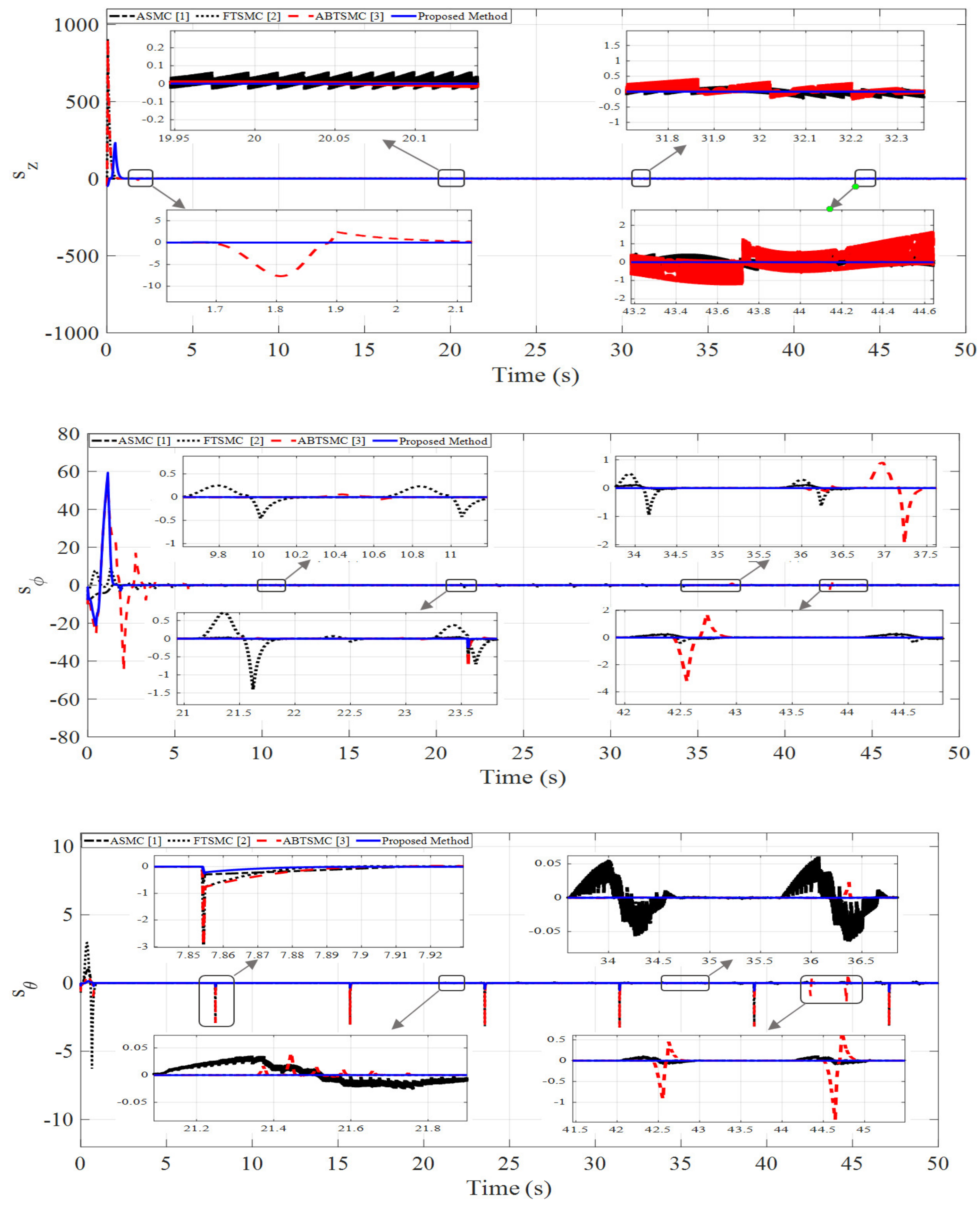
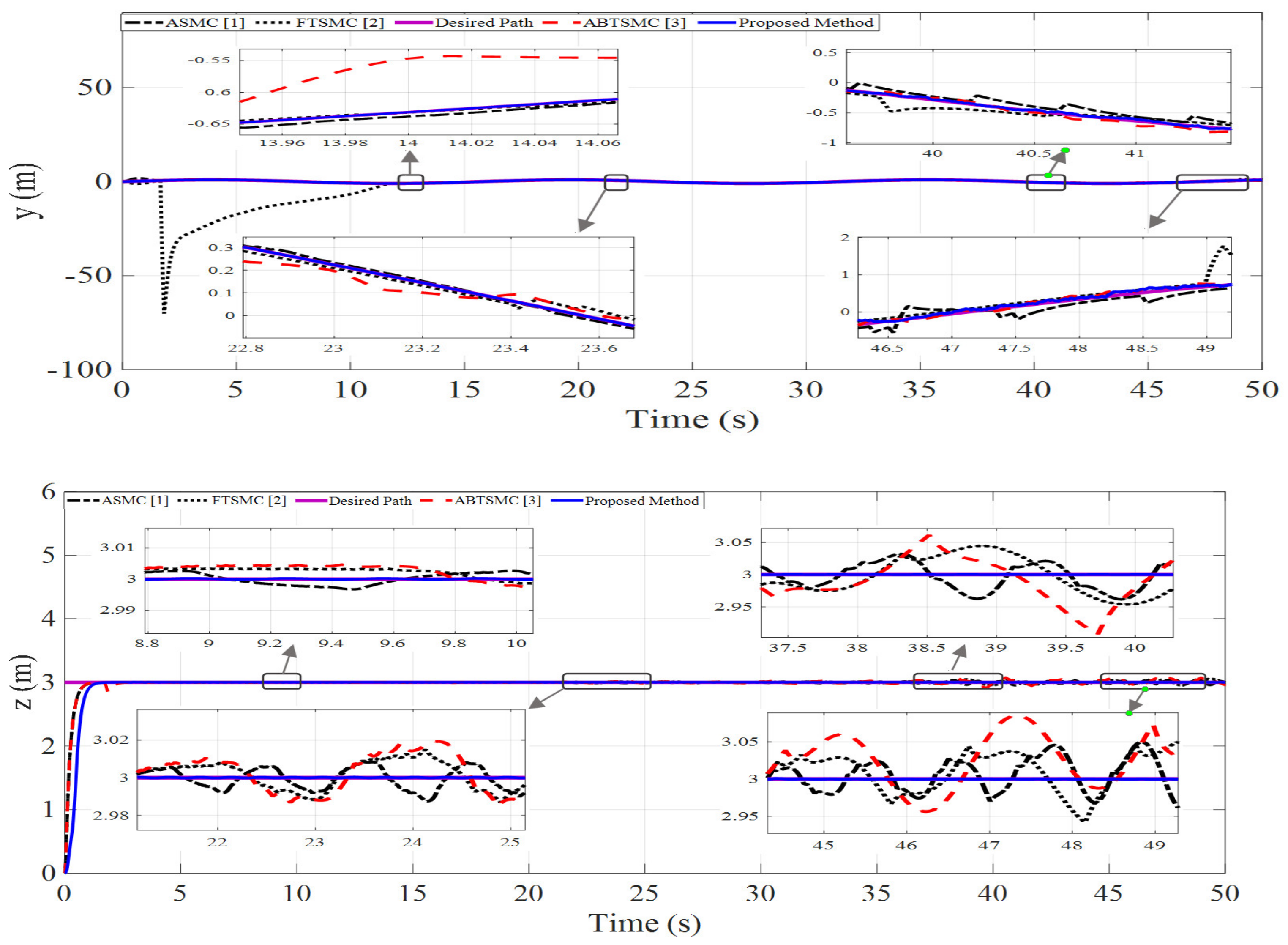
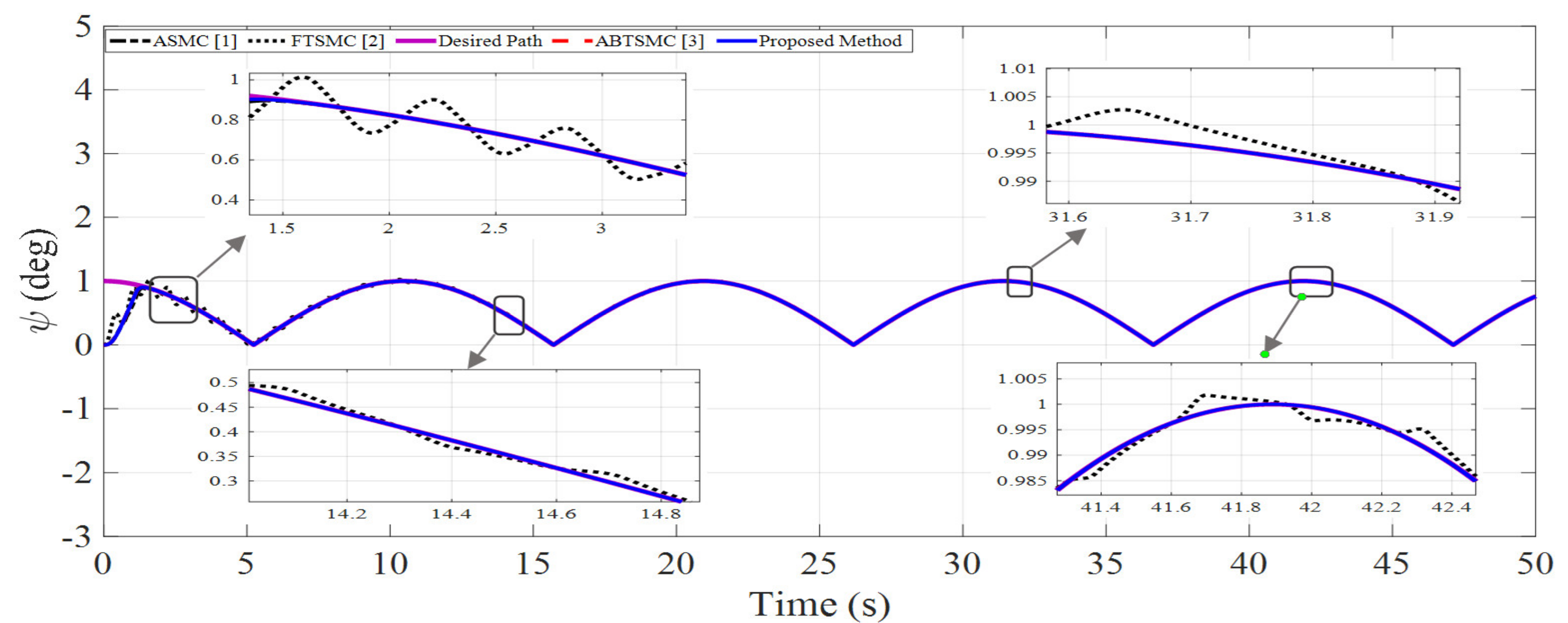
In the first scenario, 40% of the fault was entered into the system, but in scenario 2, the amount of this fault was 50% in the form of loss of rotor efficiency.

-

In the first scenario, the type of sinusoidal fault was intermittent, which sometimes results from cracking of the rotor blades, but the type of fault in the second scenario was a fixed-step function.

-

In the first scenario, fault was entered in actuators 2 and 3, but in the second scenario, it was applied to actuators 1 and 2.

5. Conclusions and Future Works

This paper proposed an adaptive barrier FTSMC based on the hyperbolic tangent function for quadrotor UAVs. The approach aims to eliminate the influences of external disturbances and mitigate the effects of the actuator faults and nonlinear uncertainties. This approach achieves three important objectives: (1) FTSMC provides the convergence performance in both reaching and sliding phases in the finite time, (2) an adaptive barrier function is used to ensure the convergence of the output variables independent of high gain of the disturbance and without overshoot, and (3) in order to reduce the severe chattering phenomenon, a hyperbolic tangent function is used instead of the sign function, which is effective in the simulation results. The simulation results and the performance index table show the effectiveness of this method in mitigating the actuator faults. A comparison analysis with the adaptive sliding mode control and fast terminal sliding mode control approaches proposed in [1,2,3] shows that the proposed method outperforms the other approaches. In future work, fuzzy-based model-predictive control with higher-order sliding surfaces will be employed for robust tracking control of quadrotor UAVs.

References

1. Yang, P.; Liu, Z.; Wang, Y.; Li, D. Adaptive sliding mode fault-tolerant control for uncertain systems with time delay. Int. J. Autom. Technol. 2020, 14, 337–345. [Google Scholar] [CrossRef]
2. Labbadi, M.; Cherkaoui, M. Robust adaptive nonsingular fast terminal sliding-mode tracking control for an uncertain quadrotor UAV subjected to disturbances. ISA Trans. 2020, 99, 290–304. [Google Scholar] [CrossRef] [PubMed]
3. Alattas, K.A.; Mofid, O.; Alanazi, A.K.; Abo-Dief, H.M.; Bartoszewicz, A.; Bakouri, M.; Mobayen, S. Barrier Function Adaptive Nonsingular Terminal Sliding Mode Control Approach for Quad-Rotor Unmanned Aerial Vehicles. Sensors 2022, 22, 909. [Google Scholar] [CrossRef]
4. Yang, P.; Wang, Z.; Zhang, Z.; Hu, X. Sliding Mode Fault Tolerant Control for a Quadrotor with Varying Load and Actuator Fault. Actuators 2021, 10, 323. [Google Scholar] [CrossRef]
5. Tang, P.; Lin, D.; Zheng, D.; Fan, S.; Ye, J. Observer based finite-time fault tolerant quadrotor attitude control with actuator faults. Aerosp. Sci. Technol. 2020, 104, 105968. [Google Scholar] [CrossRef]
6. Drozeski, G.R. A Fault-Tolerant Control Architecture for Unmanned Aerial Vehicles; Georgia Institute of Technology: Atlanta, GA, USA, 2005. [Google Scholar]
7. Alkadi, R.; Alnuaimi, N.; Yeun, C.; Shoufan, A. Blockchain Interoperability in Unmanned Aerial Vehicles Networks: State-of-the-art and Open Issues. IEEE Access 2022, 10, 14463–14479. [Google Scholar] [CrossRef]
8. Alattas, K.A.; Vu, M.T.; Mofid, O.; El-Sousy, F.F.; Fekih, A.; Mobayen, S. Barrier Function-Based Nonsingular Finite-Time Tracker for Quadrotor UAVs Subject to Uncertainties and Input Constraints. Mathematics 2022, 10, 1659. [Google Scholar] [CrossRef]
9. Mofid, O.; Mobayen, S.; Zhang, C.; Esakki, B. Desired tracking of delayed quadrotor UAV under model uncertainty and wind disturbance using adaptive super-twisting terminal sliding mode control. ISA Trans. 2022, 123, 455–471. [Google Scholar] [CrossRef]
10. Maddikunta, P.K.R.; Hakak, S.; Alazab, M.; Bhattacharya, S.; Gadekallu, T.R.; Khan, W.Z.; Pham, Q.-V. Unmanned aerial vehicles in smart agriculture: Applications, requirements, and challenges. IEEE Sens. J. 2021, 21, 17608–17619. [Google Scholar] [CrossRef]
11. Blanke, M.; Kinnaert, M.; Lunze, J.; Staroswiecki, M.; Schröder, J. Diagnosis and Fault-Tolerant Control; Springer: Berlin/Heidelberg, Germany, 2006; Volume 2. [Google Scholar]
12. Sadeghzadeh, I.; Zhang, Y. A review on fault-tolerant control for unmanned aerial vehicles (UAVs). Infotech@ Aerosp. 2011, 2011, 1472. [Google Scholar]
13. Najafi, A.; Bustan, D. Multiple actuator fault diagnosis based on parity space for quadrotor system. J. Aeronaut. Eng. 2020, 22, 1–11. [Google Scholar]
14. Fekih, A.; Mobayen, S.; Chen, C.-C. Adaptive Robust Fault-Tolerant Control Design for Wind Turbines Subject to Pitch Actuator Faults. Energies 2021, 14, 1791. [Google Scholar] [CrossRef]
15. Bustan, D.; Sani, S.H.; Pariz, N. Adaptive fault-tolerant spacecraft attitude control design with transient response control. IEEE/ASME Trans. Mechatron. 2013, 19, 1404–1411. [Google Scholar]
16. Zhang, Y.; Guan, Y.; Jiang, Y.; Chen, X. Lmi-based design of robust fault-tolerant controller. In Proceedings of the 2010 3rd International Symposium on Systems and Control in Aeronautics and Astronautics, Harbin, China, 8–10 June 2010; pp. 353–356. [Google Scholar]
17. Yang, G.-H.; Ye, D. Adaptive fault-tolerant H∞ control against sensor failures. IET Control Theory Appl. 2008, 2, 95–107. [Google Scholar] [CrossRef]
18. Wang, Y.; Jiang, B.; Wu, Z.-G.; Xie, S.; Peng, Y. Adaptive sliding mode fault-tolerant fuzzy tracking control with application to unmanned marine vehicles. IEEE Trans. Syst. Man Cybern. Syst. 2020, 51, 6691–6700. [Google Scholar] [CrossRef]
19. Zhao, Y.; Wang, J.; Yan, F.; Shen, Y. Adaptive sliding mode fault-tolerant control for type-2 fuzzy systems with distributed delays. Inf. Sci. 2019, 473, 227–238. [Google Scholar] [CrossRef]
20. Qinglei, H.; Zhang, Y.; Xing, H.; Bing, X. Adaptive integral-type sliding mode control for spacecraft attitude maneuvering under actuator stuck failures. Chin. J. Aeronaut. 2011, 24, 32–45. [Google Scholar]
21. Xu, S.S.-D.; Chen, C.-C.; Wu, Z.-L. Study of nonsingular fast terminal sliding-mode fault-tolerant control. IEEE Trans. Ind. Electron. 2015, 62, 3906–3913. [Google Scholar] [CrossRef]
22. Li, Y.; Sun, K.; Tong, S. Observer-based adaptive fuzzy fault-tolerant optimal control for SISO nonlinear systems. IEEE Trans. Cybern. 2018, 49, 649–661. [Google Scholar] [CrossRef]
23. Zou, A.-M.; Kumar, K.D. Adaptive fuzzy fault-tolerant attitude control of spacecraft. Control Eng. Pract. 2011, 19, 10–21. [Google Scholar] [CrossRef]
24. Jin, X.; Zhao, X.; Yu, J.; Wu, X.; Chi, J. Adaptive fault-tolerant consensus for a class of leader-following systems using neural network learning strategy. Neural Netw. 2020, 121, 474–483. [Google Scholar] [CrossRef] [PubMed]
25. Li, X.-J.; Yang, G.-H. Neural-network-based adaptive decentralized fault-tolerant control for a class of interconnected nonlinear systems. IEEE Trans. Neural Netw. Learn. Syst. 2016, 29, 144–155. [Google Scholar] [CrossRef] [PubMed]
26. Maciejowski, J.M.; Jones, C.N. MPC fault-tolerant flight control case study: Flight 1862. IFAC Proc. Vol. 2003, 36, 119–124. [Google Scholar] [CrossRef] [Green Version]
27. Sun, S.; Dong, L.; Li, L.; Gu, S. Fault-tolerant control for constrained linear systems based on MPC and FDI. Int. J. Inf. Syst. Sci. 2008, 4, 512–523. [Google Scholar]
28. Barghandan, S.; Badamchizadeh, M.A.; Jahed-Motlagh, M.R. Improved adaptive fuzzy sliding mode controller for robust fault tolerant of a quadrotor. Int. J. Control Autom. Syst. 2017, 15, 427–441. [Google Scholar] [CrossRef]
29. Chen, F.; Zhang, K.; Wang, Z.; Tao, G.; Jiang, B. Trajectory tracking of a quadrotor with unknown parameters and its fault-tolerant control via sliding mode fault observer. Proc. Inst. Mech. Eng. Part I J. Syst. Control. Eng. 2015, 229, 279–292. [Google Scholar] [CrossRef]
30. Mallavalli, S.; Fekih, A. Sliding mode-based fault tolerant control designs for quadrotor UAVs-A comparative study. In Proceedings of the 2017 13th IEEE International Conference on Control & Automation (ICCA), Ohrid, Macedonia, 3–6 July 2017; pp. 154–159. [Google Scholar]
31. Ullah, S.; Iqbal, K.; Malik, F.M. Fault-Tolerant Sliding Mode Control of a Quadrotor UAV with Delayed Feedback. Int. J. Mech. Eng. Robot. Res. 2020, 9, 1–6. [Google Scholar] [CrossRef]
32. Wang, Z.; Yang, P.; Hu, X.; Zhang, Z.; Wen, C. Sliding Mode Fault Tolerant Control of Quadrotor Uav with State Constraints Under Actuator Fault. Int. J. Innov. Comput. Inf. Control. 2021, 17, 639–653. [Google Scholar]
33. Aguilar-Ibanez, C.; Moreno-Valenzuela, J.; García-Alarcón, O.; Martinez-Lopez, M.; Acosta, J.Á.; Suarez-Castanon, M.S. PI-type controllers and Σ–Δ modulation for saturated DC-DC buck power converters. IEEE Access 2021, 9, 20346–20357. [Google Scholar] [CrossRef]
34. Balcazar, R.; Rubio, J.d.J.; Orozco, E.; Andres Cordova, D.; Ochoa, G.; Garcia, E.; Pacheco, J.; Gutierrez, G.J.; Mujica-Vargas, D.; Aguilar-Ibañez, C. The Regulation of an Electric Oven and an Inverted Pendulum. Symmetry 2022, 14, 759. [Google Scholar] [CrossRef]
35. Rubio, J.D.J.; Orozco, E.; Cordova, D.A.; Islas, M.A.; Pacheco, J.; Gutierrez, G.J.; Zacarias, A.; Soriano, L.A.; Meda-Campaña, J.A.; Mujica-Vargas, D. Modified linear technique for the controllability and observability of robotic arms. IEEE Access 2022, 10, 3366–3377. [Google Scholar] [CrossRef]
36. Silva-Ortigoza, R.; Hernández-Márquez, E.; Roldán-Caballero, A.; Tavera-Mosqueda, S.; Marciano-Melchor, M.; Garcia-Sanchez, J.R.; Hernández-Guzmán, V.M.; Silva-Ortigoza, G. Sensorless Tracking Control for a “Full-Bridge Buck Inverter–DC Motor” System: Passivity and Flatness-Based Design. IEEE Access 2021, 9, 132191–132204. [Google Scholar] [CrossRef]
37. Soriano, L.A.; Rubio, J.d.J.; Orozco, E.; Cordova, D.A.; Ochoa, G.; Balcazar, R.; Cruz, D.R.; Meda-Campaña, J.A.; Zacarias, A.; Gutierrez, G.J. Optimization of sliding mode control to save energy in a SCARA robot. Mathematics 2021, 9, 3160. [Google Scholar] [CrossRef]
38. Soriano, L.A.; Zamora, E.; Vazquez-Nicolas, J.; Hernández, G.; Barraza Madrigal, J.A.; Balderas, D. PD control compensation based on a cascade neural network applied to a robot manipulator. Front. NeuroRobot. 2020, 14, 577749. [Google Scholar] [CrossRef]
39. Samir, B. Design and Control of Quadrotors with Application to Autonomous Flying. Ph.D. Thesis, Swiss Federal Institute of Technology, Lausanne, Switzerland, 2007. [Google Scholar]
40. Eliker, K.; Grouni, S.; Tadjine, M.; Zhang, W. Practical finite time adaptive robust flight control system for quad-copter UAVs. Aerosp. Sci. Technol. 2020, 98, 105708. [Google Scholar] [CrossRef]
41. Eliker, K.; Grouni, S.; Tadjine, M.; Zhang, W. Quadcopter nonsingular finite-time adaptive robust saturated command-filtered control system under the presence of uncertainties and input saturation. Nonlinear Dyn. 2021, 104, 1363–1387. [Google Scholar] [CrossRef]
42. Ejaz, F.; Hamayun, M.T.; Hussain, S.; Ijaz, S.; Yang, S.; Shehzad, N.; Rashid, A. An adaptive sliding mode actuator fault tolerant control scheme for octorotor system. Int. J. Adv. Robot. Syst. 2019, 16, 1729881419832435. [Google Scholar] [CrossRef] [Green Version]
43. Mallavalli, S.; Fekih, A. A fault tolerant tracking control for a quadrotor UAV subject to simultaneous actuator faults and exogenous disturbances. Int. J. Control 2020, 93, 655–668. [Google Scholar] [CrossRef]
44. Saggai, A.; Zeghlache, S.; Benyettou, L.; Djerioui, A. Fault Tolerant Control against Actuator Faults Based on Interval Type-2 Fuzzy Sliding Mode Controller for a Quadrotor Aircraft. In Proceedings of the 2020 2nd International Workshop on Human-Centric Smart Environments for Health and Well-being (IHSH), Boumerdes, Algeria, 9–10 February 2021; pp. 181–186. [Google Scholar]
45. Zeghlache, S.; Djerioui, A.; Benyettou, L.; Benslimane, T.; Mekki, H.; Bouguerra, A. Fault tolerant control for modified quadrotor via adaptive type-2 fuzzy backstepping subject to actuator faults. ISA Trans. 2019, 95, 330–345. [Google Scholar] [CrossRef]
46. Naseri, K.; Vu, M.T.; Mobayen, S.; Najafi, A.; Fekih, A. Design of Linear Matrix Inequality-Based Adaptive Barrier Global Sliding Mode Fault Tolerant Control for Uncertain Systems with Faulty Actuators. Mathematics 2022, 10, 2159. [Google Scholar] [CrossRef]
47. Nekoukar, V.; Dehkordi, N.M. Robust path tracking of a quadrotor using adaptive fuzzy terminal sliding mode control. Control Eng. Pract. 2021, 110, 104763. [Google Scholar] [CrossRef]
48. Wang, B.; Zhang, Y. An adaptive fault-tolerant sliding mode control allocation scheme for multirotor helicopter subject to simultaneous actuator faults. IEEE Trans. Ind. Electron. 2017, 65, 4227–4236. [Google Scholar] [CrossRef] [Green Version]
49. Izadi, H.A.; Zhang, Y.; Gordon, B.W. Fault tolerant model predictive control of quad-rotor helicopters with actuator fault estimation. IFAC Proc. Vol. 2011, 44, 6343–6348. [Google Scholar] [CrossRef] [Green Version]
50. Li, T.; Zhang, Y.; Gordon, B.W. Nonlinear fault-tolerant control of a quadrotor UAV based on sliding mode control technique. IFAC Proc. Vol. 2012, 45, 1317–1322. [Google Scholar] [CrossRef]
51. Wang, F.; Ma, Z.; Gao, H.; Zhou, C.; Hua, C. Disturbance Observer-based Nonsingular Fast Terminal Sliding Mode Fault Tolerant Control of a Quadrotor UAV with External Disturbances and Actuator Faults. Int. J. Control Autom. Syst. 2022, 20, 1122–1130. [Google Scholar] [CrossRef]
52. Wang, X.; van Kampen, E.-J.; Chu, Q. Quadrotor fault-tolerant incremental nonsingular terminal sliding mode control. Aerosp. Sci. Technol. 2019, 95, 105514. [Google Scholar] [CrossRef]
53. Li, X.; Zhang, H.; Fan, W.; Wang, C.; Ma, P. Finite-time control for quadrotor based on composite barrier Lyapunov function with system state constraints and actuator faults. Aerosp. Sci. Technol. 2021, 119, 107063. [Google Scholar] [CrossRef]
54. Wang, J.; Zhao, Z.; Zheng, Y. NFTSM-based Fault Tolerant Control for Quadrotor Unmanned Aerial Vehicle with Finite-Time Convergence. IFAC-PapersOnLine 2018, 51, 441–446. [Google Scholar] [CrossRef]
55. Li, T.; Zhang, Y.; Gordon, B.W. Passive and active nonlinear fault-tolerant control of a quadrotor unmanned aerial vehicle based on the sliding mode control technique. Proc. Inst. Mech. Eng. Part I J. Syst. Control Eng. 2013, 227, 12–23. [Google Scholar] [CrossRef]
56. Aghababa, M.P.; Akbari, M.E. A chattering-free robust adaptive sliding mode controller for synchronization of two different chaotic systems with unknown uncertainties and external disturbances. Appl. Math. Comput. 2012, 218, 5757–5768. [Google Scholar] [CrossRef]
57. Boukattaya, M.; Mezghani, N.; Damak, T. Adaptive nonsingular fast terminal sliding-mode control for the tracking problem of uncertain dynamical systems. ISA Trans. 2018, 77, 1–19. [Google Scholar] [CrossRef] [PubMed]
58. Labbadi, M.; Cherkaoui, M. Robust adaptive backstepping fast terminal sliding mode controller for uncertain quadrotor UAV. Aerosp. Sci. Technol. 2019, 93, 105306. [Google Scholar] [CrossRef]
59. Yu, X.; Zhihong, M. Fast terminal sliding-mode control design for nonlinear dynamical systems. IEEE Trans. Circuits Syst. I Fundam. Theory Appl. 2002, 49, 261–264. [Google Scholar]
60. Nguyen, V.-C.; Vo, A.-T.; Kang, H.-J. A finite-time fault-tolerant control using non-singular fast terminal sliding mode control and third-order sliding mode observer for robotic manipulators. IEEE Access 2021, 9, 31225–31235. [Google Scholar] [CrossRef]
61. Obeid, H.; Fridman, L.M.; Laghrouche, S.; Harmouche, M. Barrier function-based adaptive sliding mode control. Automatica 2018, 93, 540–544. [Google Scholar] [CrossRef]
62. Obeid, H.; Laghrouche, S.; Fridman, L.; Chitour, Y.; Harmouche, M. Barrier function-based adaptive super-twisting controller. IEEE Trans. Autom. Control 2020, 65, 4928–4933. [Google Scholar] [CrossRef] [Green Version]
63. Afshari, M.; Mobayen, S.; Hajmohammadi, R.; Baleanu, D. Global sliding mode control via linear matrix inequality approach for uncertain chaotic systems with input nonlinearities and multiple delays. J. Comput. Nonlinear Dyn. 2018, 13, 031008. [Google Scholar] [CrossRef]
64. Yau, H.-T. Design of adaptive sliding mode controller for chaos synchronization with uncertainties. Chaos Solitons Fractals 2004, 22, 341–347. [Google Scholar] [CrossRef]
Figure 1. The control scheme of the quadrotor.
Mathematics 10 03009 g001
Figure 2. Sliding surface under 40% sinusoidal fault to actuators 2 and 3.
Mathematics 10 03009 g002aMathematics 10 03009 g002b
Figure 3. Quadrotor position under 40% sinusoidal fault to actuators 2 and 3.
Mathematics 10 03009 g003
Figure 4. Quadrotor attitude under 40% sinusoidal fault in actuators 2 and 3.
Mathematics 10 03009 g004aMathematics 10 03009 g004b
Figure 5. Sliding surface under 50% step fault in actuators 1 and 2.
Mathematics 10 03009 g005aMathematics 10 03009 g005b
Figure 6. Quadrotor position under 50% step fault to actuators 1 and 2.
Mathematics 10 03009 g006aMathematics 10 03009 g006b
Figure 7. Quadrotor attitude under 50% step fault to actuator 1 and 2.
Mathematics 10 03009 g007aMathematics 10 03009 g007b