Two-State Alien Tiles: A Coding-Theoretical Perspective

Abstract

Most studies on the switching game Lights Out and its variants focus on the solvability of given games or the number of solvable games, but when the game is viewed in a coding-theoretical perspective, more interesting questions with special symbolizations in coding theory will naturally pop up, such as finding the minimal number of lit lights among all solvable games apart from the solved game, or finding the minimal number of lit lights that the player can achieve from a given unsolvable game, etc. However, these problems are usually hard to solve in general from the perspective of algorithmic complexity. This study considers a Lights Out variant called two-state Alien Tiles, which toggles all the lights in the same row and those in the same column of the clicked light. We investigate its properties, discuss several coding-theoretical problems about this game, and explore this game as an error-correcting code and investigate its optimality. The purpose of this paper is to propose ways of playing switching games in a think-outside-the-box manner, which benefits the recreational mathematics community.

1. Introduction

The mathematics of Lights Out was extensively studied in the past decades. The Lights Out game board is a rectangular grid of lights, where each light is either on (lit) or off (unlit). By performing a move, a selected light and its adjacent rectilinear neighbors are toggled. At the beginning of the game, some lights have already been switched on. The player is asked to solve the game, i.e., switching off all the lights, by performing a sequence of moves. Many variants such as the setting up of different toggle patterns were explored, e.g., in [1,2].

Regardless of the variant of Lights Out, most studies focused on the solvability (or the attainability) of given games or the number of solvable (or attainable) games. These problems can usually be solved efficiently by elementary linear algebra and group theory approaches, e.g., in [3,4]. More precisely, these problems are in the complexity class P. A brief introduction of algorithmic complexity can be found in the Supplementary Materials. In a nutshell, problems in P can be computed efficiently and are considered as simple mathematical problems. Sometimes, the analysis may require the use of other mathematical tools, such as Fibonacci polynomials [5] and cellular automata [6].

However, not every derived problem has a known algorithm for solving it in an efficient manner. For example, the shortest solution problem focuses on solving a game with minimal number of moves, which is related to the minimum distance decoding (or the maximum likelihood decoding) in coding theory. In a more general setting, this problem was proven to have no known efficient algorithms for solving [7,8]. Precisely, this problem is NP-hard and its decision problem is NP-complete. Approximating the solution within a constant factor is also NP-hard [9,10]. Yet, it is possible to solve the shortest solution problem efficiently if certain special properties of the game can be detected and found.

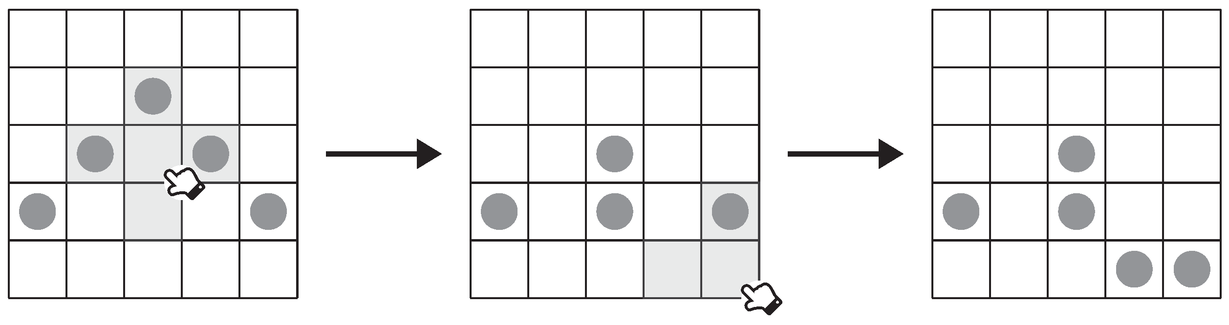
The motivation of this study is inspired by the Gale–Berlekamp switching game, a Lights Out variant such that the player can either toggle an entire row or an entire column per move. Example moves of a $5\times 5$ Gale–Berlekamp switching game are illustrated in Figure 1, where the gray cells indicate the toggle pattern. Despite the simple toggle patterns, Roth and Viswanathan [11] proved that finding the minimal number of lights that the player cannot switch off from a given Gale–Berlekamp switching game is NP-complete, although a linear time approximation algorithm was later discovered by Karpinski and Schudy [12].

This problem has a special symbolization in coding theory, and has attracted researchers to further investigate this game, e.g., [13,14,15]. In other words, when we view the game from a coding-theoretical perspective, we can ask more questions with special symbolizations in coding theory, such as:

• Hamming weight. What is the minimal number of lit lights among all solvable games except the solved game?
• Coset leader. Which game has the minimal number of lit lights that the player can achieve from a given game? What is this minimal number? How many such games can the player achieve?
• Covering radius. Among all possible games, what is the maximal number of lit lights that remained when the number of lit lights is minimized?
• Error correction. Which is the “closest” solvable game from a given unsolvable game in the sense of toggling the minimal number of individual lights? Furthermore, is such closest solvable game unique?

A brief introduction of coding theory can be found in the Supplementary Materials, which we discuss the physical meaning of the aforementioned terminologies in coding theory. Again, not all problems have known algorithms to be solved in an efficient manner. For example, the first problem about Hamming weight, which is also known as the minimum distance problem, is NP-hard in general [16].

Previous studies of switching games in recreational mathematics mostly focused on the solvability check, the way to solve a game, and the counting of the number of solvable games. On the other hand, the coding-theoretical view enhances the ways to play the games, but the existing studies mostly focused on the hardness results, e.g., for Gale–Berlekamp switching games and its generalization. One natural question to ask is as follows: Is there any commonly played switching game where its coding-theoretical results are not computationally hard? We give an affirmative answer to this question, which is the switching game that we are focusing within this study.

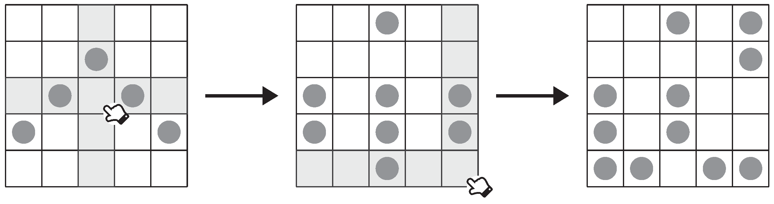
In this study, we consider a natural variant of Lights Out in a way that each toggle pattern is changed from a “small cross” to a “big cross” covering the entire row and the entire column. This variant is the two-state version of a game called Alien Tiles, where the original Alien Tiles has four states per light [17]. A comparison between the ordinary Lights Out and the two-state Alien Tiles is as illustrated in Figure 2 and Figure 3. The two-state Alien Tiles has a neat and simple parity condition, so that this game has various discussions on the Internet such as [18,19]. Similar setups also appear as training questions of programming contests [20]. The solvability and the number of solvable games of arbitrary-state Alien Tiles have been answered by Maier and Nickel [21]. However, the coding-theoretical problems that we listed above were not investigated, and we will answer these questions within this study.

This paper is organized as follows. We first discuss some general techniques for Lights Out and its two-state variants in Section 2. Next, we discuss the basic properties of two-state Alien Tiles in Section 3. We then solve our proposed coding-theoretical problems of the two-state Alien Tiles in Section 4. In Section 5, we apply the two-state Alien Tiles as an error-correcting code and investigate its optimality. Lastly, we discuss a states decomposition technique to link up the original four-state Alien Tiles and the two-state variant in Section 6, and then conclude this study in Section 7.

2. General Techniques for Lights out and Its Two-State Variants

We now describe some existing techniques in the literature for tackling Lights Out and its two-state variants.

2.1. Model

A general two-state Lights Out game consists of two basic elements:

• A game board of lights;
• A set of toggle patterns for toggling certain lights.

When we toggle the lights according to a toggle pattern, we say we apply (or perform) a move.

We first model the game board. For convenience, we use 1 to represent a lit light, and 0 to represent an unlit light. We consider an $m\times n$ grid of lights. Each possible grid can be represented by an $m\times n$ matrix over a binary field ${\mathbb{F}}_2$. A notable property of ${\mathbb{F}}_2$ is that the addition operation is having the same effect as the subtraction operation.

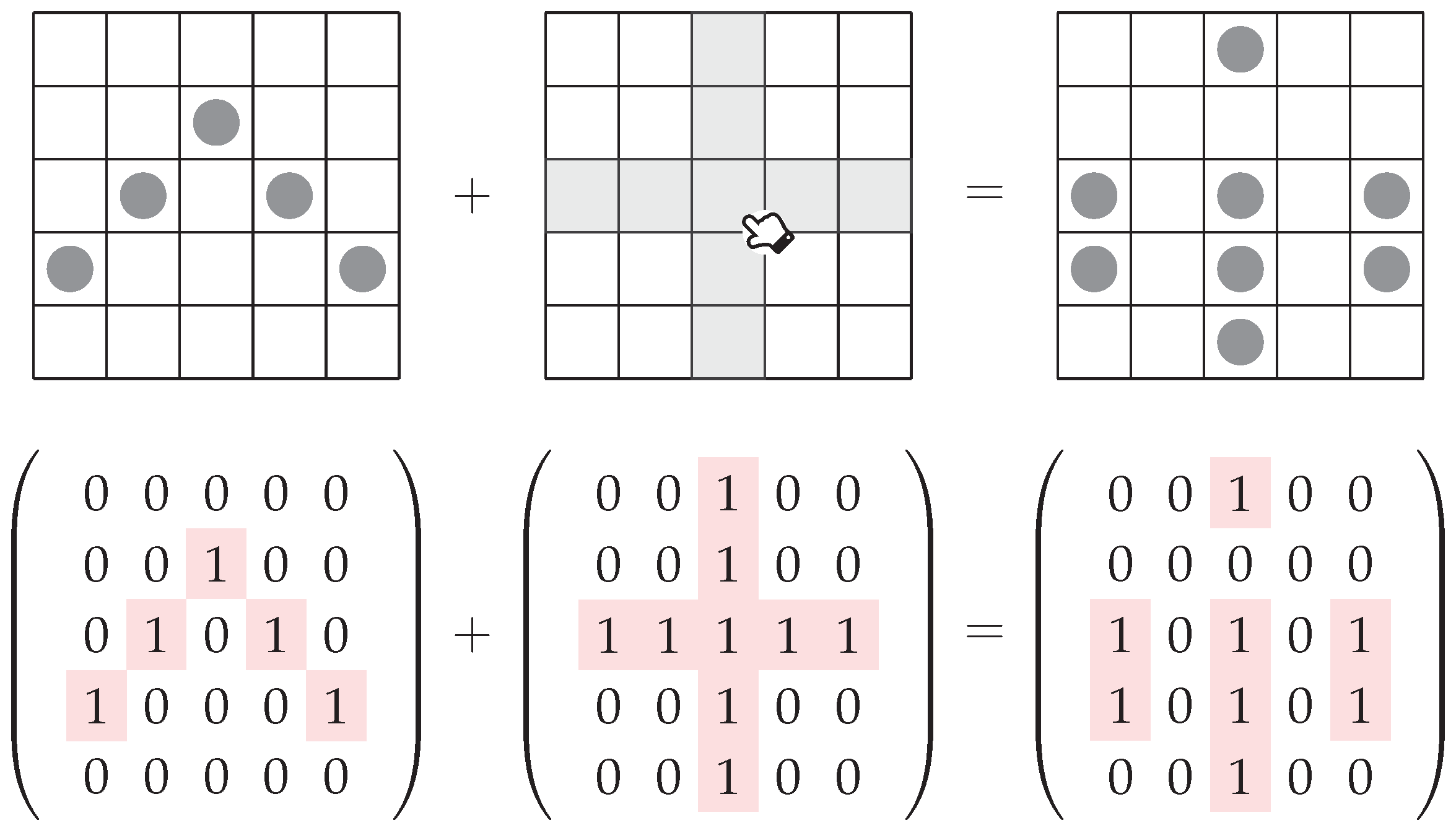
We can represent each toggle pattern by an $m\times n$ grid of lights, where each light in the grid is on if and only if the toggle pattern toggles this light. For example, the gray cells in Figure 2 and Figure 3 are the lit lights in the toggle pattern when the central light is clicked. Similarly, each toggle pattern is represented by an $m\times n$ matrix over ${\mathbb{F}}_2$. Throughout the process, we can model the game board after performing a move by matrix addition, i.e., the original game board matrix plus the toggle pattern matrix. Figure 4 illustrates an example of the model in matrix form.

To simplify the notations, we vectorize each $m\times n$ matrix into an $mn\times 1$ column vector by stacking the columns of the matrix on top of one another. The collection of all possible (vectorized) grids forms a vector space $G={\mathbb{F}}_2^{mn}$, which is called the game space. When it is clear from the context, we do not vectorize the matrix form of the game for readability. In a similar manner, we can transform an arbitrary-shape game board into a vector; thus, a similar vector space model also works for non-rectangular game boards.

Definition 1

(Solvability). A game $g\in G$ is solvable if and only if there exists a sequence of moves to switch g into a zero vector.The zero vector is also called a solved game.

The concept of solvability and attainability are similar. We mention both terminologies here because some literature, such as [21], consider attainability in lieu of solvability. A game $g\in G$ is attainable if and only if there exists a sequence of moves that can switch a zero vector into g.

We define the solvable game space by the vector space S over ${\mathbb{F}}_2$ spanned by the set of all vectorized toggle patterns. Note that $S\subseteq G$. A game g is solvable if and only if $g\in S$. This is due to the nature of the game that:

• Applying a move twice will not toggle any lights, i.e., apply the same move again will undo the move;
• Every permutation of a sequence of moves toggles the same set of lights, i.e., the order of the moves is not taken into consideration.

It is easy to observe that solvability is equivalent to attainability in Lights Out and its two-state variants: the sequence of moves that solves a game can also attain the game.

For most Lights Out variants, including the two-state Alien Tiles, we can model the moves in this manner. There are totally $mn$ toggle patterns, so there are $mn$ possible moves. We can bijectively associate each move by a light in the grid. For the two-state Alien Tiles, the $(i,j)$-th light in the grid is associated with the move that toggles all the lights in the i-th row and the j-th column. That is, this move is represented by a binary matrix where only the $(i,j)$-th entry is 1. When we perform such a move, we also say we click on the $(i,j)$-th light.

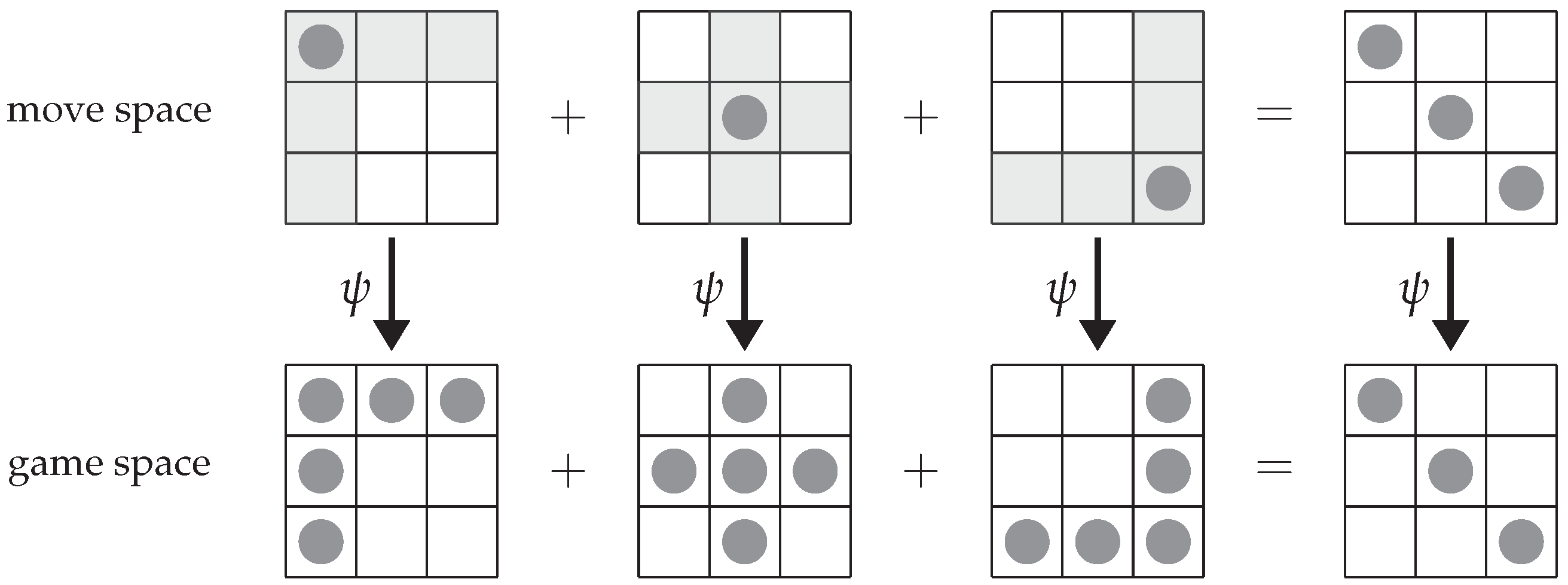
The move space, denoted by K, is the vector space over ${\mathbb{F}}_2$ spanned by the set of vectorized moves, where each vector in K corresponds to a sequence of (vectorized) moves, which is unique up to permutation. We remark that when there are totally $mn$ toggle patterns, $K=G$.

For a more general setting, the number of toggle patterns may not be $mn$, for example, the Gale–Berlekamp switching game. Although the physical meaning of “clicking” a light may not be valid, the concept of move space still works in this mathematical model. In such scenario, K may not equal to G. Yet, the remaining discussions are still valid by changing certain lengths and dimensions of the vectors and the matrices.

We can relate K and G in the following way. Define a linear map $\psi :K\to G$ that outputs a game by performing the moves stated in the input on a solved game. The image of $\psi$ is S. Being a linear map, $\psi$ is also a homomorphism. Figure 5 illustrates two examples of mapping a $k\in K$ to a $g\in G$. We can also write $\psi$ in its matrix form $\mathsf{\Psi }$, where $\mathsf{\Psi }$ is an $mn\times mn$ matrix formed by juxtaposing all vectorized toggle patterns. That is, we have $\psi \left(k\right)=\mathsf{\Psi }k$.

2.2. Linear Algebra Approach

Suppose a $k\in K$ such that $\psi \left(k\right)=s$ for some $s\in S$ is given, we can solve s by clicking the lights lit in k because $s+\psi \left(k\right)$ returns a zero vector due to the fact that subtraction is the same as addition in ${\mathbb{F}}_2$. In other words, solving a game $g\in G$ is equivalent to finding a $k\in K$ such that $\psi \left(k\right)=g$. When we represent $\psi$ in its matrix form $\mathsf{\Psi }$, we have a system of linear equations $\mathsf{\Psi }k=g$. Since $S=\left\{\psi \right(k):k\in K\}$, the dimension of the solvable game space S is the same as the dimension of the vector space spanned by the columns in $\mathsf{\Psi }$. In other words, the number of solvable games equals $2^{rank\left(\mathsf{\Psi }\right)}$.

If $\mathsf{\Psi }$ is a full rank matrix, then every game in the game space is solvable, i.e., $S=G$. Kreh [1] coined the following terminology to describe this type of game.

Definition 2

(Completely Solvable). The game is completely solvable if and only if $S=G$, i.e., every $g\in G$ is a solvable game.

We can find a sequence of moves to solve a game $g\in G$ after Gaussian elimination is applied to solve $\mathsf{\Psi }k=g$. If the number of columns in $\mathsf{\Psi }$ is more than $mn$, then some toggle patterns must be linearly dependent of some other toggle patterns. We only need to take at most $mn$ (independent) columns for finding a $k\in K$ that solves the game; hence, we can regard $\mathsf{\Psi }$ in its worst case as an $mn\times mn$ binary matrix. The problem formulation is as follows:

• Problem:  Solvability Check and/or Finding a Solution for General Two-State Lights Out Variants;
• Instance: An $mn\times 1$ binary vector $g\in G$, and an $mn\times c$ binary matrix $\mathsf{\Psi }$, with $c\le mn$;
• Question:  Is there a k that satisfies $\mathsf{\Psi }k=g$?
• Objective:  Find a k that satisfies $\mathsf{\Psi }k=g$.

As $c\le mn$, we consider the worst case $c=mn$ here. The complexity for Gaussian elimination is therefore $\mathcal{O}\left(m^3{n}^3\right)$, which is in P.

We can use Gaussian elimination to check the solvability of the game g by observing whether the solution of $\mathsf{\Psi }k=g$ exists. Other than brutally applying Gaussian elimination, there is another approach as stated in [3], which is summarized as follows: The orthogonal complement of S, denoted by $S^{\perp }$, is the null space of $\mathsf{\Psi }$. An unsolvable game, i.e., a game that is not in S, cannot be orthogonal to $S^{\perp }$. Therefore, we can determine the solvability of the game by calculating $E^{T}g$ (where each column of E corresponds to a vector in a basis of $S^{\perp }$). The game s is said to be solvable if and only if $E^{T}s=0$. In fact, this technique was also applied in coding theory for detecting errors of a linear code.

2.3. Minimal Number of Moves (The Shortest Solution)

Consider $\psi \left(k\right)=s$, i.e., the game s can be solved by the move sequence k. Based on the property of the kernel (null space) of $\psi$, as denoted by $ker\left(\psi \right)$, that $\psi \left(u\right)=0$ for all $u\in ker\left(\psi \right)$, we have $\psi (k+u)=s$ for all $u\in ker\left(\psi \right)$ due to homomorphism.

If we want to solve s with the minimal number of moves, we need to find the candidate u that minimizes the 1-norm ${\parallel k+u\parallel }_1$. This move sequence $k+u$ is then called the shortest solution of the solvable game s. If the dimension of $ker\left(\psi \right)$ is in terms of m or n, then the size of $ker\left(\psi \right)$ is exponentially large in terms of m or n; thus, an exhaustive search among all possible $u\in ker\left(\psi \right)$ is inefficient.

We now formulate the shortest solution problem for general two-state Lights Out variants (including the ordinary Lights Out). As a general problem, we need to support an arbitrary $ker\left(\psi \right)$. The dimension of the kernel is no larger than $mn$; thus, the input for describing the kernel is $mn$ amounts of $mn\times 1$ binary vectors in $ker\left(\psi \right)$ that can span the kernel. The problem is stated as follows:

• Problem:  Shortest Solution Problem for General Two-State Lights Out Variants;
• Instance:  A set B of $mn\times 1$ binary vectors in $ker\left(\psi \right)$, where $\left|B\right|=mn$ and the span of B is $ker\left(\psi \right)$, and an $mn\times 1$ binary vector $k\in K$;
• Objective:  Find a vector $u\in ker\left(\psi \right)$ that can minimize ${\parallel k+u\parallel }_1$.

Theorem 1.

The shortest solution problem for general two-state Lights Out variants is NP-hard.

Proof. 

We prove this theorem by considering the minimum distance decoding of linear code in coding theory. As a recall, the (function) problem of minimum distance decoding of a linear code is equivalent to the following: Given a parity check matrix H of the linear code and a (column vector) word k, the goal is to find out the error (column) vector e that results in the smallest Hamming weight such that $H(k-e)=0$. This is due to the property of parity check matrix that $Hc=0$ if and only if c is a codeword.

The reduction is as follows. Consider the span of the columns in H as the orthogonal complement of $ker\left(\psi \right)$, that is, every $u\in ker\left(\psi \right)$ is a codeword. Furthermore, suppose k is the move sequence that solves the game $s=\psi \left(k\right)$. Write $k=u+e$, with $u\in ker\left(\psi \right)$. Since $\psi \left(k\right)=s=\psi (k-u)=\psi \left(e\right)$, we know that e is a move sequence that can solve s. That is, by finding the shortest solution e (which has the smallest Hamming weight), we have $u=k-e\in ker\left(\psi \right)$; thus, $H(k-e)=0$. This solves the minimum distance decoding problem, and such problem is no harder than the shortest solution problem for general two-state Lights Out variants. As minimum distance decoding is NP-hard [7,8], the shortest solution problem for general two-state Lights Out variants is also NP-hard. □

Nevertheless, it is still possible to have an efficient algorithm for finding the shortest solution of a specific Lights Out variant. For example, if the game space is completely solvable, then we must have ${\parallel e\parallel }_1=0$. In such case, the move sequence obtained by the Gaussian elimination process is unique. Therefore, this problem is in P (in cubic time in terms of $mn$).

As a remark, we can also reduce this shortest solution problem to the minimum distance decoding problem in a similar manner, by treating the juxtaposition of the (column) vectors in the basis of the orthogonal complement of $ker\left(\psi \right)$ as the parity check matrix H. This shows that the two problems are actually equivalent to each other.

3. Two-State Alien Tiles

We now discuss some specific techniques for the two-state Alien Tiles problem. Note that we can regard the game space G and the solvable game space S as abelian groups under vector addition. Then, we have $S⊲G$, i.e., S is a normal subgroup of G.

Definition 3

(Syndrome). Two games have the same syndrome if and only if they are in the same coset in the quotient group $G/S$.

One crucial component that will be applied into solving our coding-theoretical problems is the function that outputs the syndrome of a game. The quotient group $G/S$ is isomorphic to the set of all syndromes.

We adopt the term “syndrome” in coding theory here because each coset represents an “error” from the solvable game space that cannot be recovered by any move sequences. In other words, an unsolvable game becomes solvable after we remove the “error” by toggling some individual lights.

3.1. Easy Games and Doubly Easy Games

For two-state Alien Tiles, we can click on any light on the game board; thus, $K=G$, i.e., the move space K equals the game space G. In other words, we can regard a game $s\in G$ as a move in K and vice versa.

Definition 4

(Easy Games). A game s is called easy if and only if it can be solved by clicking the lights lit in s, i.e., $\psi \left(s\right)=s$.

Figure 6 illustrates an example of an easy two-state Alien Tiles game. The terminology “easy” was due to Torrence [22]. In other words, s is easy if $vec\left(s\right)$ is an eigenvector of $\mathsf{\Psi }$. We also extend the terminology as follows.

Definition 5

(Doubly Easy Games). A game s is doubly easy if and only if it can be solved by first clicking the lights lit in s to obtain a game $s+\psi \left(s\right)$, then clicking the lights lit in the game $s+\psi \left(s\right)$.

That is, a game s is doubly easy if and only if:

$$s+\psi \left(s\right)+\psi (s+\psi (s\left)\right)=0.$$

Due to homomorphism and the property of binary field that $s=-s$ (i.e., s equals its additive inverse), we have:

$$s+\psi \left(s\right)+\psi (s+\psi (s\left)\right)=s+\psi (s+(s+\psi \left(s\right)\left)\right)=s+\psi \left(\psi \right(s\left)\right)=0\Rightarrow \psi \left(\psi \right(s\left)\right)=s.$$

To write down $\mathsf{\Psi }$ explicitly, we consider the following. Denote by ${𝟙}_{a,b}$ and ${𝟙}_c$ an $a\times b$ and a $c\times c$ all-ones matrix, respectively. Similarly, denote by ${\mathbf{0}}_{a,b}$ and ${\mathbf{0}}_c$ an $a\times b$ and a $c\times c$ zero matrix, respectively. Let ${\mathbf{I}}_c$ be a $c\times c$ identity matrix. By juxtaposing all (vectorized) toggle patterns, we obtain an $mn\times mn$ matrix:

$$\mathsf{\Psi }=\left(\begin{array}{ccccc}{𝟙}_m& {\mathbf{I}}_m& {\mathbf{I}}_m& \cdots & {\mathbf{I}}_m\\ {\mathbf{I}}_m& {𝟙}_m& {\mathbf{I}}_m& \cdots & {\mathbf{I}}_m\\ {\mathbf{I}}_m& {\mathbf{I}}_m& {𝟙}_m& \cdots & {\mathbf{I}}_m\\ ⋮& ⋮& ⋮& \ddots & ⋮\\ {\mathbf{I}}_m& {\mathbf{I}}_m& {\mathbf{I}}_m& \cdots & {𝟙}_m\end{array}\right)={𝟙}_n\otimes {\mathbf{I}}_m+{\mathbf{I}}_n\otimes {𝟙}_m-{\mathbf{I}}_{mn}.$$

To analyze doubly easy games, we need to apply $\psi$ multiple times on a given $k\in K$. For any positive integer c and matrix A over ${\mathbb{F}}_2$, we write $cA$ to denote $(cmod2)A$ for simplicity. In addition, note that:

$${𝟙}_c^2=\left\{\begin{array}{cc}{\mathbf{0}}_c\hfill & \mathrm{if}c\mathrm{is}\mathrm{even},\hfill \\ {𝟙}_c\hfill & \mathrm{if}c\mathrm{is}\mathrm{odd}.\hfill \end{array}\right.$$

In other words, ${𝟙}_c^2=c{𝟙}_c$. By making use of the mixed-product property of the Kronecker product:

$$(A\otimes B)(C\otimes D)=\left(AC\right)\otimes \left(BD\right)$$

where A, B, C, and D are matrices of suitable sizes that can form matrix products $AC$ and $BD$, we can now evaluate the powers of $\mathsf{\Psi }$ (over ${\mathbb{F}}_2$):

$$\begin{array}{cc}\hfill {\mathsf{\Psi }}^2& ={𝟙}_n^2\otimes {\mathbf{I}}_m+{𝟙}_n\otimes {𝟙}_m-{𝟙}_n\otimes {\mathbf{I}}_m+{𝟙}_n\otimes {𝟙}_m+{\mathbf{I}}_n\otimes {𝟙}_m^2-{\mathbf{I}}_n\otimes {𝟙}_m\hfill \\ \hfill & -{𝟙}_n\otimes {\mathbf{I}}_m-{\mathbf{I}}_n\otimes {𝟙}_m+{\mathbf{I}}_{mn}\hfill \\ \hfill & =n{𝟙}_n\otimes {\mathbf{I}}_m+m{\mathbf{I}}_n\otimes {𝟙}_m-{\mathbf{I}}_{nm},\hfill \\ \hfill {\mathsf{\Psi }}^3& =n({𝟙}_n^2\otimes {\mathbf{I}}_m+{𝟙}_n\otimes {𝟙}_m-{𝟙}_n\otimes {\mathbf{I}}_m)+m({𝟙}_n\otimes {𝟙}_m+{\mathbf{I}}_n\otimes {𝟙}_m^2-{\mathbf{I}}_n\otimes {𝟙}_m)\hfill \\ \hfill & -{𝟙}_n\otimes {\mathbf{I}}_m-{\mathbf{I}}_n\otimes {𝟙}_m+{\mathbf{I}}_{mn}\hfill \\ \hfill & =n(n-1){𝟙}_n\otimes {\mathbf{I}}_m+m(m-1){\mathbf{I}}_n\otimes {𝟙}_m-{𝟙}_n\otimes {\mathbf{I}}_m-{\mathbf{I}}_n\otimes {𝟙}_m+{\mathbf{I}}_{mn}+(m+n){𝟙}_{mn}\hfill \\ \hfill & ={𝟙}_n\otimes {\mathbf{I}}_m+{\mathbf{I}}_n\otimes {𝟙}_m-{\mathbf{I}}_{mn}+(m+n){𝟙}_{mn}\hfill \\ \hfill & =\mathsf{\Psi }+(m+n){𝟙}_{mn},\hfill \\ \hfill {\mathsf{\Psi }}^4& ={\mathsf{\Psi }}^2+(m+n)\mathsf{\Psi }{𝟙}_{mn}\hfill \\ \hfill & ={\mathsf{\Psi }}^2+(m+n)(m+n-1){𝟙}_{mn}\hfill \\ \hfill & ={\mathsf{\Psi }}^2.\hfill \end{array}$$

That is, for any positive integer $c\ge 4$, we have ${\mathsf{\Psi }}^c={\mathsf{\Psi }}^{2+(cmod2)}$.

3.2. Even-by-Even Games

When both m and n are even, we have ${\mathsf{\Psi }}^2={\mathbf{I}}_{mn}$. In other words, ${\mathsf{\Psi }}^{-1}=\mathsf{\Psi }$ and $\psi$ is an isomorphism; thus, $S=K=G$. This means that all games are solvable, i.e., every even-by-even two-state Alien Tiles is completely solvable, and the number of solvable games is $2^{mn}$.

Consider an arbitrary solvable game $s\in S$. There exists a unique $k\in K$ such that $\psi \left(k\right)=s$. Then, we have $k={\psi }^{-1}\left(s\right)=\psi \left(s\right)$, thus $\psi \left(\psi \right(s\left)\right)=s$. In other words, all solvable games are doubly easy. The size of $ker\left(\psi \right)$ is 1 as it is a zero vector space. A similar result in the case of square grids was also discussed in [23]. An interesting property of even-by-even games is the duality that $k\in K$ solves the game $s\in S$ if and only if $s\in K$ solves the game $k\in S$.

We can also view the solvability in another manner. If we know the way to toggling an arbitrary light, we can repeatedly apply this strategy to switch off the lights one by one. This also means that all games are solvable. We can toggle a single light by clicking on all the lights in the same row and the same column (where the light at the intersection of the row and the column is clicked once only). This can be observed from $\psi \left(\psi \right(s\left)\right)=s$, when s only consists of a single 1.

To compute $k={\psi }^{-1}\left(s\right)=\psi \left(s\right)$, the worst case (i.e., the case that takes the maximal number of computational steps) occurs when s is an all-ones game (a game that has all lights lit, which is an all-ones column vector of length $mn$). Every 1 in s toggles $m+n-1$ lights. Therefore, the complexity to compute k is $\mathcal{O}\left(mn(m+n-1)\right)=\mathcal{O}(m^{2}n+m{n}^2)$, which is of the same complexity as solving the linear system $\mathsf{\Psi }k=s$ directly by Gaussian elimination. On the other hand, due to the uniqueness of k, the minimal number of moves to solve s is ${\parallel k\parallel }_1={\parallel \psi \left(s\right)\parallel }_1$. To compute ${\parallel k\parallel }_1$, we scan the status of the lights after we obtain k; thus, the complexity is $\mathcal{O}(mn(m+n-1)+mn)=\mathcal{O}(m^{2}n+m{n}^2)$.

3.3. Even-by-Odd (and Odd-by-Even) Games

Due to symmetry, we only need to discuss even-by-odd games. We first discuss how to solve these games.

Note that ${\mathsf{\Psi }}^3=\mathsf{\Psi }+{𝟙}_{mn}$. For each solvable game $s\in S$, pick an arbitrary $k\in K$ such that $\psi \left(k\right)=s$. Since $\psi \left(\psi \right(\psi \left(k\right)\left)\right)=\psi \left(\psi \right(s\left)\right)$, by applying the $\psi$ map twice, we have:

$$\psi \left(\psi \left(s\right)\right)=\psi \left(k\right)+{𝟙}_{mn}k=s+{\parallel k\parallel }_1{𝟙}_{mn,1}.$$

By clicking the lit lights in s, we obtain the game $s+\psi \left(s\right)$. Afterwards, we click the lit lights in $s+\psi \left(s\right)$ to obtain the game:

$$s+\psi \left(s\right)+\psi (s+\psi \left(s\right))=s+\psi \left(\psi \left(s\right)\right)={\parallel k\parallel }_1{𝟙}_{mn,1},$$

which is either a solved game or an all-ones game.

To see how the all-ones game is being solved, we consider the following: An arbitrary row of odd length n is selected, and every light in this row is clicked. In this way, every light in this row is toggled n times, and every light not belonging to this row is toggled once. Note that $nmod2=1$; thus, every light in the game is toggled once. In other words, this move sequence can solve the all-ones game.

The (worst-case) complexity to compute $s+\psi \left(s\right)$ is $\mathcal{O}(m^{2}n+m{n}^2)$. Given $s+\psi \left(s\right)$, we have the same complexity for computing $s+\psi \left(s\right)+\psi (s+\psi (s\left)\right)$. The complexity to click every light in an arbitrary row is $\mathcal{O}\left(m{n}^2\right)$. Therefore, the overall complexity to solve a solvable game is $\mathcal{O}(m^{2}n+m{n}^2)$. We have the same complexity for finding the move sequence because the complexity for checking whether ${\parallel k\parallel }_{1}mod2=1$ is $\mathcal{O}\left(mn\right)$, which is being absorbed into $\mathcal{O}(m^{2}n+m{n}^2)$.

Next, we discuss the move sequence to toggle all the lights in an arbitrary column, which will be used in the remaining discussion. Suppose we want to toggle the j-th column. Consider this move sequence: Except the $(1,j)$-th light, click every light in the j-th column and every light in the 1-st row. Based on such operations, we have the followings:

• The $(1,j)$-th light is toggled for $m+n-2$ times, where $m+n-2$ is odd.
• Each of the other lights in the j-th column is toggled for $m-1$ times, where $m-1$ is odd.
• Each of the other lights in the 1-st row is toggled for $n-1$ times, where $n-1$ is even.
• All other lights that are not in the j-th column and not in the i-th row are toggled twice.

As a result, only the lights in the j-th column are toggled for odd number of times, then all the lights in the j-th column are being toggled.

We notice that if we apply the above move sequence to every column, the resultant move sequence is that, except the first row, all the other lights are clicked once. Although this can solve the all-ones game, this move sequence is longer than what we have previously described. This suggests that the move sequence for solving a solvable game is not unique.

We now discuss the method to check whether a game is solvable or not. Denote by $g_{ij}$ the $(i,j)$-th light in the game g. Let $r_i\left(g\right)$ be the row parity of the i-th row in g, i.e.,

$$r_i\left(g\right)=\left(\sum _{j=1}^n{g}_{ij}\right)mod2.$$

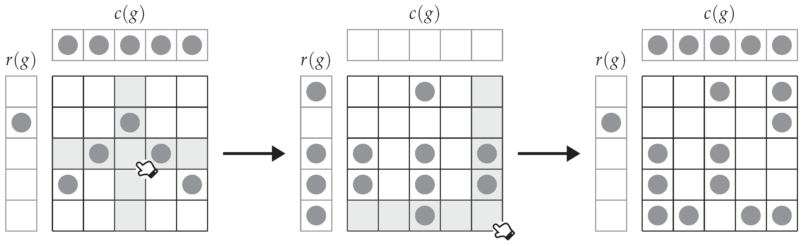
Let $r\left(g\right)={(r_1\left(g\right),r_2\left(g\right),\dots ,r_m\left(g\right))}^{⊺}$ be a column vector over ${\mathbb{F}}_2$, called the row parity vector. We can consider this row parity vector as exclusive or-ing (XOR) in all the columns, or the nim-sum of the columns.

Suppose we click an arbitrary light, say, the $(y,x)$-th light. Then, the values of $g_{ij}$ at all $i=y$ or $j=x$ are toggled. We can see that the new $r_y$ satisfies $r_y+n=r_y+1$. Except when $i=y$, the new $r_i$ will become $r_i+1$. That is, all parity bits in r are flipped. This is as illustrated in Figure 7.

To map both row parity vectors into one invariant such that any move sequence acting on a game does not change the invariant, we define the invariant function $\tilde{r}:G\to {\mathbb{F}}_2^{(m-1)\times 1}$ by:

$$\begin{array}{cc}\hfill \tilde{r}\left(g\right)& ={(r_2\left(g\right),r_3\left(g\right),\dots ,r_m\left(g\right))}^{⊺}+r_1\left(g\right){𝟙}_{m-1,1}\hfill \\ \hfill & =\left\{\begin{array}{cc}{(r_2\left(g\right),r_3\left(g\right),\dots ,r_m\left(g\right))}^{⊺}\hfill & \mathrm{if}{r}_1\left(g\right)=0,\hfill \\ {(r_2\left(g\right),r_3\left(g\right),\dots ,r_m\left(g\right))}^{⊺}+{𝟙}_{m-1,1}\hfill & \mathrm{if}{r}_1\left(g\right)=1.\hfill \end{array}\right.\hfill \end{array}$$

As every solvable game $s\in S$ gives $\tilde{r}\left(s\right)={\mathbf{0}}_{m-1,1}$, we have ${\parallel s\parallel }_{1}mod2={\parallel r\left(s\right)\parallel }_{1}mod2=0$, i.e., the number of lit lights in a solvable game is even. In addition, $\tilde{r}\left(g\right)\ne {\mathbf{0}}_{m-1,1}$ implies that the game g is not solvable. This suggests that not all games are solvable, say, a game where only the $(1,1)$-st light is lit has an invariant ${𝟙}_{m-1,1}\ne {\mathbf{0}}_{m-1,1}$.

On the other hand, any move sequence acting on a game in a coset $C\in G/S$ gives a game in the same coset, because S is the span of all toggle patterns. Then, the following question arises: What is the relation between the invariant function and the cosets? To be more specific: Does the invariant function give a syndrome of the game? The answer is affirmative.

Theorem 2.

Let g be an even-by-odd game. $\tilde{r}$ is a surjective map that maps g to its syndrome.

Proof. 

See Appendix A. □

The above theorem has the following consequences:

• $\tilde{r}\left(g\right)={\mathbf{0}}_{m-1,1}$ if and only if $g\in S$, because ${\mathbf{0}}_{m-1,1}$ is the syndrome of the solved game.
• The number of cosets in $G/S$, i.e., the index $[G:S]$, is $2^{m-1}$, due to the surjection of $\tilde{r}$.
• The number of solvable games, i.e., $\left|S\right|$, is $\left|G\right|/[G:S]=2^{mn-m+1}$.
• A game is solvable if and only if the parities of all rows are the same. The complexity of verifying the solvability is thus $\mathcal{O}\left(mn\right)$.

The method to find the minimal number of moves for solving an even-by-odd game efficiently is remained as an open problem. To justify that exhaustive search for this problem is inefficient, we calculate the size of $ker\left(\psi \right)$. By the rank-nullity theorem, we know that $dim(ker(\psi \left)\right)=m-1$. Therefore, $|ker\left(\psi \right)|=2^{m-1}$, which means that exhaustive search cannot be performed in polynomial time.

3.4. Odd-by-Odd Games

When both m and n are odd, we have ${\mathsf{\Psi }}^2=\mathsf{\Psi }$. In other words, we have $\psi \circ \psi =\psi$. For each solvable game $s\in S$, pick an arbitrary $k\in K$ such that $\psi \left(k\right)=s$. By applying $\psi$ again, we obtain $\psi \left(\psi \right(k\left)\right)=\psi \left(s\right)$. Using the fact that $\psi \left(\psi \right(k\left)\right)=\psi \left(k\right)$, we have $\psi \left(s\right)=\psi \left(k\right)=s$. That is, all solvable games are easy. Similar as the above subsections, the worst-case complexity to solve the game is $\mathcal{O}(m^{2}n+n{m}^2)$. To find a move sequence k, we only need to output s directly; thus, the complexity is $\mathcal{O}\left(mn\right)$.

To check whether a game g is solvable or not, it is insufficient to only consider the row parity vector $r\left(g\right)$. Let $c_j\left(g\right)$ be the column parity of the j-th column in g, i.e.,

$$c_j\left(g\right)=\left(\sum _{i=1}^m{g}_{ij}\right)mod2,$$

and let $c\left(g\right)=(c_1\left(g\right),c_2\left(g\right),\dots ,c_n\left(g\right))$ be a row vector over ${\mathbb{F}}_2$, called the column parity vector. When we click an arbitrary light, say, the $(y,x)$-th light, we can see that the new $r_y$ becomes $r_y+n=r_y+1$, and the new $c_x$ is $c_x+m=c_x+1$. Except when $(i,j)=(y,x)$, where the new $r_i$ is $r_i+1$ and the new $c_j$ is $c_j+1$, all the parity bits of $r\left(g\right)$ and $c\left(g\right)$ are flipped. This is as illustrated in Figure 8.

We call the pair $\left(r\right(g),c(g\left)\right)$ the parity pair of the game g. We remark that not all combinations of parity pairs are valid. The exact criteria are as stated in thm:paritydiff.

Theorem 3.

For odd-by-odd games, $g\in G$ if and only if ${\parallel r\left(g\right)\parallel }_1-{\parallel c\left(g\right)\parallel }_1$ is even.

Proof. 

We first prove the “only if” part. The result is trivial for the solved game $g={\mathbf{0}}_{mn,1}$. Consider an arbitrary non-zero game $g\in G\backslash \left\{{\mathbf{0}}_{mn,1}\right\}$. When we toggle an arbitrary lit light in g, say, the $(y,x)$-th light, to form a new game $g^{\prime }$, the row parity of the y-th row and the column parity of the x-th column are both flipped. That is, $(\parallel r\left(g^{\prime }\right){\parallel }_1-\parallel c\left(g^{\prime }\right){\parallel }_1)mod2$ equals $(\parallel r\left(g\right){\parallel }_1-\parallel c\left(g\right){\parallel }_1)mod2$. Inductively, the procedure is repeated until all lit lights are off. Then, $(\parallel r\left({\mathbf{0}}_{mn,1}\right){\parallel }_1-\parallel c\left({\mathbf{0}}_{mn,1}\right){\parallel }_1)mod2$ is equivalent to $(\parallel r\left(g\right){\parallel }_1-\parallel c\left(g\right){\parallel }_1)mod2$, where the former one equals 0. In other words, $g\in G$ implies that ${\parallel r\left(g\right)\parallel }_1-{\parallel c\left(g\right)\parallel }_1$ is even.

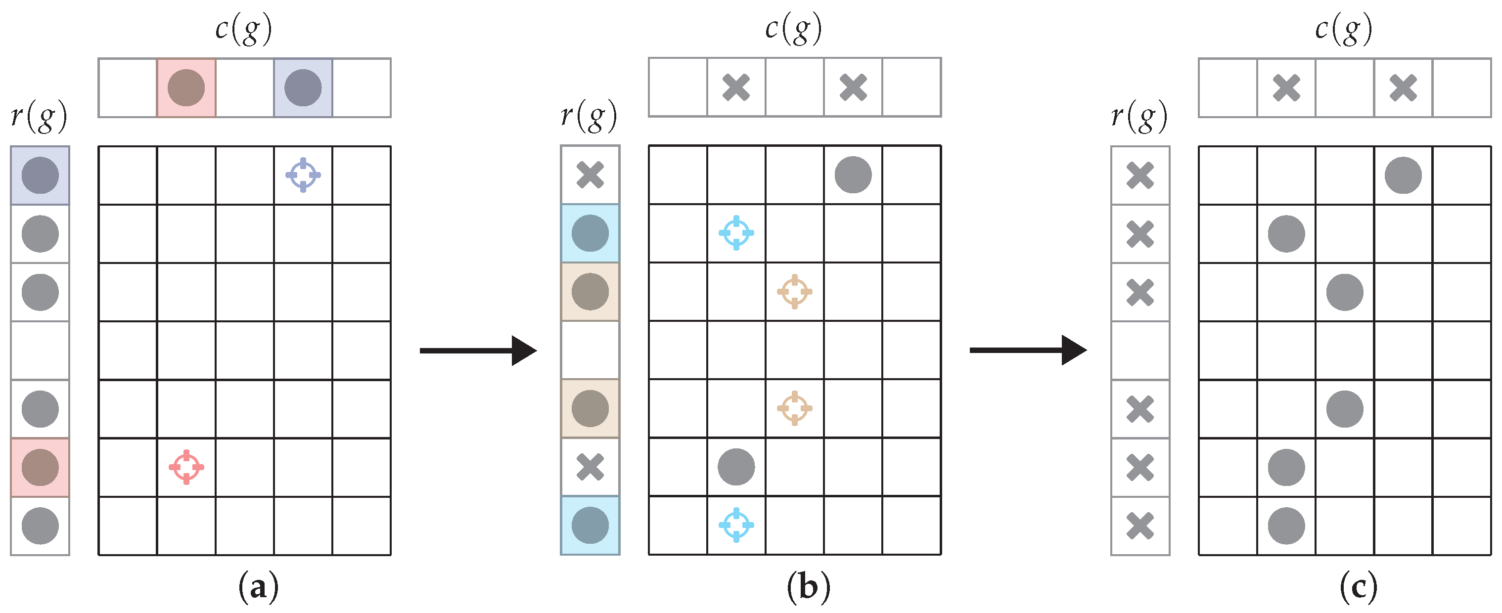
For the “if” part, we prove by construction. Let $\{y_1,y_2,\dots ,y_{{\parallel r\left(g\right)\parallel }_1}\}$ be an index set such that $r_y\left(g\right)=1$ if and only if y is in this set. Similarly, let $\{x_1,x_2,\dots ,x_{{\parallel c\left(g\right)\parallel }_1}\}$ be an index set such that $c_x\left(g\right)=1$ if and only if x is in this set.

First, we construct a game such that only the $(y_i,x_i)$-th lights are lit, where $i=1,2,\dots ,min\{\parallel r\left(g\right){\parallel }_1,\parallel c\left(g\right){\parallel }_1\}$. If ${\parallel r\left(g\right)\parallel }_1={\parallel c\left(g\right)\parallel }_1$, then the proof is done. If ${\parallel r\left(g\right)\parallel }_1>{\parallel c\left(g\right)\parallel }_1$, let $T=\{y_{{\parallel c\left(g\right)\parallel }_1+1},y_{{\parallel c\left(g\right)\parallel }_1+2},\dots ,y_{{\parallel r\left(g\right)\parallel }_1}\}$. Then, we partition T into sets of size 2, as denoted by $\left\{P_1,P_2,\dots ,P_{\frac{{\parallel r\left(g\right)\parallel }_1-{\parallel c\left(g\right)\parallel }_1}{2}}\right\}$. For every $i=1,2,\dots ,\frac{{\parallel r\left(g\right)\parallel }_1-{\parallel c\left(g\right)\parallel }_1}{2}$, let $P_i=\{a_i,b_i\}$, and we switch on the $(a_i,j)$-th and the $(b_i,j)$-th lights for an arbitrary $j\in \{1,2,\dots ,n\}$. Afterwards, the row parity vector of the game matches with $r\left(g\right)$. For each partition, we have switched on 2 lights in the same column, so the column parity of this column remains unchanged. That is, the parity pair of the resultant game is $\left(r\right(g),c(g\left)\right)$. We can prove the case ${\parallel c\left(g\right)\parallel }_1>{\parallel r\left(g\right)\parallel }_1$ in a similar manner by symmetry arguments, and the game exists in the prescribed game space. □

The construction in the above proof will also be applicable when we discuss the coding-theoretical problems. We illustrate an example of such construction in Figure 9. In this example, we start from a solved game, i.e., all lights are off. In the first phase, we match the bits in the row parity vector with the column parity vector. This example has fewer bits in the column parity vector, thus all the bits in the column parity vector are matched with some bits in the row parity vector. The bits in the row parity vector that are matched are arbitrary. In Section 3.4, the red bits are matched, followed by the blue bits. Each pair of matched bits indicates a location, which is marked by a crosshair of the same color in the game grid. By switching on the lights marked by the crosshairs, the second phase is proceeded.

The bits that are not matched must all fall into either the row or the column parity vector. In this example, there are four bits remaining in the row parity vector. We group the bits two by two arbitrarily. In Section 3.4, the two cyan bits and the two brown bits are respectively grouped. For each group, we can select an arbitrary column (if the unmatched bits fall into the column parity vector), followed by the selection of an arbitrary row. The crosshairs of the same color mark the column selected by the same group. By switching on the lights marked by the crosshairs, the desired game is constructed.

We now discuss the invariant function. Similar to the $\tilde{r}$ in even-by-odd games, we define $\tilde{c}:G\to {\mathbb{F}}_2^{1\times (n-1)}$ by:

$$\begin{array}{cc}\hfill \tilde{c}\left(g\right)& =(c_2\left(g\right),c_3\left(g\right),\dots ,c_n\left(g\right))+c_1\left(g\right){𝟙}_{1,n-1}\hfill \\ \hfill & =\left\{\begin{array}{cc}(c_2\left(g\right),c_3\left(g\right),\dots ,c_n\left(g\right))\hfill & \mathrm{if}{c}_1\left(g\right)=0,\hfill \\ (c_2\left(g\right),c_3\left(g\right),\dots ,c_n\left(g\right))+{𝟙}_{1,n-1}\hfill & \mathrm{if}{c}_1\left(g\right)=1.\hfill \end{array}\right.\hfill \end{array}$$

The invariant function for odd-by-odd games, denoted by $inv:G\to {\mathbb{F}}_2^{(m-1)\times 1}\times {\mathbb{F}}_2^{1\times (n-1)}$, is defined as:

$$inv\left(g\right)=(\tilde{r}\left(g\right),\tilde{c}\left(g\right)).$$

Again, any move sequence acting on a game will never alter the invariant. Therefore, $inv\left(g\right)\ne ({\mathbf{0}}_{m-1,1},{\mathbf{0}}_{1,n-1})$ implicates that g is not solvable. In particular, a game with only the $(1,1)$-st light lit has an invariant $({𝟙}_{m-1,1},{𝟙}_{1,n-1})\ne ({\mathbf{0}}_{m-1,1},{\mathbf{0}}_{1,n-1})$.

Unlike the case of even-by-odd games, the number of lit lights in a solvable game $s\in S$ can either be odd or even. For example, an all-ones game has odd number of lit lights, which can be solved by clicking all the lights so that every light is toggled for $m+n-1$ times, where $m+n-1$ is odd. On the other hand, a solved game is a solvable game with no lit lights, hence the number of lit lights is even.

Theorem 4.

Let g be an odd-by-odd game. inv is a surjective function that maps g to its syndrome.

Proof. 

See Appendix B. □

Similar to the discussion in the last subsection, the consequences of the above theorem include:

• $inv\left(g\right)=({\mathbf{0}}_{m-1,1},{\mathbf{0}}_{1,n-1})$ if and only if $g\in S$, because $({\mathbf{0}}_{m-1,1},{\mathbf{0}}_{1,n-1})$ is the syndrome of the solved game.
• The number of cosets in $G/S$, i.e., the index $[G:S]$, is $2^{m+n-2}$, due to the surjection of inv.
• The number of solvable games, i.e., $\left|S\right|$, is $\left|G\right|/[G:S]=2^{mn-m-n+2}$.
• A game is solvable if and only if the parities of all rows and all columns are the same. The complexity of verifying its solvability is thus $\mathcal{O}\left(mn\right)$.

Seeking an efficient algorithm to find the minimal number of moves in solving an odd-by-odd game remains an open problem nowadays. For square grids, i.e., when $n=m$, the simplified problem was discussed in [24,25], but the answers there for odd-by-odd grids are certain exhaustive searches, which have to undergo the trial of $2^{2n-2}$ possibilities, where this number equals to the size of $ker\left(\psi \right)$ for odd-by-odd square grids as discussed in [23]. For the general sense, we can easily show that $|ker\left(\psi \right)|=2^{m+n-2}$ by the rank-nullity theorem. This means that an exhaustive search on the kernel cannot be efficiently conducted.

4. Coding-Theoretical Perspective of Two-State Alien Tiles

The solvable game space S is a vector subspace of the game space G. That is, we can regard S as a linear code. Our task here is to find out the properties of S from the perspective of coding theory.

4.1. Hamming Weight

The basic parameter of an error-correcting code is the distance of the code. When the distance d is known, the error-detecting ability $d-1$ and the error-correcting ability $\lfloor \frac{d-1}{2}\rfloor$ are then obtained. As a linear code, the distance of the code equals the Hamming weight of the code, which is defined as the minimal Hamming weight among all the non-zero codewords of the code. However, finding the Hamming weight of a general linear code is NP-hard [16]. For two-state Alien Tiles, we can determine the Hamming weight of the solvable game space with ease, via the use of invariant functions.

Even-by-Even Games. These games are completely solvable, so a game with only one lit light has the minimal Hamming weight among all non-zero solvable games, i.e., the Hamming weight of such code is 1. This also means that even-by-even games have no error-detecting and correcting abilities.

Even-by-Odd Games. The syndrome of an even-by-odd solvable game is ${\mathbf{0}}_{m-1,1}$. There are two possible row parity vectors (of size $m\times 1$) that correspond to this syndrome, namely, ${\mathbf{0}}_{m,1}$ and ${𝟙}_{m,1}$.

We first consider the row parity vector ${\mathbf{0}}_{m,1}$. Each row has an even number of lit lights. As the Hamming weight of a code only considers non-zero codewords, we cannot have a row parity vector ${\mathbf{0}}_{m,1}$ for any non-zero solvable game if $n=1$. For $n>1$, the smallest ${\parallel g\parallel }_1$ equals to 2, where ${\mathbf{0}}_{mn,1}\ne g\in S$ and $r\left(g\right)={\mathbf{0}}_{m,1}$.

Now, we consider the row parity vector ${𝟙}_{m,1}$. Each row has an odd number of lit lights. That is, the smallest ${\parallel g\parallel }_1$ equals to m, where ${\mathbf{0}}_{mn,1}\ne g\in S$ and $r\left(g\right)={𝟙}_{m,1}$. As $m>0$ is even, the smallest possible m is 2. That is, we do not need to consider the row parity vector ${𝟙}_{m,1}$ unless $n=1$.

As a summary, we have:

$$\mathrm{For}\mathrm{even-by-odd}\mathrm{games},\underset{g\in S\backslash \left\{{\mathbf{0}}_{mn,1}\right\}}{min}{\parallel g\parallel }_1=\left\{\begin{array}{cc}m\hfill & \mathrm{if}n=1,\hfill \\ 2\hfill & \mathrm{otherwise}.\hfill \end{array}\right.$$

Odd-by-Odd Games. The syndrome of an odd-by-odd solvable game is the pair $({\mathbf{0}}_{m-1,1},{\mathbf{0}}_{1,n-1})$. If $m=1$, only two games are in S, which are the all-zeros and the all-ones games. Therefore, the Hamming weight of the code is n. If $n=1$, similarly, the Hamming weight is m. Both cases hold at the same time when $m=n=1$.

Now, consider the case with both m and n greater than 1, i.e., each of them is at least 3. There are two possible parity pairs (in ${\mathbb{F}}_2^{m\times 1}\times {\mathbb{F}}_2^{1\times n}$), namely, $({\mathbf{0}}_{m,1},{\mathbf{0}}_{1,n})$ and $({𝟙}_{m,1},{𝟙}_{1,n})$. For the former case, each row and each column has an even number of lit lights. In other words, the smallest ${\parallel g\parallel }_1$, where ${\mathbf{0}}_{mn,1}\ne g\in S$ and $(r\left(g\right),c\left(g\right))=({\mathbf{0}}_{m,1},{\mathbf{0}}_{1,n})$, is 4. For the latter case, each row and each column has an odd number of lit lights. That is, the minimal number of lit lights is no fewer than $max\{m,n\}$.

When $m=n$, it is easy to see that the minimal number of lit lights can be achieved by a game represented by an identity matrix. If $m\ne n$, without loss of generality, consider the case of $n>m$. An example to achieve the minimal number of lit lights $max\{m,n\}$ is the game:

$$\left(\begin{array}{cc}{\mathbf{I}}_m& \overline{)\begin{array}{c}{\mathbf{0}}_{m-1,n-m}\\ {𝟙}_{1,n-m}\end{array}}\end{array}\right).$$

Note that unless $m=n=3$, we have $max\{m,n\}\ge 5$. Therefore, we reach the conclusion that:

$$\mathrm{For}\mathrm{odd-by-oddd}\mathrm{games},\underset{g\in S\backslash \left\{{\mathbf{0}}_{mn,1}\right\}}{min}{\parallel g\parallel }_1=\left\{\begin{array}{cc}n\hfill & \mathrm{if}m=1,\hfill \\ m\hfill & \mathrm{if}n=1,\hfill \\ 3\hfill & \mathrm{if}m=n=3,\hfill \\ 4\hfill & \mathrm{otherwise}.\hfill \end{array}\right.$$

One may further combine the aforementioned results of all game sizes as follows:

$$\underset{g\in S\backslash \left\{{\mathbf{0}}_{mn,1}\right\}}{min}{\parallel g\parallel }_1=\left\{\begin{array}{cc}n\hfill & \mathrm{if}m=1,\hfill \\ m\hfill & \mathrm{if}n=1,\hfill \\ 3\hfill & \mathrm{if}m=n=3,\hfill \\ (1+(mmod2\left)\right)(1+(nmod2\left)\right)\hfill & \mathrm{otherwise}.\hfill \end{array}\right.$$

4.2. Coset Leader

The quotient group $G/S$ contains all the cosets, where each coset contains all games achieved by any possible finite move sequence from a certain setup of the game. Two games are in the same coset if and only if there exists a move sequence to transform one to another. We have discussed the technique to identify the coset that a game belongs to, mainly by finding the syndrome of the game, where each coset is associated with a unique syndrome.

Any game $g\in C\in G/S$, with $C\ne S$ being unsolvable. In the view of coding theory, we are interested in the minimal number of independent lights that we need to toggle such that the game becomes solvable. In the algebraic point of view, we want to know how far the coset C and the solvable space S are separated. That is, the mission is to find a game $e\in C$ with smallest ${\parallel e\parallel }_1$ such that $g+e\in S$. Such e can be regarded as an error, so if we know the error pattern of each coset, an error-correcting code can be applied. In coding-theoretical terminology, this e is called the coset leader of the coset C.

Even-by-Even Games. As even-by-even games have no error-correcting ability, it is not an interesting problem to find out the coset leader. In fact, we have $G/S=\left\{S\right\}=\left\{G\right\}$, and thus the coset leader of the only coset is the solved game ${\mathbf{0}}_{mn,1}$, which contains no lit lights.

Even-by-Odd Games. We consider the syndrome $\tilde{r}\left(g\right)={({\tilde{r}}_2,{\tilde{r}}_3,\dots ,{\tilde{r}}_m)}^{⊺}\in {\mathbb{F}}_2^{(m-1)\times 1}$ of a game g in a coset C. We have two possible row parity vectors, namely,

$$r={(0,{\tilde{r}}_2,{\tilde{r}}_3,\dots ,{\tilde{r}}_m)}^{⊺}\mathrm{and}{r}^{\prime }=r+{𝟙}_{m,1}.$$

First, note that the row parities of different rows are independent of each other. If the row parity of a row is 0, then there are an even number of lit lights in this row. That is, the minimal number of lit lights in this row is 0. If the row parity is 1, then there are odd number of lit lights in this row, where the minimal number is 1. In other words, the smallest ${\parallel g\parallel }_1$ such that $r\left(g\right)=r$ is ${\parallel r\parallel }_1$. The situation is similar for $r^{\prime }$.

Note that $\parallel \tilde{r}{\left(g\right)\parallel =\parallel r\parallel }_1$ and ${\parallel r\parallel }_1=m-{\parallel r^{\prime }\parallel }_1$. As both r and $r^{\prime }$ correspond to the same syndrome $\tilde{r}\left(g\right)$, we know that:

$$\underset{g\in C}{min}{\parallel g\parallel }_1={min\{\parallel r\parallel }_1,\parallel r^{\prime }{\parallel }_1\}=min\{\parallel \tilde{r}{\left(g\right)\parallel }_1,m-\parallel \tilde{r}\left(g\right){\parallel }_1\},$$

which is of time complexity $\mathcal{O}\left(m\right)$ if $\tilde{r}\left(g\right)$ is known. The coset leader is an arbitrary game that belongs to ${arg\; min}_{g\in C}{\parallel g\parallel }_1$, for example:

$$\left\{\begin{array}{cc}\left(\begin{array}{cc}\overline{)\begin{array}{c}0\\ \tilde{r}\left(g\right)\end{array}}& {\mathbf{0}}_{m,n-1}\end{array}\right)\hfill & \mathrm{if}\parallel \tilde{r}{\left(g\right)\parallel }_1\le m-\parallel \tilde{r}\left(g\right)\parallel ,\hfill \\ \left(\begin{array}{cc}\overline{)\begin{array}{c}1\\ \tilde{r}\left(g\right)+{𝟙}_{m-1,1}\end{array}}& {\mathbf{0}}_{m,n-1}\end{array}\right)\hfill & \mathrm{otherwise}.\hfill \end{array}\right.$$

The construction can be completed within $\mathcal{O}\left(mn\right)$ time. During the construction of the coset leader, if we need to put a bit in a row, we can locate it arbitrarily. Therefore, the number of coset leaders in the coset is $n^{min\{\parallel \tilde{r}\left(g\right){\parallel }_1,m-\parallel \tilde{r}\left(g\right){\parallel }_1\}}$.

Odd-by-Odd Games. Consider the syndrome $inv\left(g\right)=(\tilde{r}\left(g\right),\tilde{c}\left(g\right))$. Write $\tilde{r}\left(g\right)={({\tilde{r}}_2,{\tilde{r}}_3,\dots ,{\tilde{r}}_m)}^{⊺}$ and $\tilde{c}\left(g\right)=({\tilde{c}}_2,{\tilde{c}}_3,\dots ,{\tilde{c}}_n)$. Let

$$\overline{r}={(0,{\tilde{r}}_2,{\tilde{r}}_3,\dots ,{\tilde{r}}_m)}^{⊺}\mathrm{and}\overline{c}=(0,{\tilde{c}}_2,{\tilde{c}}_3,\dots ,{\tilde{c}}_n).$$

The syndrome can be induced by four parity pairs, namely,

$$(\overline{r},\overline{c}),(\overline{r}+{𝟙}_{m,1},\overline{c}),(\overline{r},\overline{c}+{𝟙}_{1,n})\mathrm{and}(\overline{r}+{𝟙}_{m,1},\overline{c}+{𝟙}_{1,n}).$$

According to thm:paritydiff, we know that only two out of the four parity pairs are valid, because the difference between the number of bits in the row and the column parity vectors must be an even number. Let $(r,c)$ be a valid parity pair. If the parity of a row/column is 0, then the minimal number of lit lights in this row/column is 0. If the parity is 1, then the minimal number is 1. Thus, the minimal number of lit lights is bounded below by $max\{\parallel r{\parallel }_1,\parallel c{\parallel }_1\}$.

Now, we use the construction in the proof of thm:paritydiff to construct a game $g^{\prime }$ with parity pair $(r,c)$. Note that the number of lit lights in $g^{\prime }$ is $max\{\parallel r{\parallel }_1,\parallel c{\parallel }_1\}$, which matches with the lower bound. As there are two valid parity pairs, we need to see which one results in a game that has fewer lit lights. The one with fewer lit lights is the coset leader.

The overall procedure to find out the coset leader is as follows:

• Generate $(r,c)=(\overline{r},\overline{c})$ from $inv\left(g\right)$.
• If ${\parallel r\parallel }_1-{\parallel c\parallel }_1$ is not an even number, flip all the parity bits in either r or c.
• If ${max\{m-\parallel r\parallel }_1,n-{\parallel c\parallel }_1{\}<max\{\parallel r\parallel }_1{,\parallel c\parallel }_1\}$, then flip all the parity bits in both r and c.
• Construct a game that has a parity pair $(r,c)$ (by using the construction in the proof of thm:paritydiff), and such game is denoted as the coset leader.

As we need $\mathcal{O}\left(mn\right)$ time to construct such game, the complexities of other computation steps that take either $\mathcal{O}\left(m\right)$ or $\mathcal{O}\left(n\right)$ are being absorbed by this dominant term; thus, the overall complexity to construct a coset leader is $\mathcal{O}\left(mn\right)$.

At the end of this construction, we can also obtain the minimal number of lit lights among all games in the coset, which is $max\{\parallel r{\parallel }_1,\parallel c{\parallel }_1\}$. Let

$$P=(\parallel \tilde{r}\left(g\right){\parallel }_1-\parallel \tilde{c}\left(g\right){\parallel }_1)mod2\in \{0,1\}.$$

We can also directly calculate this number as follows, with c being flipped:

$$min\left\{max\{\parallel \tilde{r}{\left(g\right)\parallel }_1,Pn+{(-1)}^P\parallel \tilde{c}{\left(g\right)\parallel }_1\},max\{m-\parallel \tilde{r}{\left(g\right)\parallel }_1,(1-P)n+{(-1)}^{1-P}\parallel \tilde{c}\left(g\right){\parallel }_1\}\right\},$$

or equivalently (flipping r):

$$min\left\{{max\{Pm+(-1)}^P\parallel \tilde{r}{\left(g\right)\parallel }_1,\parallel \tilde{c}{\left(g\right)\parallel }_1\},max\{(1-P)m+{(-1)}^{1-P}\parallel \tilde{r}{\left(g\right)\parallel }_1,n-\parallel \tilde{c}\left(g\right){\parallel }_1\}\right\}.$$

This number can be calculated in $\mathcal{O}(m+n)$ time when $inv\left(g\right)$ is given.

Let $(r^{\prime },c^{\prime })$ be the parity pair of a coset leader. We remark that the coset leader is non-unique when $\parallel r^{\prime }{\parallel }_1>1$ or $\parallel c^{\prime }{\parallel }_1>1$. Denote:

$$\alpha =max\{\parallel r^{\prime }{\parallel }_1,\parallel c^{\prime }{\parallel }_1\}\mathrm{and}\beta =min\{\parallel r^{\prime }{\parallel }_1,\parallel c^{\prime }{\parallel }_1\}.$$

To count the number of coset leaders, we recall the idea of the construction that we have used. The first phase matches each 1 in $r^{\prime }$ with a distinct 1 in $c^{\prime }$ to minimize the number of lit lights. There are totally $\left(\genfrac{}{}{0pt}{}{\alpha }{\beta }\right)\beta !$ combinations. If $\parallel r^{\prime }{\parallel }_1={\parallel c^{\prime }\parallel }_1$, then the construction is done, and the number of combinations $\left(\genfrac{}{}{0pt}{}{\alpha }{\beta }\right)\beta !=\parallel r^{\prime }{\parallel }_1!={\parallel c^{\prime }\parallel }_1!$ is achieved. Otherwise, we proceed to the second phase, which is described as follows:

The remaining unmatched 1’s must either be only in the row parity vector or only in the column parity vector. We group them two by two so that if we put each group in the same row/column, the row/column parity will not be toggled. If $\parallel r^{\prime }{\parallel }_1>{\parallel c^{\prime }\parallel }_1$, then each group can choose any of the n columns. If $\parallel c^{\prime }{\parallel }_1>{\parallel r^{\prime }\parallel }_1$, then each group can choose any of the m rows. By applying a similar technique to generate the Lagrange coefficients for Lagrange interpolation, we can combine the two cases into one formula. That is, each group has $\left(\frac{\alpha -\parallel c^{\prime }{\parallel }_1}{\parallel r^{\prime }{\parallel }_1-{\parallel c^{\prime }\parallel }_1}n+\frac{\alpha -\parallel r^{\prime }{\parallel }_1}{\parallel c^{\prime }{\parallel }_1-{\parallel r^{\prime }\parallel }_1}m\right)$ choices. It is not hard to see that we have enumerated all possibilities that can achieve the minimal number of lit lights. The number of groups is:

$$\left(\genfrac{}{}{0pt}{}{\alpha -\beta }{2}\right)\left(\genfrac{}{}{0pt}{}{\alpha -\beta -2}{2}\right)\dots \left(\genfrac{}{}{0pt}{}{2}{2}\right)=(\alpha -\beta )!2^{\frac{\beta -\alpha }{2}}.$$

Therefore, the number of possible coset leaders when $\parallel r^{\prime }{\parallel }_1\ne {\parallel c^{\prime }\parallel }_1$ is:

$$\begin{array}{cc}\hfill & \left(\genfrac{}{}{0pt}{}{\alpha }{\beta }\right)\beta !(\alpha -\beta )!2^{\frac{\beta -\alpha }{2}}\left(\frac{\alpha -\parallel c^{\prime }{\parallel }_1}{\parallel r^{\prime }{\parallel }_1-{\parallel c^{\prime }\parallel }_1}n+\frac{\alpha -\parallel r^{\prime }{\parallel }_1}{\parallel c^{\prime }{\parallel }_1-{\parallel r^{\prime }\parallel }_1}m\right)\hfill \\ \hfill =& \alpha !2^{\frac{\beta -\alpha }{2}}\left(\frac{\alpha -\parallel c^{\prime }{\parallel }_1}{\parallel r^{\prime }{\parallel }_1-{\parallel c^{\prime }\parallel }_1}n+\frac{\alpha -\parallel r^{\prime }{\parallel }_1}{\parallel c^{\prime }{\parallel }_1-{\parallel r^{\prime }\parallel }_1}m\right).\hfill \end{array}$$

Combining the two cases, the number of possible coset leaders is:

$$\left\{\begin{array}{cc}\parallel r^{\prime }{\parallel }_1!\hfill & \mathrm{if}\parallel r^{\prime }{\parallel }_1={\parallel c^{\prime }\parallel }_1,\hfill \\ \left(\genfrac{}{}{0pt}{}{\alpha }{\beta }\right)\beta !(\alpha -\beta )!2^{\frac{\beta -\alpha }{2}}\left(\frac{\alpha -\parallel c^{\prime }{\parallel }_1}{\parallel r^{\prime }{\parallel }_1-{\parallel c^{\prime }\parallel }_1}n+\frac{\alpha -\parallel r^{\prime }{\parallel }_1}{\parallel c^{\prime }{\parallel }_1-{\parallel r^{\prime }\parallel }_1}m\right)\hfill & \mathrm{otherwise}.\hfill \end{array}\right.$$

4.3. Covering Radius

The covering radius problem of the game asks for the maximal number of lights remained among all games when the player minimizes the number of lights. With the understanding of cosets, the desired number is represented by:

$$\underset{C\in G/S}{max}\underset{g\in C}{min}{\parallel g\parallel }_1.$$

Even-by-Even Games. All even-by-even games are solvable, so the covering radius is trivially 0.

Even-by-Odd Games. Recall that for each coset C,

$$\underset{g\in C}{min}{\parallel g\parallel }_1=min\{\parallel \tilde{r}{\left(g\right)\parallel }_1,m-\parallel \tilde{r}\left(g\right){\parallel }_1\}.$$

As the syndrome is a vector in ${\mathbb{F}}_2^{(m-1)\times 1}$, and each possible vector in ${\mathbb{F}}_2^{(m-1)\times 1}$ corresponds to a distinct coset, we can calculate the covering radius of even-by-odd games as follows:

$$\underset{C\in G/S}{max}\underset{g\in C}{min}{\parallel g\parallel }_1=\underset{b\in \{0,1,\dots ,m-1\}}{max}min\{b,m-b\}=\frac{m}{2}.$$

Odd-by-Odd Games. Consider a syndrome $(\tilde{r},\tilde{c})$ of a game in a coset C. Let $b=\parallel \tilde{r}{\parallel }_1$ and $a=\parallel \tilde{c}{\parallel }_1$. Each possible syndrome in ${\mathbb{F}}_2^{(m-1)\times 1}\times {\mathbb{F}}_2^{1\times (n-1)}$ corresponds to a distinct coset; therefore, it suffices to consider all possible $b\in \{0,1,\dots ,m-1\}$ and $a\in \{0,1,\dots ,n-1\}$. Note that we are considering the syndrome but not the parity pair, and therefore $a-b$ can either be even or odd.

Case I: $a-b$ is even. Then, we have:

$$\underset{g\in C}{min}{\parallel g\parallel }_1=min\{max\{b,a\},max\{m-b,n-a\}\}.$$

To maximize this number among all cosets, we need to check both $(b,a)=(0,n-1)$ and $(b,a)=(m-1,0)$, which gives $min\{n-1,m\}$ and $min\{m-1,n\}$, respectively. That is, if we restrict ourselves to those $a-b$ that are even, the covering radius is:

$$max\{min\{n-1,m\},min\{m-1,n\}\}=min\{m,n\}-{\delta }_{m,n},$$

where ${\delta }_{m,n}$ is the Kronecker delta, i.e.,

$${\delta }_{m,n}=\left\{\begin{array}{cc}1\hfill & \mathrm{if}m=n,\hfill \\ 0\hfill & \mathrm{otherwise}.\hfill \end{array}\right.$$

Case II: $a-b$ is odd. Then, we have:

$$\underset{g\in C}{min}{\parallel g\parallel }_1=min\{max\{b,n-a\},max\{m-b,a\}\}.$$

To maximize this number among all cosets, we need to check both $(b,a)=(1,0)$ and $(b,a)=(0,1)$, which gives $min\{n,m-1\}$ and $min\{n-1,m\}$, respectively. That is, if we restrict ourselves to those $a-b$ that are odd, the covering radius is $max\{min\{n,m-1\},min\{n-1,m\left\}\right\}$, which is the same as when $a-b$ is even.

Combining these two cases, the covering radius of odd-by-odd games can be represented as:

$$\underset{C\in G/S}{max}\underset{g\in C}{min}{\parallel g\parallel }_1=min\{m,n\}-{\delta }_{m,n}.$$

4.4. Error Correction

The error correction problem is to find a solvable game by toggling the fewest number of lights individually. Depending on the capability of error correcting, such a corrected game may not be unique.

Even-by-Even Games. All even-by-even games are solvable; therefore, there is no unsolvable game for discussion.

Even-by-Odd Games. When $n>1$, the Hamming distance is 2. Thus, the code has single error-detecting ability, but with no error-correcting ability.

When $n=1$, the Hamming distance is an even number. Denote such even number as m. Thus, the code has $\left(m-1\right)$ error-detecting ability and $\lfloor \frac{m-1}{2}\rfloor =\frac{m}{2}-1$ error-correcting ability. Note that an $m\times 1$ game only consists of two codewords, namely, ${\mathbf{0}}_{m,1}$ and ${𝟙}_{m,1}$.

Consider an arbitrary vector $w\in {\mathbb{F}}_2^{m\times 1}$. If there are $\frac{m}{2}$ number of 0’s and $\frac{m}{2}$ number of 1’s in w, then we cannot correct the error because the Hamming distance from w to either of the codewords is the same. If the number of 0’s in w is more than that of 1’s, then w is closer to ${\mathbf{0}}_{m,1}$. If the number of 1’s in w is more than that of 0’s, then w is closer to ${𝟙}_{m,1}$. In the latter two cases, the number of errors is at most $\frac{m}{2}-1$; thus, the closest solvable game is unique. In fact, this code is known as a repetition code in coding theory.

Odd-by-Odd Games. When $m>1$ and $n=1$, the code is again a repetition code as previously mentioned. However, in this context, m is an odd number; therefore, the code has $\frac{m-1}{2}$ error-correcting ability.

Consider an arbitrary vector $w\in {\mathbb{F}}_2^{m\times 1}$. It is impossible to have the same number of 0’s and 1’s in w. Therefore, we can always correct w to the closest solvable game and such a solvable game is unique. A similar result holds for $m=1$ and $n>1$ based on symmetry. However, when $m=n=1$, the Hamming distance is 1, thus, the code has no error-detecting nor error-correcting abilities.

The non-trivial cases are the odd-by-odd games when $m,n>1$. Suppose we have an unsolvable odd-by-odd game $g\in G\backslash S$. We first calculate the syndrome $inv\left(g\right)$ to identify the coset that the game g belongs to. Then, we find an arbitrary coset leader e of such coset. Recall that the coset leader of a coset is the game that has the minimal number of lit lights. Therefore, the game $g-e$ is a closest solvable game.

The code distance of a $3\times 3$ game is 3; thus, it has 2 error-detecting abilities and 1 error-correcting ability. For games of any other size, the distance is 4; therefore, the code has 3 error-detecting abilities and 1 error-correcting ability. This also implies that for any unsolvable odd-by-odd game $g\in G\backslash S$, the closest solvable game is unique if and only if the coset leader of the coset where the game it belongs to has one and only one lit light.

In principle, we can use the syndrome of the game to directly locate the error when there is only 1 error. The procedure is as follows:

• Calculate the syndrome $inv\left(g\right)=({({\tilde{r}}_2,{\tilde{r}}_3,\dots ,{\tilde{r}}_m)}^{⊺},({\tilde{c}}_2,{\tilde{c}}_3,\dots ,{\tilde{c}}_n))$ of the given game g;
• Initialize $r={(0,{\tilde{r}}_2,{\tilde{r}}_3,\dots ,{\tilde{r}}_m)}^{⊺}$, $c=(0,{\tilde{c}}_2,{\tilde{c}}_3,\dots ,{\tilde{c}}_n)$, $A={\parallel r\parallel }_1$, and $B={\parallel c\parallel }_1$;
• If $A-B$ is odd, then let $A=m-{\parallel r\parallel }_1$ and flip all the bits in r;
• If $max\{A,B\}=0$ or $max\{m-A,n-B\}=0$, then the game g is already solvable, and this procedure is then completed;
• If $max\{A,B\}>1$ and $max\{m-A,n-B\}>1$, then there is more than one error, which implicates that the errors cannot be uniquely corrected. Therefore, the procedure can again be terminated;
• If $max\{A,B\}>max\{m-A,n-B\}$, then flip all the bits in both vectors r and c;
• Let y and x be the indices where the y-th entry in r is 1 and the x-th entry in c is 1. Then, the $(y,x)$-th light in g is the only error position.

The idea of the above procedure is similar to the construction of the coset leader. We first find a valid parity pair of g, i.e., $A-B$ is even. Next, we filter out the cases where the game has no errors, or has more than one error. If $1=max\{A,B\}\le max\{m-A,n-B\}$, then the current parity pair has exactly one 1 in each of the row and column parity vectors. Otherwise, we have $max\{m-A,n-B\}=1$; then, we flip both the row and column parity vectors such that there is exactly one 1 in both parity vectors. As a result, the coset leader has exactly one 1 in this case, where the location of the 1 is indicated by the parity pair.

5. As an Error-Correcting Code

In this section, we discuss the use of the solvable game space of a two-state Alien Tiles game as an error-correcting code. Although the general linear code technique based on the generator matrix and the parity check matrix also work, the corresponding matrices have a much more complicated form. Here, we describe a natural and simple way for encoding and decoding. We also discuss whether the code is an optimal linear code or not, where optimality means that the linear code has the maximal number of codewords among all possible linear codes under the same set of parameters, for example, field size, codeword length, and code distance.

5.1. Even-by-Odd Games

We first discuss the $m\times 1$ games. An $m\times 1$ game only consists of two codewords, namely, ${\mathbf{0}}_{m,1}$ and ${𝟙}_{m,1}$, so it is simply a repetition code. The message that we can encode is either the bit 0 or 1. To encode, we simply map 0 to ${\mathbf{0}}_{m,1}$ and map 1 to ${𝟙}_{m,1}$. The way to decode was discussed in the last section, which is precisely described as follows: Let $a,b\in \{0,1\}$, where $a\ne b$. If the number of a’s in a to-be-decoded word is more than that of b’s, then we decode to a. If their numbers are equal, then we cannot uniquely decode the word.

Now, consider $n>1$. All these games have single error-detecting ability but no error-correcting abilities, because the code distance is 2. As the size of the solvable game space, i.e., the number of codewords, is $\left|S\right|=2^{mn-m+1}$, we have $mn-(mn-m+1)=m-1$ bits acting as the redundancy for error detection. The message that we can encode is an $\left(mn-m+1\right)$-bits string. Denote the message by $(b_1,b_2,\dots ,b_{mn-m+1})$, a natural way to encode the message is as follows: We first consider an $m\times (n-1)$ matrix:

$$D=\left(\begin{array}{cccc}{b}_1& b_2& \cdots & b_{n-1}\\ b_n& b_{n+1}& \cdots & b_{2n-2}\\ ⋮& ⋮& \ddots & ⋮\\ b_{mn-m-n+2}& b_{mn-m-n+3}& \cdots & b_{mn-m}\end{array}\right)$$

and calculate its row parity vector $r={(r_1,r_2,\dots ,r_m)}^{⊺}$. If $b_{mn-m+1}=r_1$, then we construct the game:

$$\left(\begin{array}{cc}r& D\end{array}\right).$$

Otherwise, we construct the game:

$$\left(\begin{array}{cc}r+{𝟙}_{m,1}& D\end{array}\right).$$

The row parity vector of the former game is ${\mathbf{0}}_{m,1}$, and the one of the latter game is ${𝟙}_{m,1}$. That is, both games are solvable. Thus, we have encoded the message.

Note that the $(1,1)$-st entry of the encoded message is the same as $b_{mn-m+1}$. Therefore, we can perform the following steps to decode a game g:

• Calculate the row parity vector $r\left(g\right)$ of the game g.
• If $r\left(g\right)\ne {\mathbf{0}}_{m,1}$ and $r\left(g\right)\ne {𝟙}_{m,1}$, then we have detected the existence of errors, but we cannot decode the game; thus, the decoding procedure can be terminated.
• The game has no errors; thus, the message can be recovered by referring to the matrix.

Lastly, we discuss the optimality of the code. The optimality of $m\times 1$ games follows the optimality of repetition codes, which can easily be verified by the use of the Singleton bound [26].

Theorem 5.

For even-by-odd games (where $n>1$), only the $2\times n$ games are optimal linear codes.

Proof. 

We first consider $m=2$. Recall that $\left|S\right|=2^{2n-1}$. By applying the Singleton bound [26], we have:

$$A_2(2n,2)\le 2^{2n-2+1}=2^{2n-1},$$

where $A_q(\ell ,d)$ denotes the maximal number of codewords among all possible linear or non-linear codes with field size q, codeword length ℓ, and code distance d. As $A_2(2n,2)=\left|S\right|$, we know that all $2\times n$ games are optimal linear codes.

Now, we consider $m>2$. If there exists a linear code having the same set of parameters, but of a greater number of codewords, we can conclude that the error-correcting code (ironically without error-correcting ability) formed by even-by-odd games (with $n>1$) is not an optimal linear code. The existence of such code is shown by the following construction. Consider $D={\mathbb{F}}_2^{mn-1}$, where $mn-1$ is odd. Take any two arbitrary $a,b\in D$ such that their Hamming distance is 1. One of them has odd number of bits and the other has even number of bits. Without loss of generality, assume a has an odd number of bits. We append a parity bit, i.e., 1, at the end of a, and append a parity bit, i.e., 0, at the end of b. The extended words (vectors) are elements in ${\mathbb{F}}_2^{mn}$, and their Hamming distance is 2. That is, by appending a parity bit to every word in D, we obtain a linear code that has the same set of parameters as the even-by-odd games when $n>1$. The number of codewords is $2^{mn-1}$, which is greater than $\left|S\right|=2^{mn-m+1}$. This proves the non-optimality of even-by-odd games, with $m>2$ and $n>1$. □

5.2. Odd-by-Odd Games

When $m=1$ or $n=1$ (but not both), the code is an repetition code; thus, it is optimal. The way to encode and decode is similar to that of even-by-1 games, except that the numbers of 0’s and 1’s are never the same. If $m=n=1$, then there is no unsolvable game. Thus, we do not need to consider this case.

In the remaining discussion of this sub-section, we only consider odd-by-odd games, with $m,n\ge 3$.

Theorem 6.

For odd-by-odd games (where $m,n\ge 3$), only the $3\times 3$ games form an optimal linear code.

Proof. 

See Appendix C. □

Recall that for all $3\times 3$ games, the Hamming distance of this code is 3. Thus, it is 2 error-detecting and 1 error-correcting. For games of larger sizes, i.e., $m,n\ge 3$ but not $m=n=3$, their Hamming distances are all 4. Thus, they are 3 error-detecting and 1 error-correcting. That is, we can only correct up to one error. Regardless of the optimality, we now discuss the natural way to encode and decode.

The dimension of the solvable game space is $mn-m-n+2$; thus, the message that we can encode is an $\left(mn-m-n+2\right)$-bits string. Denote the message by $(b_1,b_2,\dots ,b_{mn-m-n+2})$. First, we put the message into a matrix in the form:

$$\left(\begin{array}{cc}{b}_{mn-m-n+2}& {\mathbf{0}}_{1,n-1}\\ {\mathbf{0}}_{m-1,1}& D\end{array}\right)\mathrm{where}D:=\left(\begin{array}{cccc}{b}_1& b_2& \cdots & b_{n-1}\\ b_n& b_{n+1}& \cdots & b_{2n-2}\\ ⋮& ⋮& \ddots & ⋮\\ b_{mn-m-2n+3}& b_{mn-m-2n+4}& \cdots & b_{mn-m-n+1}\end{array}\right).$$

Let $(r,c)$ be the parity pair of D. By thm:paritydiff, the number of bits in r and c must either be both odd or both even. If the number of bits in r (or c) is even, then the game

$$\left(\begin{array}{cc}0& c\\ r& D\end{array}\right)$$

has a parity pair $({\mathbf{0}}_{m,1},{\mathbf{0}}_{1,n})$. If the number of bits in r (or c) is odd, then the game

$$\left(\begin{array}{cc}1& c\\ r& D\end{array}\right)$$

has a parity pair $({\mathbf{0}}_{m,1},{\mathbf{0}}_{1,n})$. In both of the above games, if the $(1,1)$-st entry is not equal to $b_{mn-m-n+2}$, then we click the $(1,1)$-st light so that all the lights in the first row and the first column are toggled. Combining these two cases,

Table 1. The condition to flip all the bits in the parity pair $(r,c)$ for encoding a message to an odd-by-odd game, where $m,n\ge 3$.

${\parallel \mathit{r}\parallel }_{1}mod2$ (or ${\parallel \mathit{c}\parallel }_{1}mod2$)	${\mathit{b}}_{\mathbf{mn}-\mathit{m}-\mathit{n}+2}$	Flip?
0	0	No
0	1	Yes
1	0	Yes
1	1	No

shows the condition to flip all the bits in the parity pair.

The table is actually the truth table of exclusive OR (XOR). As addition in binary field is equivalent to modulo 2 addition, we can write the desired codeword as:

$$\left(\begin{array}{cc}{b}_{mn-m-n+2}& c+{(\parallel c\parallel }_1+b_{mn-m-n+2}){𝟙}_{1,n-1}\\ r+{(\parallel r\parallel }_1+b_{mn-m-n+2}){𝟙}_{m-1,1}& D\end{array}\right).$$

To decode a game, we can run the procedure as described in Section 4.4. The procedure has three types of output:

• The first type of output indicates the game is a solvable one. Therefore, we can directly extract the message $(b_1,b_2,\dots ,b_{mn-m-n+2})$.
• The second type of output indicates the game has more than one error, so the error correction is non-unique. Thus, we consider the code as non-decodable.
• The third type of output indicates the location of the single error. Let $(y,x)$ be the location of the error, we can correct the error by flipping the $(y,x)$-th bit of the game grid.

5.3. Example

To demonstrate the error-correcting code, we provide an example in this sub-section. Consider the $3\times 3$ games. Suppose we want to encode the message $(1,1,0,1,0)$. First, the matrix D that consists of the first four bits of the message is:

$$D=\left(\begin{array}{cc}1& 1\\ 0& 1\end{array}\right).$$

Then, we fill in the parity pair of D, which is $(r,c)=({(0,1)}^{⊺},(1,0))$, to a $3\times 3$ game:

$$\left(\begin{array}{ccc}0& 1& 0\\ 0& 1& 1\\ 1& 0& 1\end{array}\right).$$

As ${\parallel r\parallel }_{1}mod2=1$ and the last bit of the message is 0, according to Table 1, we need to flip the first row and the first column except the $(1,1)$-st entry. Thus, the encoded codeword is:

$$\left(\begin{array}{ccc}0& 0& 1\\ 1& 1& 1\\ 0& 0& 1\end{array}\right).$$

Now, we introduce an error to the codeword. Note that the error can be located at any entry in the codeword, including those bits that are not the message bits. For example, the erroneous codeword is:

$$w=\left(\begin{array}{ccc}0& 0& 1\\ 0& 1& 1\\ 0& 0& 1\end{array}\right).$$

To correct such error, we first calculate the syndrome of this game, which is $({(1,0)}^{⊺},(1,1))$. Next, we initialize $r={(0,1,0)}^{⊺}$ and $c=(0,1,1)$. As ${\parallel r\parallel }_1-{\parallel c\parallel }_1=-1$ is odd, we flip the bits in r. Thus, r becomes ${(1,0,1)}^{⊺}$. Now, we have:

$$2={max\{\parallel r\parallel }_1{,\parallel c\parallel }_1\}>max\{3-{\parallel r\parallel }_1,3-{\parallel c\parallel }_1\}=1,$$

so we flip both r and c. That is, we have $r={(0,1,0)}^{⊺}$ and $c=(1,0,0)$. This pair of bits indicates that the error is located at:

$$e=\left(\begin{array}{ccc}0& 0& 0\\ 1& 0& 0\\ 0& 0& 0\end{array}\right).$$

Afterwards, we can correct the error by $w-e$ and obtain the codeword

$$\left(\begin{array}{ccc}0& 0& 1\\ 1& 1& 1\\ 0& 0& 1\end{array}\right).$$

By directly reading this matrix, the decoded message $(1,1,0,1,0)$ can be recovered.

6. States Decomposition

One may wonder whether we can practically decompose the four states of the ordinary (four-state) Alien Tiles to obtain two two-state Alien Tiles games. We describe a states decomposition method below, where the number of states and the toggle patterns can be arbitrary. Suppose there are q states. We reuse $\mathsf{\Psi }$ to denote the matrix of all vectorized toggle patterns. Suppose q has P distinct prime factors. We can express q in canonical representation:

$$q=\prod _{i=1}^P{p}_i^{r_i}$$

where $p_i$ are distinct primes.

To show whether the (vectorized) game g is solvable, it is equivalent to show whether the linear system

$$\mathsf{\Psi }k\equiv g(modq)$$

is solvable. By applying the Chinese remainder theorem, we can decompose the system into

$$\left\{\begin{array}{c}\mathsf{\Psi }k\equiv g(mod{p}_1^{r_1})\hfill \\ \mathsf{\Psi }k\equiv g(mod{p}_2^{r_2})\hfill \\ ⋮\hfill \\ \mathsf{\Psi }k\equiv g(mod{p}_P^{r_P})\hfill \end{array}\right.$$

and combine the solutions of the above system into a unique modulo q solution afterwards. Our task becomes solving the linear system in the form of:

$$\mathsf{\Psi }k\equiv g(mod{p}^r)$$

(1)

where p is a prime. If $r=1$, we cannot further decompose the system, which means that we have to directly solve the problem.

Consider $r\ge 2$. The solution of Equation (1) is also a solution of the linear system

$$\mathsf{\Psi }k\equiv g(modp).$$

Let $k_0$ be a solution of this system. We have:

$$\mathsf{\Psi }{k}_0-g=pz$$

for some integer vector z (after vectorization). Let $k_0+py$ be a solution of Equation (1). We have:

$$\begin{array}{cc}\hfill \mathsf{\Psi }(k_0+py)-g& \equiv 0(mod{p}^r)\hfill \\ \hfill (\mathsf{\Psi }{k}_0-g)+p\mathsf{\Psi }y& \equiv 0(mod{p}^r)\hfill \\ \hfill pz+p\mathsf{\Psi }y& \equiv 0(mod{p}^r).\hfill \end{array}$$

By dividing p, we obtain:

$$\mathsf{\Psi }y\equiv -z(mod{p}^{r-1}).$$

Repeatedly applying this procedure, we can reduce the power of the prime in the modulo until $r=1$.

The main issue of this decomposition is that the solution $k_0$ may not be unique. We need to try which $k_0+u$ is solvable after we reduce the prime power, where $\mathsf{\Psi }umodp$ is equivalent to a zero game. A wrong choice can lead to an unsolvable system. This also happens when we reduce the four-state Alien Tiles to the two-state ones.

However, if m and n are both even, all four-state Alien Tiles games are solvable [4,21]. In other words, the move sequence to solve an arbitrary game is unique (up to permutation). We do not need to concern the choice of $k_0$ as every even-by-even two-state Alien Tiles is solvable. A summary of the procedures in solving a four-state Alien Tiles g by states decomposition is as follows:

• Find a move sequence k that solves the two-state Alien Tiles $gmod2$.
• Calculate $z=\frac{1}{2}(\mathsf{\Psi }k-g)$ without performing modulo.
• Find a move sequence y that solves the two-state Alien Tiles $zmod2$.
• The move sequence in solving the four-state Alien Tiles g is $k+2y$.

As an example, consider the four-state Alien Tiles:

$$g=\left(\begin{array}{cccc}0& 0& 0& 0\\ 0& 1& 2& 0\\ 0& 3& 0& 0\\ 0& 0& 0& 0\end{array}\right)$$

where the four states are mapped to 0, 1, 2, and 3, respectively. The first step is to solve the two-state game:

$$gmod2=\left(\begin{array}{cccc}0& 0& 0& 0\\ 0& 1& 0& 0\\ 0& 1& 0& 0\\ 0& 0& 0& 0\end{array}\right).$$

The move sequence is

$$k=\left(\begin{array}{cccc}0& 0& 0& 0\\ 1& 0& 1& 1\\ 1& 0& 1& 1\\ 0& 0& 0& 0\end{array}\right).$$

Next, we calculate:

$$z=\frac{1}{2}(\mathsf{\Psi }k-g)=\frac{1}{2}\left(\left(\begin{array}{cccc}2& 0& 2& 2\\ 0& 3& 0& 0\\ 0& 3& 0& 0\\ 2& 0& 2& 2\end{array}\right)-\left(\begin{array}{cccc}0& 0& 0& 0\\ 0& 1& 2& 0\\ 0& 3& 0& 0\\ 0& 0& 0& 0\end{array}\right)\right)=\left(\begin{array}{cccc}1& 0& 1& 1\\ 0& 1& -1& 0\\ 0& 0& 0& 0\\ 1& 0& 1& 1\end{array}\right).$$

After that, we solve another two-state game:

$$zmod2=\left(\begin{array}{cccc}1& 0& 1& 1\\ 0& 1& 1& 0\\ 0& 0& 0& 0\\ 1& 0& 1& 1\end{array}\right).$$

The move sequence is:

$$y=\left(\begin{array}{cccc}0& 0& 1& 0\\ 0& 0& 0& 0\\ 0& 1& 1& 0\\ 0& 0& 1& 0\end{array}\right).$$

Finally, we obtain the move sequence that solves the four-state game g, which is:

$$k+2y=\left(\begin{array}{cccc}0& 0& 2& 0\\ 1& 0& 1& 1\\ 1& 2& 3& 1\\ 0& 0& 2& 0\end{array}\right).$$

7. Conclusions

The study of Lights Out and its variants is mostly for theoretical interests and pedagogical purposes. The main goals and purposes of this paper are to stimulate the interests of the recreational mathematics community in investigating special features of switching games, apart from dealing with the solvability problems. Furthermore, this study can provide an entry point for recreational mathematicians to easily pick up and explore related switching game problems, even though they may not excel in coding theory and related mathematical disciplines.

In this paper, we investigated the properties of two-state Alien Tiles, including the solvability, invariants, etc., based on different settings. We also discussed the efficient methods to deal with coding-theoretical problems for the game, such as the Hamming weight, the coset leader, and the covering radius. We also demonstrated how to apply the game as an error-correcting code with a natural way to encode and decode and verified that particular game sizes can form optimal linear codes. An open problem that remains in this paper is the existence of an efficient method to find out the minimal number of moves (the shortest solution) in solving a solvable game. Lastly, we discussed the states decomposition method and left an open problem on the issue of kernel selection.

One future direction is to study the coding-theoretical problems on the ordinary Lights Out and also its other variants. Different variants possess different structures and have to be explored in depth. In particular, some variants may have easy solutions, e.g., the two-state Alien Tiles that we have discussed in this paper; while some of them may not, e.g., the Gale–Berlekamp switching game. In addition to constructing easy solutions, proving how hard a game problem is will also be a potential research direction.

Another future direction is to investigate more structural properties of the ordinary four-state Alien Tiles. In the four-state version, there is a subtle issue when we model the problem via the use of linear algebra. Take the odd-by-odd games as an example: We can click all the lights twice in a) two arbitrary distinct columns, b) two arbitrary distinct rows, or c) an arbitrary column, followed by an arbitrary row, to keep an arbitrary game unchanged. The combination of these actions forms a kernel. As each light must be clicked for even number of times, the kernel is a free module instead of a vector space over ${\mathbb{F}}_4$, which means that it is a module that has a basis. This is because multiplication in this finite field is not having the same effect as taking modulo after integer multiplication. In particular, applying two double clicks is equivalent to “no clicking”; however, $2\times 2\ne 0$ in ${\mathbb{F}}_4$.

On top of this, we have concluded that the states decomposition has an issue in finding a proper element in the kernel that leads to a solvable game in the lower state. However, this also means that we have reduced the search space by eliminating those elements in the kernel that lead to an unsolvable game in the lower state. A future direction is to investigate whether this decomposition can help in solving constraint programming problems like that described in [27]. This problem is a recreational mathematics problem on Alien Tiles, which aims to find the solvable game that has the longest “shortest solution ”. Existing approaches reduce the search space mainly by symmetry breaking [28,29,30]. The use of our states decomposition together with symmetry breaking in obtaining desired solvable games (which may not be unique) is a potential research direction.