Article

Enhancing the Transferability of Adversarial Examples with Feature Transformation

1
School of Artificial Intelligence and Computer Science, Jiangnan University, Wuxi 214122, China
2
Jiangsu Provincial Engineering Laboratory of Pattern Recognition and Computational Intelligence, Jiangnan University, Wuxi 214122, China
*
Author to whom correspondence should be addressed.
Mathematics 2022, 10(16), 2976; https://doi.org/10.3390/math10162976
Submission received: 26 July 2022 / Revised: 16 August 2022 / Accepted: 17 August 2022 / Published: 18 August 2022

Abstract

:
The transferability of adversarial examples allows the attacker to fool deep neural networks (DNNs) without knowing any information about the target models. The current input transformation-based method generates adversarial examples by transforming the image in the input space, which implicitly integrates a set of models by concatenating image transformation into the trained model. However, the input transformation-based methods ignore the manifold embedding and hardly extract intrinsic information from high-dimensional data. To this end, we propose a novel feature transformation-based method (FTM), which conducts feature transformation in the feature space. FTM can improve the robustness of adversarial example by transforming the features of data. Combining with FTM, the intrinsic features of adversarial examples are extracted to generate transferable adversarial examples. The experimental results on two benchmark datasets show that FTM could effectively improve the attack success rate (ASR) of the state-of-the-art (SOTA) methods. FTM improves the attack success rate of the Scale-Invariant Method on Inception_v3 from 62.6% to 75.1% on ImageNet, which is a large margin of 12.5%.

1. Introduction

DNNs have been shown to perform well in many fields, for example, image classification [1,2,3], human recognition [4], image segmentation [5], image fusion [6], visual object tracking [7,8], super-resolution [9], etc [10]. The ultimate goal of these studies is to make DNN-based applications more practicable and efficient. However, the existence of adversarial examples presents a concern for security of many applications, such as autonomous driving [11], face recognition [12,13,14], etc.
Adversarial examples [15], generated by adding indistinguishable perturbations to the raw images, can lead the DNNs to make completely different predictions. They can even take effect for completely unknown models, which is called the transferability of adversarial examples. In addition to this, there are several studies on universal adversarial perturbations [16,17], which are able to take effect on any image. Some studies are devoted to the application of adversarial examples to real-world scenarios, such as face recognition, autonomous driving, etc. [18,19,20,21,22]. Studying both adversarial attack and defense [23,24,25,26] is of significance, not only in revealing the vulnerability of DNNs, but also in improving the robustness of DNNs.
Many white-box attack methods have been proposed, such as Fast Gradient Sign Method (FGSM) [27], Basic Iterative Method (BIM) [28], etc. However, it is difficult for an attacker to obtain the structure and other parameters of the target model in the real-world situation. Therefore, various approaches have emerged to enhance the transferability of adversarial examples for black-box attack. Ensemble Attack [29] is an effective method to enhance the transferability of adversarial examples. Lin et al. [30] proposed Scale-Invariant Method (SIM), which utilizes input transformation to obtain a new model. A set of models can be obtained by using different transformations several times. With this approach, they can perform an ensemble attack with only one trained model, which is an implicit ensemble attack. Input transformation-based methods are successfully used for an adversarial attack, such as Diverse Input Method (DIM) [31], Translation-Invariant Method (TIM) [32], Admix Attack Method (Admix) [33], etc. However, these methods ignore the manifold structure of adversarial examples and few works focus on feature transformation. To this end, this work proposes a feature transformation-based method (FTM) to improve the transferability of adversarial examples. Compared with the input transformation, our approach transforms the intrinsic features of data instead of the input images. FTM is an implicit ensemble attack that can simultaneously attack multiple models that extract different features. It can improve the robustness of the adversarial example at the feature level. This work proposes several feature transformation strategies. FTM could effectively improve the performance of the SOTA adversarial attacks. Our contributions can be summarized as follows.
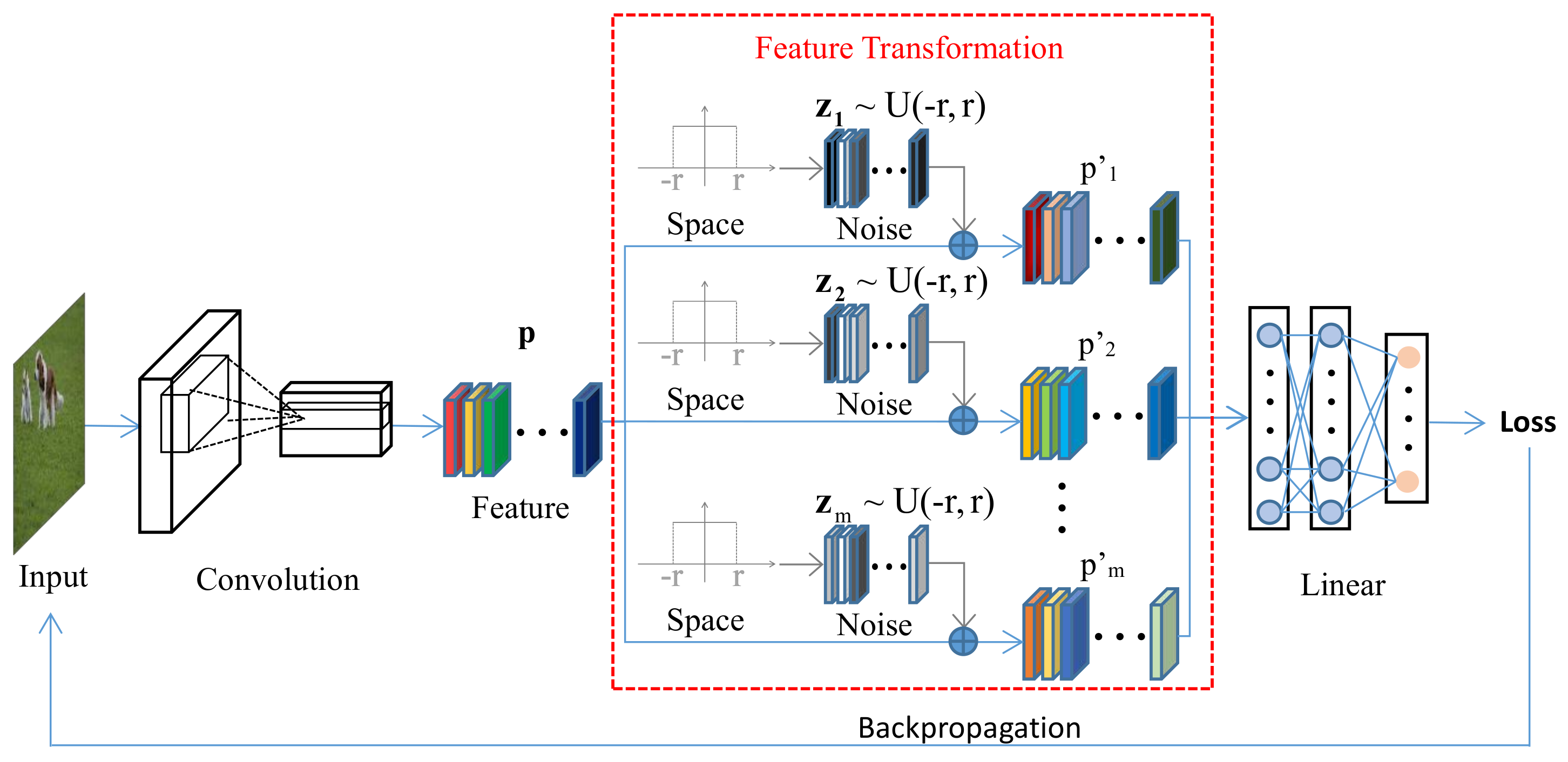
  • This work proposes a novel feature transformation-based method (FTM) for enhancing the transferability of adversarial examples.
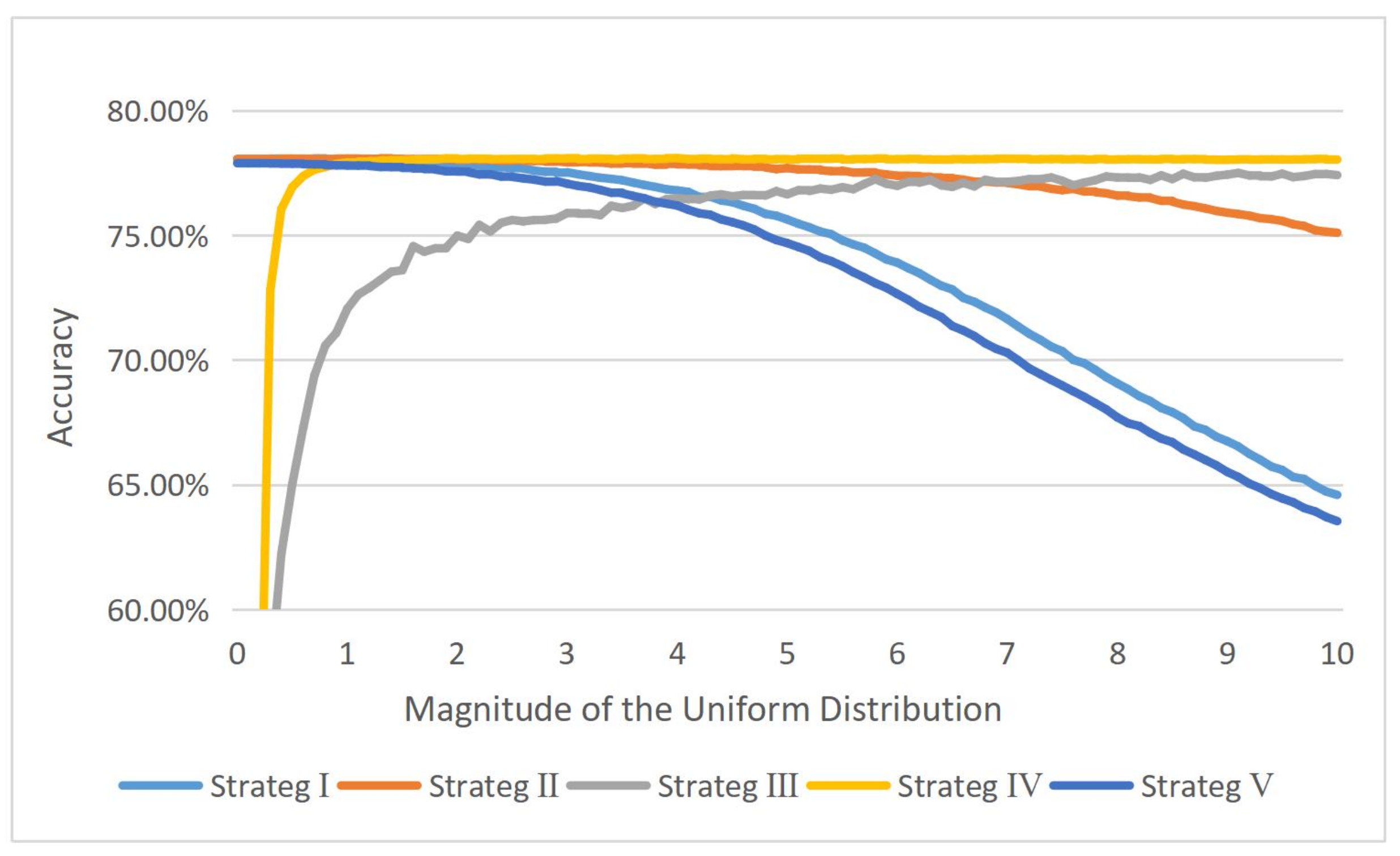
  • We propose several feature transformation strategies and comprehensively analyze the hyper-parameters of them.
  • The experimental results on two benchmark datasets show that FTM could effectively improve the attack success rate of the SOTA methods.
The structure of the paper is organized as follows. Section 2 introduces related work. Section 3 details the proposed FTM. Section 4 shows the experimental results. Section 5 gives a summary of this work.

2. Related Work

2.1. Adversarial Example and Transferability

It is firstly pointed out by Szegedy et al. [15] that DNNs are vulnerable to adversarial examples, which are generated by adding imperceptible noises to raw images.
Let x be a clean image, y = f ( x ; θ ) be the output label predicted by the model with parameters θ , and | | | | p denotes the p-norm. The adversarial example is an image x a d v whose output label f ( x a d v , θ ) f ( x , θ ) , and the L p norm of the adversarial perturbation x a d v x is smaller than a threshold ϵ as | | x a d v x | | ϵ . p = is used to limit the distortion. Many methods are proposed to improve the attack success rate (ASR) of adversarial examples. These methods can be divided into two branches: advanced gradient calculation and input transformations.

2.2. Advanced Gradient Calculation

This branch exploits better gradient calculation algorithms to enhance the performance of adversarial examples in both white-box settings and black-box settings.
Fast Gradient Sign Method (FGSM): Szegedy et al. [27] make the point that linear behavior in high-dimensional spaces is sufficient to cause adversarial examples. According to this point, they propose the FGSM, which generates an adversarial example x a d v by maximizing the loss function J ( x a d v , y ; θ ) with a one-step update:
x a d v = x + ϵ · s i g n ( x J ( x , y , θ ) )
where J ( x , y : θ ) denotes the loss function of classifier f ( x : θ ) , x J ( x , y , θ ) is the gradient of loss function with regard to x and s i g n ( · ) is the sign function to make the perturbation meet the L p norm bound.
Basic Iterative Method (BIM): Kurakin et al. [28] extend FGSM to an iterative version by iteratively applying gradient updates multiple times with a small step size α . BIM can be expressed as:
x t + 1 a d v = C l i p x ϵ { x t a d v + α · s i g n ( x J ( x , y , θ ) ) }
where x 0 = x and C i l p x ϵ ( · ) restricts generated adversarial examples to be within the ϵ -ball of x.
Momentum Iterative Fast Gradient Sign Method (MI-FGSM): To reduce the variation in update direction and avoid local minima, Dong et al. [34] introduce momentum into the BIM. The update procedure is formulated as follows:
g t + 1 = μ · g t + x J ( x , y , θ ) | | x J ( x , y , θ ) | | 1
x t + 1 a d v = C l i p x ϵ { x t a d v + α · s i g n ( g t + 1 ) }
where g t gathers the gradient of the first t iterations with a decay factor μ .
Nesterov Iterative Fast Gradient Sign Method (NI-FGSM): NI-FGSM [30] adopts Nesterov’s accelerated gradient to improve the transferability of MI-FGSM. This method replaces x t a d v in Equation (3) with x n e s t , while x n e s t can be formulated as follows:
x n e s t = x t a d v + α · μ · g t

2.3. Input Transformations

Various input transformation-based methods, such as DIM, TIM, SIM, and Admix, are proposed to generate transferable adversarial examples.
Diverse Input Method (DIM): Inspired by the facts that data augmentation is effective to prevent networks from overfitting, Xie et al. [31] apply random resizing and random padding to the inputs to improve the transferability of adversarial examples.
Translation-Invariant Method (TIM): Dong et al. [32] propose to replace the gradient on the original image with the average value of multiple translated images for the update. Inspired by the translation-invariant property, they approximate this process by convolving the gradient with a predefined kernel matrix to avoid introducing much more computations.
Scale-Invariant Method (SIM): Lin et al. [30] discover the scale-invariant property of deep learning models and introduce the definition of loss-preserving transformation and model augmentation. Accordingly, they present SIM that calculates the average gradient on the scaled copies of the original image for the update.
Admix Attack Method (Admix): Admix is proposed by [33] to enhance the transferability of the adversarial examples. It integrates gradient information of different categories of images for the update. Specifically, Admix randomly selects a number of different categories of images and then admix the sampled image with a minor weight to the original input image. It calculates the gradient on the mixed image for update.

2.4. Adversarial Defense

In addition to adversarial attacks, many works on adversarial defense have been proposed to improve the robustness of the classifiers. The current defense methods can be divided into two categories.
One category aims to improve the robustness of the classifier itself, such as adversarial training [27,35]. It adds adversarial examples to the training set during the training of the model, making it immune to the adversarial examples. This is a popular and effective defense method and has many great following works [36,37]. However, its effectiveness is largely limited by the method of generation of the added adversarial examples.
Another category of defense methods reduces the impact of adversarial perturbations by modifying the input images, such as adding noises and compressing the images [38,39]. Xie et al. [40] propose to perform randomized resizing and padding to inputs at inference time, which is the top-1 defense solution in the NIPS competition. Nips-r3 fuse multiple adversarial trained models and perform several input transformations at inference time. These methods require no additional training computational overhead and are effective against various attack approaches.

3. Our Approach

A DNN model could be formulated as f ( x ) = lin ( con ( x ) ) , where con ( · ) and lin ( · ) denote the convolutional part and the fully connected part, respectively. p = con ( x ) denotes the feature extracted by the convolutional part.
To obtain an ensemble of models that extract different features, we propose the feature transformation denoted as FT ( · ) . Through introducing feature transformation, we can obtain a new model f ( x ) = lin ( p ) = lin ( FT ( con ( x ) ) ) extracting different features from the original model during every iteration. FTM optimizes the adversarial perturbations over several different transformed features:
arg min x a d v 1 m i = 0 m J ( lin ( FT i ( con ( x a d v ) ) ) , y t r u e ) ,
s . t . , x a d v x ϵ ,
where m denotes the number of iterations and FT ( · ) denotes the feature transformation. Thus, FTM is an implicit ensemble attack that simultaneously attacks m models. The illustration of the FTM is shown in Figure 1.
In this paper, we consider five strategies of feature transformation as follows:
Strategy I: Fixed threshold random noise: Add a random vector z sampled from the uniform distribution U ( r , r ) :
FT ( p ) = p + z
Strategy II: Mean-based threshold random noise: z is a random vector sampled from the uniform distribution U ( r , r ) and p ¯ is the mean value of feature p . Adding p ¯ · z to feature p:
FT ( p ) = p + p ¯ · z
Strategy III: Feature overall scaled: Multiply the features p by a random number k sampled from the uniform distribution U ( r , r ) :
FT ( p ) = k · p
Strategy IV: Each value of feature scaled separately: Multiply feature p by a random vector z sampled from the uniform distribution U ( r , r ) :
FT ( p ) = z · p
Strategy V: Offset mean random noise: Add a random vector z sampled from the uniform distribution U ( r + s , r + s ) to feature p :
FT ( p ) = p + z
The feature transformation should also be an accuracy-preserving transformation. We define the accuracy-preserving feature transformation as follows:
Definition 1
(Acc-preserving Feature Transformation). Given a test set X and a classifier f ( x ) = lin ( con ( x ) ) , A c c ( lin ( con ( x ) ) , X ) denotes the accuracy of model f ( x ) on data set X. If there exists an feature transformation FT ( · ) that satisfies A c c ( lin ( con ( x ) ) , X ) A c c ( lin ( FT ( con ( x ) ) ) , X ) , we say FT ( · ) is an accuracy-preserving feature transformation.
We experimentally study the acc-preserving feature transformation strategies in Section 4.1.2. We determine the magnitude r of uniform distribution to ensure that our feature transformations are accuracy-preserving transformations. The algorithm of the FTM attack is summarized in Algorithm 1.
Algorithm 1 Algorithm of FTM.
Input: Original image x, true label y t r u e , a classifier f = lin ( con ( x ) ) , loss function J, feature transformation FT ( · )
Hyper-parameters: Perturbation size ϵ , maximum iterations T, number of iterations of feature transformation m
Output: Adversarial example x a d v
1: perturbation size in each iteration: α = ϵ / T
2: while  0 t < T 1 .
3: if  k = 0 .
4: x 0 = x .
5: end if
6: g = 0
7: while  0 i < m 1
8: feature: p = con ( x )
9: transformed feature: p = FT ( p )
10: Get the gradients by x J ( lin ( p ) , y t r u e )
11: Update g = g + x J ( lin ( p ) , y t r u e )
12: end while
13: Get average gradients as g ¯ = 1 m · g
14: Update x i + 1 a d v = Clip x ϵ { x i a d v + α · sign ( g ¯ ) }
15: end while
16: return x a d v = x T a d v

4. Experimental Results

4.1. Experiment on ImageNet

4.1.1. Experimental Setup

Dataset. We perform experiments on ImageNet, which is the most common and challenging image classification dataset. 1000 images from the ImageNet [41] are selected as our test set. The 1000 benign images belong to 1000 different categories and can be correctly classified by the tested models.
Networks. This work selects four mainstream models, including Inception_v3 (Inc_v3) [42], Inception_v4 (Inc_v4), Inception-Resnet_v2 (IncRes_v2) [43], and Xception(Xcep) [44].
Attack setting. We follow the setting in Lin et al. [30] with the maximum perturbation as ϵ = 16 , number of iteration T = 16 , and step size α = 1.6 , which is a difficult and challenging attack setting. We adopt the decay factor μ = 1.0 for MI-FGSM. The transformation probability is set to 0.5 for DIM. The number of scale copies is set to m = 5 for SIM. We set m 1 = 5 , and randomly sample m 2 = 3 images with η = 0.2 for Admix. The hyper-parameter settings of these attack methods are all consistent with the original papers.

4.1.2. Accuracy-Preserving Transformation

To investigate accuracy-preserving transformations, we test the accuracy of the models integrated with the five strategies on the ImageNet dataset. We keep the magnitude r of uniform distribution in the range of [ 0 , 10 ] .
The magnitude of uniform distribution is an important hyper-parameter of FTM. A larger magnitude will increase the diversity of the implicit ensemble models and thus improve the transferability of the adversarial examples. However, too large a magnitude will make the model invalid and thus lose the ability to guide the generation of AE. As shown in Figure 2, the accuracy curves are smooth and stable for strategies I, II, and V when the magnitude is in the range of [ 0 , 4 ] . They drop significantly after the magnitude exceeds 4. Moreover, the accuracies for strategy III and IV are extremely low when the magnitude is close to 0. They turn to remain stable after the magnitude exceeds 4. It can be seen that the feature transformation strategy with scaled operation is more sensitive to small magnitude, e.g., strategies III and IV. The feature transformation strategy of adding noise is more sensitive to a large magnitude, e.g., strategies I, II, and V. Based on the experimental results, the magnitude of uniform distribution is set to 4 in the following experiment to ensure that the feature transformations are accuracy-preserving transformations.

4.1.3. Feature Transformation Strategies

In this section, we show the experimental results of the proposed FTM with five feature transformation strategies. We set m = 1 and generate adversarial examples on the Inc_v3 by FT-FGSM, FT-MI-FGSM, and FT-SIM. The ASRs against the other three black-box models are presented in Table 1.
When combined with FT-FGSM, Strategy III achieves the best overall attack performance, reaching 35.9 % and 37.5 % when attacking IncRes_v2 and Xcep, respectively. When attacking with FT-MI-FGSM, Strategy V attains the best overall attack performance, reaching 57 % and 53.3 % when attacking Inv_v4 and IncRes_v2, respectively. When FT-SIM is used to attack IncRes_v2 and Xcep, Strategy III achieves the ASRs of 35.9 % and 37.5 % , which outperforms the other strategies. It can be seen that the overall performance of Strategy III is better and it performs better in the experiments combined with SIM, which is an input transformation-based method. Thus, we adopt Strategy III in the following experiments.

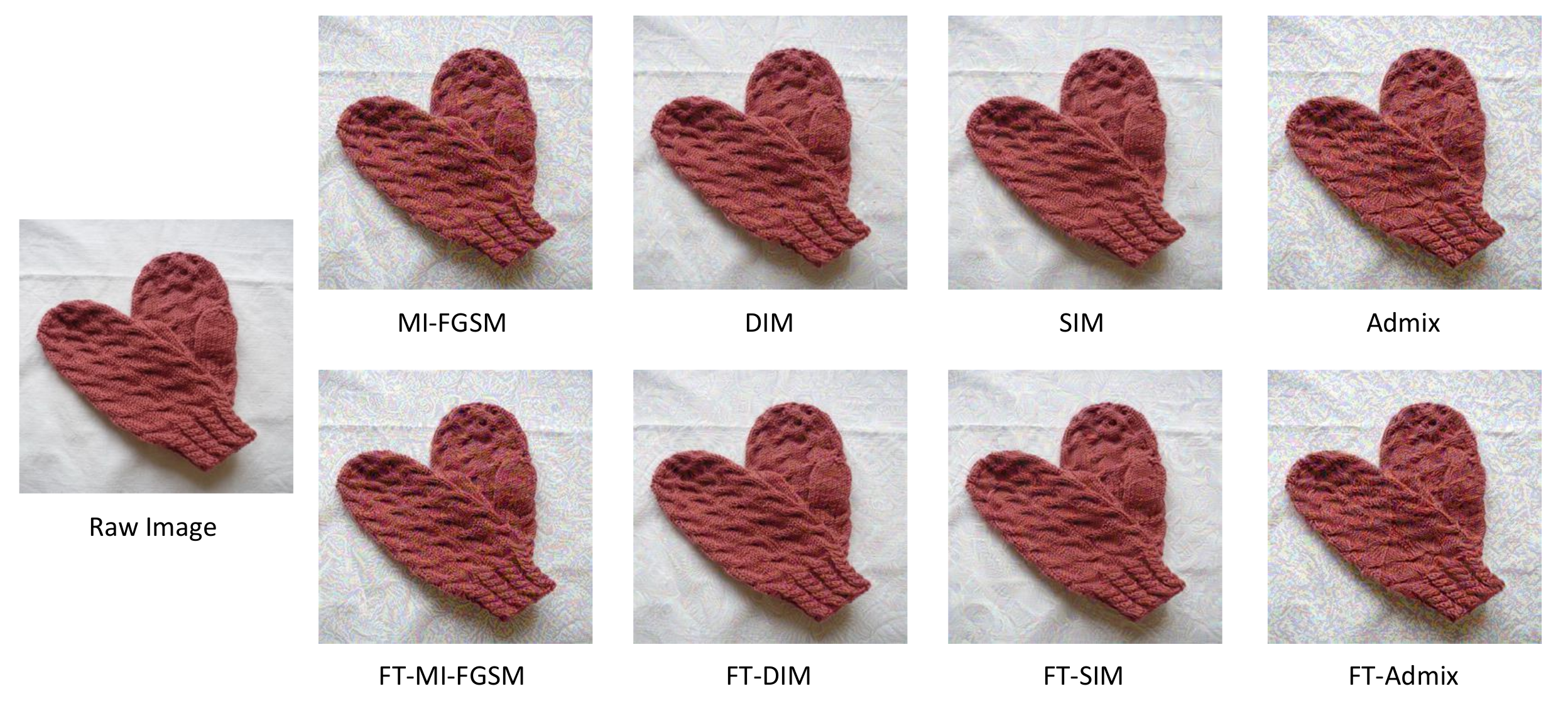
4.1.4. Attack with Input Transformations

We test the ASRs of MI-FGSM, SIM, DIM, and Admix, respectively. Then we combine these methods with FTM as FT-MI-FGSM, FT-SIM, FT-DIM, and FT-Admix. Some adversarial examples are shown in Figure 3. We adopt Strategy III, set m = 1 , set the magnitude of uniform distribution r = 4 , and then use the generated adversarial examples to attack the four models. We compare the black-box ASRs of FT-MI-FGSM, FT-SIM, FT-DIM, and FT-Admix with MI-FGSM, SIM, DIM, and Admix in Table 2, Table 3, Table 4 and Table 5. In the tables, the first columns are the local models, and the first rows are the target models. The values in the tables are the attack success rates (ASRs) on the target models using the adversarial examples generated from the local models. The higher ASRs are bolded.
When combined with MI-FGSM, the ASRs is increased by up to 9.4%, from 55% to 64.4% when attacking Xcep with Inc_v4. When FT-SIM is used to attack IncV3 with IncRes_v2, the ASR is improved from 62.6 % to 75.1 % , which outperforms the SIM by 12.5 % . The adversarial examples generated by FT-DIM achieved about 55 % ASR against all models. When FT-Admix is used to attack IncV3 with Xecp, the ASR reaches 72.2 % .
According to the reported experimental results, it can be observed that FTM could improve the ASRs of adversarial examples generated by the SOTA black-box attack methods. It is confirmed that feature transformation can improve the transferability and robustness of adversarial examples.

4.1.5. Attack against Defense Method

In this section, we quantify the effectiveness of FTM against several defense methods, including random resizing and padding (RandP) [40], JPEG compression (JPEG) [39], randomized smoothing (RS) [38], and the rank-3 submission in the NIPS-2017 (NIPS-r3). RandP is the top-1 submission in the NIPS competition, which mitigates the effect of adversarial perturbations by randomized resizing and padding. JPEG is a defensive compression framework, which could rectify adversarial examples without reducing classification accuracy on benign data. RS constructs a “smoothed” classifier from an arbitrary base classifier, which is more adversarially robust. NIPS-r3 fuses multiple adversarial trained models and performs several input transformation at inference time.
We choose SIM as the comparison method and generate adversarial examples with Inc_v3. The average ASRs on Inc_v4, IncRes_v2, and Xcep are shown in Table 6. The ASRs are improved by a large margin of 9.5% on average. It validates that the adversarial examples generated by FTM are more robust to fool models with defense mechanisms.

4.1.6. Parameter Analysis

In this section, we perform additional analysis for the difference among different numbers of iterations m. The adversarial examples are generated by FT-DIM on Inc_v3. The number of iterations of feature transformation ranges from 1 to 9.
As shown in Figure 4, the average black-box ASR increases from 59.2 % for 1 iteration to 62.7 % for 3 iterations. As the number of iterations increases to 9, the success rate of the attack increases to 65.3 % . It validates that the ASR of FTM increases as the number of iterations of feature transformation increases. The sensitivity of the attack success rate gradually decreases as the number of iterations increases. Since a higher number of iterations results in a larger computational overhead, the trade-off between effectiveness and overhead needs to be made according to the specific scenario.

4.2. Experiment on Cifar10

Cifar10

To further demonstrate the effectiveness of our approach, we also conducted experiments on the Cifar10 [45] dataset. Cifar10 has 60,000 color images with 32 × 32 pixels and is divided into 10 categories. We select 1000 images belonging to the 10 categories from the test set, which are correctly classified by all the experimental models. We compare the effects of the FTM with the MI-FGSM, SIM and Admix using the ResNet [46] family of models. The maximum perturbation ϵ = 4 , number of attack iterations T = 4 , and the step size α = 1 .
The experimental results for FT-MI-FGSM, FT-SIM, and FT-Admix are shown in Table 7, Table 8 and Table 9. The first columns are the local models and the first rows are the target models. It can be seen that our method improves the ASRs across all experiments. FT-MI-FGSM achieves 83.8 % ASR, when attacking Res152 with Res50. FT-SIM improves the ASR of SIM from 66.6 % to 73.9 % , when attacking Res101 with Res152. FT-Admix boosts the ASR of Admix attack from 43.1 % to 55.1 % , when attacking Res101 with Res152.
The experimental results on Cifar10 validate that FTM is effective not only on large image dataset, but also on small image dataset. Moreover, FTM can significantly improve the transferability and robustness of the adversarial examples generated by the SOTA black-box attack methods.

5. Conclusions

We propose a novel feature transformation-based method (FTM), which effectively improves the transferability of adversarial examples. Five feature transformation strategies are proposed and the hyper-parameters of them are comprehensively analyzed. The experimental results on two benchmark datasets show that FTM can improve the transferability of the adversarial example significantly. It improves the ASRs of the SOTA methods by up to 12.5% on ImageNet. Our method can be combined with not only any gradient-based attack methods but also any neural networks that can extract features. However, the tuning of hyper-parameters is difficult, because different models and feature transformation strategies require a large number of experiments to choose the magnitude of uniform distribution. In the future, we will explore more feature transformation strategies to improve the transferability of adversarial examples while reducing the difficulty of tuning hyper-parameters.

Author Contributions

Conceptualization, H.-Q.X. and C.H.; methodology, H.-Q.X., C.H. and H.-F.Y.; software, H.-Q.X.; data curation, H.-Q.X.; resources, C.H.; writing—original draft preparation, H.-Q.X., C.H. and H.-F.Y.; project administration, C.H.; funding acquisition, C.H. All authors have read and agreed to the published version of the manuscript.

Funding

This research was funded in part by the National Natural Science Foundation of China (Grant No. 62006097), in part by the Natural Science Foundation of Jiangsu Province (Grant No. BK20200593), in part by the China Postdoctoral Science Foundation (Grant No. 2021M701456), and in part by the Fundamental Research Funds for the Central Universities (Grant No. JUSRP121074).

Institutional Review Board Statement

Not applicable.

Informed Consent Statement

Not applicable.

Data Availability Statement

The ImageNet and Cifar10 datasets were analyzed in this study. The ImageNet dataset can be found at https://image-net.org/ (accessed on 10 July 2022). Cifar10 dataset can be found at https://www.cs.toronto.edu/~kriz/cifar.html (accessed on 10 July 2022).

Conflicts of Interest

The authors declare no conflict of interest.

References

  1. Gou, J.; Yuan, X.; Du, L.; Xia, S.; Yi, Z. Hierarchical Graph Augmented Deep Collaborative Dictionary Learning for Classification. IEEE Trans. Intell. Transp. Syst. 2022. [Google Scholar] [CrossRef]
  2. Gou, J.; Sun, L.; Du, L.; Ma, H.; Xiong, T.; Ou, W.; Zhan, Y. A representation coefficient-based k-nearest centroid neighbor classifier. Expert Syst. Appl. 2022, 194, 116529. [Google Scholar] [CrossRef]
  3. Gou, J.; He, X.; Lu, J.; Ma, H.; Ou, W.; Yuan, Y. A class-specific mean vector-based weighted competitive and collaborative representation method for classification. Neural Netw. 2022, 150, 12–27. [Google Scholar] [CrossRef] [PubMed]
  4. Koo, J.H.; Cho, S.W.; Baek, N.R.; Lee, Y.W.; Park, K.R. A Survey on Face and Body Based Human Recognition Robust to Image Blurring and Low Illumination. Mathematics 2022, 10, 1522. [Google Scholar] [CrossRef]
  5. Wang, T.; Ji, Z.; Yang, J.; Sun, Q.; Fu, P. Global Manifold Learning for Interactive Image Segmentation. IEEE Trans. Multimed. 2021, 23, 3239–3249. [Google Scholar] [CrossRef]
  6. Cheng, C.; Wu, X.J.; Xu, T.; Chen, G. UNIFusion: A Lightweight Unified Image Fusion Network. IEEE Trans. Instrum. Meas. 2021, 70, 1–14. [Google Scholar] [CrossRef]
  7. Liu, Q.; Fan, J.; Song, H.; Chen, W.; Zhang, K. Visual Tracking via Nonlocal Similarity Learning. IEEE Trans. Circuits Syst. Video Technol. 2018, 28, 2826–2835. [Google Scholar] [CrossRef]
  8. Zhu, X.F.; Wu, X.J.; Xu, T.; Feng, Z.H.; Kittler, J. Complementary Discriminative Correlation Filters Based on Collaborative Representation for Visual Object Tracking. IEEE Trans. Circuits Syst. Video Technol. 2021, 31, 557–568. [Google Scholar] [CrossRef]
  9. Ma, C.; Rao, Y.; Lu, J.; Zhou, J. Structure-Preserving Image Super-Resolution. IEEE Trans. Pattern Anal. Mach. Intell. 2021. [Google Scholar] [CrossRef]
  10. Gou, J.; Yu, B.; Maybank, S.J.; Tao, D. Knowledge distillation: A survey. Int. J. Comput. Vis. 2021, 129, 1789–1819. [Google Scholar] [CrossRef]
  11. Su, Y.; Zhang, Y.; Lu, T.; Yang, J.; Kong, H. Vanishing Point Constrained Lane Detection With a Stereo Camera. IEEE Trans. Intell. Transp. Syst. 2018, 19, 2739–2744. [Google Scholar] [CrossRef]
  12. Chen, Z.; Wu, X.J.; Yin, H.F.; Kittler, J. Robust Low-Rank Recovery with a Distance-Measure Structure for Face Recognition. In Proceedings of the PRICAI 2018: Trends in Artificial Intelligence, Nanjing, China, 28–31 August 2018; Geng, X., Kang, B.H., Eds.; Springer International Publishing: Cham, Switzerland, 2018; pp. 464–472. [Google Scholar]
  13. Kortli, Y.; Jridi, M.; Al Falou, A.; Atri, M. Face Recognition Systems: A Survey. Sensors 2020, 20, 342. [Google Scholar] [CrossRef]
  14. Adjabi, I.; Ouahabi, A.; Benzaoui, A.; Taleb-Ahmed, A. Past, Present, and Future of Face Recognition: A Review. Electronics 2020, 9, 1188. [Google Scholar] [CrossRef]
  15. Szegedy, C.; Zaremba, W.; Sutskever, I.; Bruna, J.; Erhan, D.; Goodfellow, I.; Fergus, R. Intriguing properties of neural networks. arXiv 2013, arXiv:1312.6199. [Google Scholar]
  16. Li, J.; Ji, R.; Liu, H.; Hong, X.; Gao, Y.; Tian, Q. Universal Perturbation Attack Against Image Retrieval. In Proceedings of the 2019 IEEE/CVF International Conference on Computer Vision (ICCV), Seoul, Korea, 27–28 October 2019; pp. 4898–4907. [Google Scholar] [CrossRef]
  17. Liu, H.; Ji, R.; Li, J.; Zhang, B.; Gao, Y.; Wu, Y.; Huang, F. Universal Adversarial Perturbation via Prior Driven Uncertainty Approximation. In Proceedings of the 2019 IEEE/CVF International Conference on Computer Vision (ICCV), Seoul, Korea, 27–28 October 2019; pp. 2941–2949. [Google Scholar] [CrossRef]
  18. Li, H.; Zhou, S.; Yuan, W.; Li, J.; Leung, H. Adversarial-Example Attacks Toward Android Malware Detection System. IEEE Syst. J. 2020, 14, 653–656. [Google Scholar] [CrossRef]
  19. Kwon, H.; Kim, Y.; Yoon, H.; Choi, D. Fooling a Neural Network in Military Environments: Random Untargeted Adversarial Example. In Proceedings of the MILCOM 2018—2018 IEEE Military Communications Conference (MILCOM), Los Angeles, CA, USA, 29–31 October 2018; pp. 456–461. [Google Scholar] [CrossRef]
  20. Zhu, Z.A.; Lu, Y.Z.; Chiang, C.K. Generating Adversarial Examples By Makeup Attacks on Face Recognition. In Proceedings of the 2019 IEEE International Conference on Image Processing (ICIP), Taipei, Taiwan, 22–25 September 2019; pp. 2516–2520. [Google Scholar] [CrossRef]
  21. Wang, K.; Li, F.; Chen, C.M.; Hassan, M.M.; Long, J.; Kumar, N. Interpreting Adversarial Examples and Robustness for Deep Learning-Based Auto-Driving Systems. IEEE Trans. Intell. Transp. Syst. 2021. [CrossRef]
  22. Rana, K.; Madaan, R. Evaluating Effectiveness of Adversarial Examples on State of Art License Plate Recognition Models. In Proceedings of the 2020 IEEE International Conference on Intelligence and Security Informatics (ISI), Arlington, VA, USA, 9–10 November 2020; pp. 1–3. [Google Scholar] [CrossRef]
  23. Hu, C.; Wu, X.J.; Li, Z.Y. Generating adversarial examples with elastic-net regularized boundary equilibrium generative adversarial network. Pattern Recognit. Lett. 2020, 140, 281–287. [Google Scholar] [CrossRef]
  24. Li, Z.; Feng, C.; Wu, M.; Yu, H.; Zheng, J.; Zhu, F. Adversarial robustness via attention transfer. Pattern Recognit. Lett. 2021, 146, 172–178. [Google Scholar] [CrossRef]
  25. Agarwal, A.; Vatsa, M.; Singh, R.; Ratha, N. Cognitive data augmentation for adversarial defense via pixel masking. Pattern Recognit. Lett. 2021, 146, 244–251. [Google Scholar] [CrossRef]
  26. Massoli, F.V.; Falchi, F.; Amato, G. Cross-resolution face recognition adversarial attacks. Pattern Recognit. Lett. 2020, 140, 222–229. [Google Scholar] [CrossRef]
  27. Goodfellow, I.J.; Shlens, J.; Szegedy, C. Explaining and Harnessing Adversarial Examples. arXiv 2014, arXiv:1412.6572. [Google Scholar]
  28. Kurakin, A.; Goodfellow, I.; Bengio, S. Adversarial examples in the physical world. In Proceedings of the International Conference on Learning Representations Workshop, Toulon, France, 24–26 April 2017; pp. 1–14. [Google Scholar] [CrossRef]
  29. Liu, Y.; Chen, X.; Liu, C.; Song, D. Delving into transferable adversarial examples and black-box attacks. In Proceedings of the International Conference on Learning Representations, Toulon, France, 24–26 April 2017; pp. 1–24. [Google Scholar]
  30. Lin, J.; Song, C.; He, K.; Wang, L.; Hopcroft, J.E. Nesterov Accelerated Gradient and Scale Invariance for Adversarial Attacks. In Proceedings of the International Conference on Learning Representations, Addis Ababa, Ethiopia, 26–30 April 2020; pp. 1–12. [Google Scholar]
  31. Xie, C.; Zhang, Z.; Zhou, Y.; Bai, S.; Wang, J.; Ren, Z.; Yuille, A.L. Improving Transferability of Adversarial Examples With Input Diversity. In Proceedings of the IEEE/CVF Conference on Computer Vision and Pattern Recognition (CVPR), Long Beach, CA, USA, 15–20 June 2019; pp. 2725–2734. [Google Scholar] [CrossRef]
  32. Dong, Y.; Pang, T.; Su, H.; Zhu, J. Evading Defenses to Transferable Adversarial Examples by Translation-Invariant Attacks. In Proceedings of the IEEE/CVF Conference on Computer Vision and Pattern Recognition (CVPR), Long Beach, CA, USA, 15–20 June 2019; pp. 4312–4321. [Google Scholar]
  33. Wang, X.; He, X.; Wang, J.; He, K. Admix: Enhancing the Transferability of Adversarial Attacks. In Proceedings of the IEEE/CVF International Conference on Computer Vision (ICCV), Montreal, BC, Canada, 11–17 October 2021; pp. 16158–16167. [Google Scholar]
  34. Dong, Y.; Liao, F.; Pang, T.; Su, H.; Zhu, J.; Hu, X.; Li, J. Boosting Adversarial Attacks with Momentum. In Proceedings of the 2018 IEEE/CVF Conference on Computer Vision and Pattern Recognition, Salt Lake City, UT, USA, 18–22 June 2018; pp. 9185–9193. [Google Scholar] [CrossRef]
  35. Kurakin, A.; Goodfellow, I.; Bengio, S. Adversarial Machine Learning at Scale. In Proceedings of the International Conference on Learning Representations, Toulon, France, 24–26 April 2017; pp. 1–17. [Google Scholar]
  36. Madry, A.; Makelov, A.; Schmidt, L.; Tsipras, D.; Vladu, A. Towards Deep Learning Models Resistant to Adversarial Attacks. In Proceedings of the International Conference on Learning Representations, Vancouver, BC, Canada, 30 April–3 May 2018; pp. 1–28. [Google Scholar]
  37. Tramèr, F.; Kurakin, A.; Papernot, N.; Goodfellow, I.; Boneh, D.; Mcdaniel, P. Ensemble Adversarial Training: Attacks and Defenses. In Proceedings of the International Conference on Learning Representations, Vancouver, BC, Canada, 30 April–3 May 2018; pp. 1–22. [Google Scholar]
  38. Cohen, J.M.; Rosenfeld, E.; Kolter, J.Z. Certified Adversarial Robustness via Randomized Smoothing. In Proceedings of the International Conference on Machine Learning, Long Beach, CA, USA, 9–15 June 2019; pp. 1–36. [Google Scholar]
  39. Guo, C.; Rana, M.; Cisse, M.; van der Maaten, L. Countering Adversarial Images using Input Transformations. In Proceedings of the International Conference on Learning Representations, Vancouver, BC, Canada, 30 April–3 May 2018; pp. 1–12. [Google Scholar]
  40. Xie, C.; Wang, J.; Zhang, Z.; Ren, Z.; Yuille, A. Mitigating Adversarial Effects Through Randomization. In Proceedings of the International Conference on Learning Representations, Toulon, France, 24–26 April 2017; pp. 1–16. [Google Scholar]
  41. Russakovsky, O.; Deng, J.; Su, H.; Krause, J.; Satheesh, S.; Ma, S.; Huang, Z.; Karpathy, A.; Khosla, A.; Bernstein, M.; et al. Imagenet large scale visual recognition challenge. Int. J. Comput. Vis. 2015, 115, 211–252. [Google Scholar] [CrossRef]
  42. Szegedy, C.; Vanhoucke, V.; Ioffe, S.; Shlens, J.; Wojna, Z. Rethinking the Inception Architecture for Computer Vision. In Proceedings of the IEEE Conference on Computer Vision and Pattern Recognition (CVPR), Los Alamitos, CA, USA, 27–30 June 2016; pp. 2818–2826. [Google Scholar] [CrossRef]
  43. Szegedy, C.; Ioffe, S.; Vanhoucke, V.; Alemi, A.A. Inception-v4, Inception-ResNet and the Impact of Residual Connections on Learning. In Proceedings of the Thirty-First AAAI Conference on Artificial Intelligence, San Francisco, CA, USA, 4–9 February 2017; pp. 4278–4284. [Google Scholar]
  44. Chollet, F. Xception: Deep Learning with Depthwise Separable Convolutions. In Proceedings of the 2017 IEEE Conference on Computer Vision and Pattern Recognition (CVPR), Honolulu, HI, USA, 21–27 July 2017; pp. 1800–1807. [Google Scholar] [CrossRef]
  45. Krizhevsky, A. Learning Multiple Layers of Features from Tiny Images; University of Toronto: Toronto, ON, USA, 2009; pp. 1–60. [Google Scholar]
  46. He, K.; Zhang, X.; Ren, S.; Sun, J. Deep residual learning for image recognition. In Proceedings of the IEEE Conference on Computer Vision and Pattern Recognition, Las Vegas, NV, USA, 27–30 June 2016; pp. 770–778. [Google Scholar]
Figure 1. Illustration of the proposed FTM. The feature transformation shown in the illustration is the Strategy I. The random noise vectors z i sampled from the uniform distribution are added to the feature p . The average loss of the transformed features is calculated to update the input image.
Mathematics 10 02976 g001
Figure 2. The average classification accuracy of Inc_v3, Inc_v4, IncRes_v2, and Xcep integrated with five different feature transformation strategies on ImageNet. The horizontal coordinate is the magnitude of uniform distribution and the vertical coordinate is the accuracy of the model.
Mathematics 10 02976 g002
Figure 3. Adversarial examples generated by MI-FGSM, DIM, SIM, Admix, the proposed FT-MI-FGSM, FT-DIM, FT-SIM, and FT-Admix on the Inc_v3.
Mathematics 10 02976 g003
Figure 4. The black-box ASRs of FT-DIM attack with different number of iterations on ImageNet. The adversarial examples are generated on Inc_v3 and the ASRs are the average ASRs on Inc_v4, IncRes_v2, and Xcep.
Mathematics 10 02976 g004
Table 1. The black-box ASRs (%) of FT-FGSM, FT-MI-FGSM, and FT-SIM with five strategies on ImageNet. The adversarial examples are generated on Inc_v3. The highest ASRs are shown in bold.
MethodStrategyInc_v3Inc_v4IncRes_v2Xcep
I-36.133.535.3
II-37.333.735.1
FT-FGSMIII-37.035.937.5
IV-37.532.034.7
V-37.733.434.4
I-55.152.559.8
II-53.050.454.4
FT-MI-FGSMIII-54.951.657.8
IV-53.450.856.5
V-57.053.359.2
I-43.041.342.9
II-38.534.939.3
FT-SIMIII-42.942.644.0
IV-42.242.443.5
V-41.141.942.6
Table 2. The black-box ASRs of MI-FGSM and FT-MI-FGSM on ImageNet. The first column is the local model, and the first row is the target model. The values in the table are the ASRs (%) on the target models using the adversarial examples generated with the local models. The higher ASRs are shown in bold.
Local ModelAttack MethodInc_v3Inc_v4IncRes_v2Xcep
Inc_v3MI-FGSM-51.349.653.0
FT-MI-FGSM-54.951.657.8
Inc_v4MI-FGSM56.0-48.555.0
FT-MI-FGSM58.9-53.164.4
IncRes_v2MI-FGSM56.251.8-55.9
FT-MI-FGSM64.157.4-63.0
XcepMI-FGSM51.450.845.3-
FT-MI-FGSM54.455.048.7-
Table 3. The black-box ASRs of SIM and FT-SIM on ImageNet. The first column is the local model, and the first row is the target model. The values in the table are the ASRs (%) on the target models using the adversarial examples generated with the local models. The higher ASRs are shown in bold.
Local ModelAttack MethodInc_v3Inc_v4IncRes_v2Xcep
Inc_v3SIM-37.434.737.0
FT-SIM-42.942.644.0
Inc_v4SIM64.0-51.959.7
FT-SIM71.0-59.064.9
IncRes_v2SIM62.652.8-55.2
FT-SIM75.163.4-65.2
XcepSIM57.954.350.0-
FT-SIM63.458.953.0-
Table 4. The black-box ASRs of DIM and FT-DIM on ImageNet. The first column is the local model, and the first row is the target model. The values in the table are the ASRs (%) on the target models using the adversarial examples generated with the local models. The higher ASRs are shown in bold.
Local ModelAttack MethodInc_v3Inc_v4IncRes_v2Xcep
Inc_v3DIM-59.555.356.3
FT-DIM-61.858.360.4
Inc_v4DIM59.0-52.061.7
FT-DIM63.4-56.566.6
IncRes_v2DIM58.657.7-60.7
FT-DIM67.266.8-66.5
XcepDIM57.364.355.6-
FT-DIM61.869.158.2-
Table 5. The black-box ASRs of Admix and FT-Admix on ImageNet. The first column is the local model, and the first row is the target model. The values in the table are the ASRs (%) on the target models using the adversarial examples generated with the local models. The higher ASRs are shown in bold.
Local ModelAttack MethodInc_v3Inc_v4IncRes_v2Xcep
Inc_v3Admix-52.849.156.2
FT-Admix-57.354.460.0
Inc_v4Admix70.8-61.167.2
FT-Admix72.2-64.068.3
IncRes_v2Admix64.157.4-60.5
FT-Admix66.058.7-60.4
XcepAdmix70.464.360.0-
FT-Admix72.265.261.6-
Table 6. The black-box ASRs of SIM and FT-SIM on ImageNet against four defense methods. The adversarial examples are generated with Inc_v3. The values in the table are the average ASRs (%) on the Inc_v4, IncRes_v2, and Xcep. The higher ASRs are shown in bold.
Attack MethodRandPJPEGRSNips-r3
SIM30.332.725.231.6
FT-SIM38.541.037.839.5
Table 7. The black-box ASRs of MIM (MI-FGSM) and FT-MIM (FT-MI-FGSM) on Cifar10. The first column is the local model, and the first row is the target model. The values in the table are the ASRs (%) on the target models using the adversarial examples generated with the local models. The higher ASRs are shown in bold.
Local ModelAttack MethodRes18Res34Res50Res101Res152
Res18MIM-78.368.767.371.1
FT-MIM-78.869.270.573.4
Res34MIM78.7-70.069.572.3
FT-MIM79.8-72.971.274.1
Res50MIM76.576.8-80.282.5
FT-MIM77.878.1-82.483.8
Res101MIM71.471.776.9-80.5
FT-MIM74.273.279.3-82.6
Res152MIM75.273.476.881.0-
FT-MIM76.874.978.782.0-
Table 8. The black-box ASRs of SIM and FT-SIM on Cifar10. The first column is the local model, and the first row is the target model. The values in the table are the ASRs (%) on the target models using the adversarial examples generated with the local models. The higher ASRs are shown in bold.
Local ModelAttack MethodRes18Res34Res50Res101Res152
Res18SIM-73.060.159.562.3
FT-SIM-73.962.262.966.0
Res34SIM74.9-60.260.963.3
FT-SIM76.2-61.562.863.4
Res50SIM68.069.3-70.671.9
FT-SIM72.268.2-73.976.0
Res101SIM69.267.771.0-73.9
FT-SIM71.569.971.9-75.9
Res152SIM65.662.363.866.6-
FT-SIM69.567.970.473.9-
Table 9. The black-box ASRs of Admix and FT-Admix on Cifar10. The first column is the local model, and the first row is the target model. The values in the table are the ASRs (%) on the target models using the adversarial examples generated with the local models. The higher ASRs are shown in bold.
Local ModelAttack MethodRes18Res34Res50Res101Res152
Res18Admix-49.041.942.545.0
FT-Admix-56.447.350.451.9
Res34Admix52.5-42.746.546.0
FT-Admix58.5-47.550.150.4
Res50Admix48.643.9-44.947.4
FT-Admix56.150.7-53.954.4
Res101Admix48.244.644.6-49.3
FT-Admix54.050.550.8-57.7
Res152Admix45.340.639.543.1-
FT-Admix55.051.650.255.1-
Publisher’s Note: MDPI stays neutral with regard to jurisdictional claims in published maps and institutional affiliations.

