Pulse of the Nation: Observable Subjective Well-Being in Russia Inferred from Social Network Odnoklassniki

Abstract

Policymakers and researchers worldwide are interested in measuring the subjective well-being (SWB) of populations. In recent years, new approaches to measuring SWB have begun to appear, using digital traces as the main source of information, and show potential to overcome the shortcomings of traditional survey-based methods. In this paper, we propose the formal model for calculation of observable subjective well-being (OSWB) indicator based on posts from a social network, which utilizes demographic information and post-stratification techniques to make the data sample representative by selected characteristics of the general population. We applied the model on the data from Odnoklassniki, one of the largest social networks in Russia, and obtained an OSWB indicator representative of the population of Russia by age and gender. For sentiment analysis, we fine-tuned several language models on RuSentiment and achieved state-of-the-art results. The calculated OSWB indicator demonstrated moderate to strong Pearson’s ($r=0.733$, $p=0.007$, $n=12$) correlation and strong Spearman’s ($r_s=0.825$, $p=0.001$, $n=12$) correlation with a traditional survey-based Happiness Index reported by Russia Public Opinion Research Center, confirming the validity of the proposed approach. Additionally, we explored circadian (24 h) and circaseptan (7 day) patterns, and report several interesting findings for the population of Russia. Firstly, daily variations were clearly observed: the morning had the lowest level of happiness, and the late evening had the highest. Secondly, weekly patterns were clearly observed as well, with weekends being happier than weekdays. The lowest level of happiness occurs in the first three weekdays, and starting on Thursday, it rises and peaks during the weekend. Lastly, demographic groups showed different levels of happiness on a daily, weekly, and monthly basis, which confirms the importance of post-stratification by age group and gender in OSWB studies based on digital traces.

1. Introduction

Throughout history, philosophers have considered happiness to be the highest good and the ultimate motivation of human action [1]. Subjective well-being (SWB), also known as the scientific term for happiness and life satisfaction, is used to describe the level of well-being people experience according to their subjective evaluations of their lives [2]. Recently, practical interest in SWB has also been shown by government agencies, considering SWB indicators as one of the key guidelines for the development of the state instead of the currently utilized indicators, such as gross domestic product [3].

Individuals’ levels of SBW are influenced both by internal factors, such as personality [4] and outlook, and external factors, such as the society they live in or life events; thus, people’s SWB is subject to constant changes. Traditionally, SWB is measured through self-report surveys. Although these surveys are considered accurate and valid for measuring SWB [5], they also suffer from some considerable pitfalls. For example, self-reported answers may be exaggerated [6], various biases may affect the results (e.g., social desirability bias [7], question order bias [8], and demand characteristics [9]), momentary mood may influence the subjects’ responses to SWB questions [10], and people tend to recall past events that are consonant with their current affect [11]. Moreover, self-report surveys cannot provide constant updates of well-being to researchers and policymakers, and the cost of conducting them tends to be relatively high, thereby making it challenging for many countries to estimate well-being frequently [12,13,14]. In addition to the methodological and practical challenges of conducting self-report survey studies, there has been a recent decline in the level of trust in the results of such studies in several countries, particularly in Russia. According to the survey [15] conducted by Russia Public Opinion Research Center in 2019, the index of trust in sociological data has continued to decline among Russians over the past three years. The total level of credibility of the results of social research was 58% (this is the total share of respondents who agree that the polls really reflect the real opinion of citizens). At the same time, 37% of citizens are skeptical about the results of opinion polls. Every second respondent (53%) thinks that the poll results are fabricated in order to influence people, persuading them to behave in a certain way. According to the opinion poll [16] by the Public Opinion Foundation in 2020, every third Russian (36%) does not trust the data of opinion polls.

Over the past few decades, there has been much progress in the measurement of SWB [17]. In particular, researchers across disciplines have proposed several innovative digital data sources, also called digital traces, and methods that have the potential to overcome the limitations of traditional survey-based methods [14], including measuring individual and collective well-being [13]. According to Howison et al. [18], digital trace data are found (rather than produced for research), and event-based (rather than summary data), and longitudinal (since events occur over a period of time) data are both produced through and stored by an information system. One of the most commonly used types of digital traces in SWB studies is user-generated content from social networks [12,19]. The most important epistemological advantage of digital trace data is that they present observed (In general, this issue can be debatable for different types of digital traces. For example, in the case of posts from social networks, the source of these data is still the subject with their subjective assessments, which are influenced by many factors. In the framework of this study, we still perceive these data as observable, since the data were originally generated by the subjects not for research, but for personal purposes.) instead of self-reported behavior [20], which is also characterized by real-time observation with continuous follow-up.

Moreover, due to the presence of digital trace data spread over time, it provides researchers with the opportunity to conduct studies that are otherwise impossible or at least difficult to conduct using traditional approaches [14]. Although there is still considerable controversy surrounding the classification, so far, most psychology research [21] has conceptualized SWB as either an assessment of life satisfaction or dissatisfaction (evaluative well-being measures) or as a combination of experienced affect (experienced well-being measures). At the same time, there is also a degree of uncertainty around the terminology in studies measuring SWB based on digital traces because they cannot be unambiguously attributed to either evaluative or experienced measures. We propose to use the term observable subjective well-being (OSWB), which explicitly characterizes the data source as observed (not self-reported) and does not make any assumptions about the evaluative or experienced nature of the data (both can be presented in different proportions).

A growing body of literature [13,22,23] investigates different variations of OSWB indices calculated based on textual content from social media sites. For example, changes in the level of happiness and mood based on tweets were explored for the United States of America [24,25], the United Kingdom [26,27,28], China [29], Italy [30], the UAE [31], and Brazil [32]. However, one of the main challenges with existing studies is the lack of representative data—in terms of the data source, general population of internet users, or general population of the analyzed country. Although for many other languages, OSWB studies have already been conducted, the research of Russian-language content (e.g., [33,34,35]) remains quite limited and targets particular social networks, groups of users, or regions, but not the general population of Russia. For example, Panchenko [33] analyzed the Russian-language segment of Facebook by using a rule-based sentiment classification model with low classification quality. (Panchenko [33] used a dictionary based approach for sentiment analysis of Facebook posts, but tested it on the Books, Movies, and Cameras subsets of the ROMIP 2012 dataset [36]. The average accuracy for these 3 subsets was 32.16 and average $F_1$ was 26.06. At the same time, the classification metrics that the authors of the dataset were able to achieve when publishing it is higher [36].) He did not consider the demographics of the users, and did not measure the reliability of the proposed approach (although the last two items seem to be out of scope of Panchenko’s study). Shchekotin et al. [34] analyzed posts of 1350 of the most popular Vkontakte regional and urban communities, but they likewise did not consider any demographic characteristics and did not measure the reliability of the proposed approach. Kalabikhina et al. [35] explored the demographic temperature of 314 pro-natalist groups (with child-born reproductive attitudes) and 8 anti-natalist (with child-free reproductive attitudes) Vkontake groups. In general, all these studies were focused on the particular group of users or a sample of a social network audience, but they did not project the results with respect to the general population of Russia. Moreover, studies about Russian-language content suffer from a series of disadvantages, outlined in our recent review paper [37]. Furthermore, a recent poll [15] by the Russia Public Opinion Research Center (VCIOM) showed that the overwhelming majority (91%) of Russians are convinced that research of public opinion is necessary. The majority of Russians (78%) believe that public opinion polls help to determine the opinion of people about the situation in their place of residence so that the authorities can take into account the opinion of the people when solving painful problems. Moreover, according to another recent survey [38] by VCIOM, welfare and well-being were most often cited by respondents as the main goals of Russia in the 21st century. Measures of SWB are likely to play an increasingly important role in policy evaluation and decisions because not only do both policymakers and individuals value subjective outcomes, but such outcomes also appear to be affected by major policy interventions [17].

In this paper, we propose the formal model for calculation of the OSWB indicator based on posts from the chosen social network, which utilizes demographic information and post-stratification techniques to make the data sample representative by selected characteristics of the general population. We applied the model on the data from Odnoklassniki, one of the largest social networks in Russia, and obtained OSWB indicator representative of the population of Russia by age and gender. For sentiment analysis, we fine-tuned several language models on the RuSentiment dataset [39] and achieved state-of-the-art (SOTA) results of weighted $F_1=76.30$ (4.27 percentage points above existing SOTA) and macro $F_1=78.92$ (0.42 percentage points above existing SOTA). The calculated OSWB indicator demonstrated moderate to strong Pearson’s ($r=0.733$) correlation and strong Spearman’s ($r_s=0.825$) correlation with a traditional survey-based indicator reported by Russia Public Opinion Research Center (VCIOM) [40], confirming the acceptable level of validity of the proposed indicator. Considering that the typical reliability of SWB scales is in the range of 0.50 to 0.84 [21,41,42,43,44,45] (and even between 0.40 and 0.66 for single-items measures, such as VCIOM Happiness [42]) corrected for unreliability, the real correlation is practically close to unity. Thus, we assume that the obtained correlation can be interpreted not as moderate, but as one of the highest correlations that can be achieved in behavioral sciences. Additionally, we explored circadian (24 h) and circaseptan (7 day) patterns, and report several interesting findings for the population of Russia (see Section 5.1 and Section 5.2).

The rest of the article is organized as follows. Section 2 describes related work, including existing SWB and OSWB studies, sentiment analysis, and comparisons of text analysis methods and traditional survey methods in sociological research. Section 3 presents a model for the calculation of the OSWB indicator based on posts from the social network. Section 4 describes the data from Odnoklassniki used for real-life application of the proposed model and sentiment classification models. Section 5 highlights key results of the Odnoklassniki data analysis. Section 6 provides the discussion of the results of the study. Section 7 describes the key limitations of the study. In Section 8, conclusions are drawn, and the main contributions of the study are articulated.

2. Related Work

2.1. Happiness and the Economy

National financial measures, such as gross domestic product (GDP), are typically used to assess policy effectiveness. However, GDP has been criticized as a weak indicator of well-being and, therefore, a misleading measure of national success and tool for public policies [13,46,47,48]. In 2011, the UN General Assembly, at the 65th session on the initiative of Bhutan and with the support of more than 50 states, adopted Resolution A/RES/65/309 entitled “Happiness: Towards a Holistic Approach to Development”. Recognizing that GDP by nature was not designed to and reflect the happiness and well-being of individuals in a country, the UN general assembly invited member states to pursue the elaboration of additional measures that can better capture the importance of the pursuit of well-being and happiness in development with a view to guide their public policies.

According to Yashina [49], the level of material well-being is an essential but not the decisive factor in the happiness of the inhabitants of Russia. Measuring the SWB is not yet used at the state level in Russia as a criterion for assessing the success of the socio-economic development of the country, although this issue is being discussed [50]. (For example, the Chairman of the Federation Council of the Federal Assembly of the Russian Federation supported the proposal to measure the happiness index of Russians to assess government decisions [51].) At the same time, state bodies in a number of other countries have already been created to deal with problems of happiness—for instance, Gross National Happiness Center in Butan, Gross National Happiness Center in Thailand, Ministry of Higher Social Happiness in Venezuela, and World Happiness Council in the United Arab Emirates. Thus, the issue of regularly measuring the well-being of Russians at the state level is relevant, and measuring the SWB based on digital traces can become one of the tools due to the previously described advantages over classical survey approaches.

2.2. Subjective Well-Being

Well-being, happiness, and life satisfaction are an integral part of many cross-country comparative studies of the quality of life, which are carried out at the initiative of international organizations and governments [3]. Considering the subjective nature of happiness, researchers frequently measure it by self-report rating scales [13,19]. Despite some debate over the best way to conceptualize and measure the affective component of SWB, most researchers agree that the frequency of emotions, rather than their intensity, is the best indicator of the affective component [52]. In particular, there have been further studies confirming that it is the frequency of emotions that matter for measuring SWB, even in the absence of a psychometric survey, e.g., the emotional recall task is a mostly semantic/psycholinguistic task that has been shown to correlate strongly with PANAS indicators in English speakers [53]. Examples of self-reported surveys are the Gallup World Poll, the World Values Survey, the Eurobarometer, the European Quality of Life Surveys, and the British Household Panel Survey. Some of these organizations conduct surveys in many countries across the world, including Russia. (For example, according to Gallup World Pull survey [54], in 2021, the Index of Russians’ Happiness fell to a ten-year low: only 41% of Russians consider themselves happy, and about a quarter are unhappy.) A growing number of Russian research organizations are becoming involved in the collection of SWB data. In particular, Almakaeva and Gashenina [3] highlighted the following research organizations: Russia Public Opinion Research Center, Public Opinion Foundation, Levada Center, the Institute of Psychology of Russian Academy of Sciences, the Russia Longitudinal Monitoring Survey of HSE University, the Center for Sociological Research of Russian Presidential Academy of National Economy and Public Administration, and the Ronald F. Inglehart Laboratory for Comparative Social Research of HSE University. In comparison with international organizations, Russian organizations tend to focus more on researching well-being in Russia and in different aspects thereof. (For example, one of the most famous indices in Russia is the Happiness Index, calculated by VCIOM. According to VCIOM data for November 2021 [55], the majority of Russians (84%) consider themselves happy, whereas 14% do not. Most often, Russians consider themselves happy due to the health and life of their own and those of their loved ones (29%), due to the fact that they have a family (27%), have children (22%), have general satisfaction with life (21%), or a good job (12%)).

Due to the widespread interest from research and government organizations, many methodological materials (e.g., [43,56,57,58]) have been developed for measuring SWB through surveys. Although self-report surveys have been considered accurate and valid for measuring SWB [5], they also suffer from some considerable pitfalls. One of the main limitations of classical survey polls is reactivity: respondents and subjects almost always know that they are participating in the study, and this, in turn, can have an effect on the results of the study [14]. Self-reported answers may be exaggerated [6], numerous biases may affect the results (e.g., question order bias [8], demand characteristics [9], and social desirability bias [7]), momentary mood may influence subjects’ responses to SWB questions [10], and respondents tend to recall past events that are consonant with their current affect [11]. Additionally, a recognition-based checklist may fail to capture sufficient breadth and specificity of an individual’s recalled emotional experiences and may therefore miss emotions that frequently come to mind [53]. The relatively small sample size in the surveys limits the search for heterogeneous relationships and patterns between the studied concepts [14]. Moreover, self-report surveys cannot provide constant updates of well-being to researchers and policymakers, and they incur relatively high costs to be conducted, thereby making it challenging for many countries to estimate well-being frequently [12,13,14]. Given the formidable list of limitations, over the past few decades, there has been much progress in the measurement of SWB [17]. Researchers across disciplines have proposed several innovative digital data sources, also called digital traces, and methods that have the potential to overcome the limitations of traditional survey-based methods [14], including measuring individual and collective well-being [13].

2.3. Observable Subjective Well-Being

In recent years, there has been an increasing amount of literature on OSWB indices based on digital sources, especially using posts from social networks [12,13,19]. The key idea of these studies is to replace people with texts as the unit of analysis and apply natural language processing (NLP) techniques to quantify expressed sentiment. From the sentiment expression point of view, all existing approaches for OSWB indices calculation can be divided in two groups: word-level (e.g., [59]) and text-level (e.g., [24]) approaches. Word-level approaches analyze texts at the word level, calculate the number of emotionally charged words based on dictionaries of tonal vocabulary, and then calculate indices based on the data obtained. This type of approach has been widely criticized in the literature. For example, it has been shown by Wang et al. [60] that one of the most famous such indices, Facebook’s Gross National Happiness [59], is a valid measure for neither mood nor well-being. Moreover, from an etymological point of view, word-level approaches suffer from the fact that they miss part of the sentiments expressed in a different way than just in words. Emotions in the text can be represented both at the level of form and at the level of content, expressed implicitly and explicitly [61]. In the recent survey on sentiment analysis of texts in Russian [62], it was also mentioned that sentiment can be expressed explicitly using specialized sentiment words and implicitly using sentiment facts [63] or words with connotations [64]. Thus, word-level approaches cannot display the full picture because they ignore part of the emotions presented in the text by definition; therefore, recent studies more often focus on text-level approaches. In contrast with word-level approaches, text-level approaches analyse the entire text, attempting to capture all sentiment presented, and for each text return a sentiment class or a group of sentiment classes presented. Thus, we decided to focus only on the text-level approaches.

Extensive review of existing OSWB studies has been performed in recent articles [13,19,23], so we will not focus in detail on describing existing work and instead consider their challenges and limitations. Firstly, the lack of domain-specific training data and representative data for the analysis is a major challenge [23], including for the Russian language [37]. Secondly, very few studies (just over 1% according to [23]) use deep learning, which can help to achieve a higher quality sentiment classification in contrast with rule-based and traditional machine learning methods, as already demonstrated for the Russian language [65,66,67,68,69]. Thirdly, there are significant theoretical knowledge gaps regarding best practices and guidelines for calculating OSWB indices based on digital traces. For example, demographic information is rarely used (slightly less than 5% according to [23]), which may call into question the representativeness of the results obtained. In classical survey research, the sampling design is intended to accommodate different demographic groups in proportion to their distribution in the target population, so the results are representative of the target population. This is also the case for OSWB studies [24,25,26,27,28,29,30,31,32] mentioned earlier. In the context of digital traces, access to such information is usually difficult or impossible. According to the European Social Survey Sampling Guidelines [58], which are also used for measuring and reporting on Europeans’ well-being [70], individual-level variables (e.g., gender and age) tend to be more beneficial than regions or characteristics of small areas (e.g., local unemployment rate and population density). Thus, the presence of these demographic variables tends to be crucial for OSWB research to perform post-stratification and make results representative of the general population of the analyzed country. Lastly, there is still significant controversy about correspondence of digital traces to survey data [19,60,71,72,73]. More specifically, it is often asked whether social media content really represents the state of affairs in the offline world. According to a study by Dudina [74], claiming that a social media discussion shows only the reactions of social media users is tantamount to believing that the answers to the survey questions reflect only the opinions of the people who answered those questions, without the possibility of extrapolating the results to wider groups. This, in turn, is tantamount to rejecting the idea of representativity in the social sciences. Supporting a similar idea, Schober et al. [75] stated that traditional population coverage may not be required for social media analysis to effectively predict social phenomena to the extent that social media content distills or summarizes broader conversations that are also measured by surveys. Despite the disagreements between the existing points of view, it should be noted that the issue of validating the results obtained is extremely important. We believe that some of the existing methods of the social sciences can be used to determine the validity of the results obtained on the basis of electronic traces. Obviously, not all of them are suitable for working with digital traces due to nature of the data. For example, it remains an open question how to perform a face validity or test-retest reliability [43] checks given that OSWB researchers commonly lack additional information beyond the digital traces themselves and some information the users specified on their online profiles. However, we argue that a number of other checks outlined in the OECD Guidelines on Measuring SWB [43] can be used to check the results; for example, validity can be tested by comparing results with different measures.

As for the OSWB studies focused on Russian content, the literature remains quite limited and, as our previous survey [37] has shown, is one of the promising areas of research. For example, Panchenko [33] built several sentiment indicators for Russian-language Facebook. Shchekotin et al. [34] proposed a method for subjective assessment of well-being in Russian regions based on VKontakte data. Sivak and Smirnov [73] examined correlations between self-reports and digital trace proxies of depression, anxiety, mood, social integration, and sleep among high school students. Kalabikhina et al. [35] analyzed the demographic temperature (ratio of positive and negative comments) in certain sociodemographic groups of Vkontakte users. As was highlighted in [37], some other studies (e.g., [76,77,78,79]) were dedicated to developing the systems for sentiment monitoring of Russian social media users, but any results of OSWB analysis were not reported. However, all of the above studies, despite their significant contribution to the field of study, focused on certain groups of users or individuals and neglected to consider the construction of the OSWB indicator as representative of at least several sociodemographics for the whole population of Russia. Thus, the problem of constructing a OSWB indicator representative of the Russia population is a relevant one.

2.4. Sharing of Emotions Offline and Online

In many OSWB studies, the presence of an emotional component in posts from social networks is perceived as an axiom. Emotions are indeed an integral part of human communication, but from both a theoretical and a practical point of view, it is interesting to consider how much the transmission of emotions differs in the offline and online worlds. The groundbreaking study by Rime et al. [80] of private emotional experiences revealed that an emotion is generally followed by the social sharing of emotion (SSE), or evocation of the episode in a shared language to some addressee by the person who experienced it. The affected person will communicate with others about his or her experienced feelings and the event’s emotional circumstances. The first set of experiments revealed that 88–96% of emotional experiences are shared and discussed to some degree. These conversations can happen not only immediately after the moment of receiving the experience, but also during the hours, days, or even weeks and months following the emotional episode. Moreover, the intensity of sharing will depend on the intensity of experienced emotions. More intense emotions are commonly shared to a wider range of addressees with a higher degree of recurrence, and the urge to share them extends to a longer period. In the majority of cases, the process of social sharing was initiated immediately after the emotional event (52.8–67.5% respondents shared emotions the same day) and was repetitive (67.6–77.7% respondents shared emotions several or many times). SSE has been found to occur regardless of emotion type, age, gender, culture, and education level, though with slight variations between these [81].

Recent research has shown that interpersonal media, including social network sites, are widely used for SSE [82]. Moreover, despite the use of specific visual and written cues [83], emotional communication online and offline is surprisingly similar [84,85]. Interestingly, social norms, social media platform characteristics, and individual preferences have been found to influence social network site choice for sharing a particular type of emotion. Vermeulen et al. [86] reported that Facebook statuses, Snapchat, and Instagram are mostly used for sharing positive emotions, whereas Twitter and Messenger are also used for sharing negative emotions. Choi and Toma [82] found that media selection for the first instance of social sharing among undergraduates was driven by their perceptions of media affordances and by their habitual media use with the target of their disclosure. For sharing positive events, respondents articulated preferences for bandwidth (e.g., “This channel allows me to receive cues about how the other person is feeling” [87]) and privacy (e.g., “My communication is private via this channel” [87]) affordances, whereas for positive events, they preferred accessibility (e.g., “It is easy for me to access this channel” [87]).

As for the question of which type of valence is most prevalent in social network sites, the existing studies seem to suggest predominantly that positive emotional valence prevails in network-visible channels. For example, the study [88] of positive emotion capitalization on Facebook identified that user experience tends to be structured around positive emotions and ways of supporting them in case of public interactions in front of an audience (i.e., not private communication). Bazarova et al. [89] also reported a significant difference between network-visible and private channels on Facebook, where private messages expressed fewer positive emotions compared to posts on others’ timelines or status updates. Social sharing of negative emotions in social networking sites has been found to often occur via private messages, partially due to impression management concerns with sharing to a larger audience [90]. However, there are also studies that report negative posts outnumbering other types of emotional posts in public channels, supporting previous findings [82,86] that the platform for expression of a certain emotion is chosen situationally and depends on a number of platform characteristics and individual preferences. For example, Hidalgo et al. [91] reported that a large part of emotional blog posts on LiveJournal showed full initiation of social sharing, where the share of negative posts was the largest. Moreover, intensity of emotional support was stronger for negative posts than for positive or bivalent posts. The recent research also shows that negative emotions in online posts might flow or spread further not only because of the platform characteristics or individual preferences, but also because of the specific content and susceptibility to emotional contagion brought by the semantic information embedded in that post. For example, Stella et al. [92] found that more highly re-shared tweets about COVID-19 vaccines contained negative emotions of sadness and disgust that were not found in less re-shared tweets on the same topic. Ferrara and Yang [93] reported that tweets with negative valence could spread at faster rates than positive messages but the latter could reach also larger audiences.

Based on the existing literature, the following conclusions and assumptions can be drawn. Firstly, the aggregation of expressed sentiment on an individual level before calculating an OSWB index is recommended since the same events can be reported by a user several times over a continuous period of time. Secondly, one can expect that there will be different proportions of positive and negative posts on different social networks, since different characteristics of the online communication channel are important for people when exchanging experiences about positive and negative events. Thirdly, one can expect that there will be different proportions of positive and negative posts across types of communications (e.g., private messages vs. public posts) within one social network since some groups of individuals prefer bandwidth and privacy affordances when sharing negative experiences. Lastly, until the identity of the characteristics and perceptions of the use of different social networks have been proven, one should not expect that the OSWB indices obtained from the analysis of posts from each of them will completely coincide.

2.5. Text Analysis Methods and Traditional Surveys

According to the recent survey by Németh et al. [20] on the potential of automated text analytics in social knowledge building, studies of large datasets can have the same shortcomings as surveys. As a consequence, such traditional factors as biased sample, sampling procedure composition, external validity, and coverage should be considered. However, replacing people with texts as the unit of analysis may cause several additional biases, such as different social media usage patterns among users, the digital divide, and socio-demographic information.

Usually, when conducting sociological research, researchers attempt to make their sample representative of their target population. The issue of representativeness, however, is not a new problem, nor is it unique to digital data sources [94]. For example, bias may arise when using standard survey procedures, such as phone-based sampling, which represents only non-institutionalized populations [95]. In the context of social media sites, it is challenging to obtain a sample that is representative of the users of the entire social network, let alone the internet users or the population of a particular country. Generally, algorithms used by social media sites or data aggregation platforms that provide researchers and developers with application programming interfaces (APIs) for sampling procedures of the data are not transparent [20]. Consequently, in the majority of cases, researchers cannot verify when the data collected through APIs are a representative sample of all available posts or simply a biased portion thereof. In our previous study [37], we indicated that one of the most reliable ways to receive access to representative historical data is to request access to these data directly from the data source. For instance, access to the historical data from Odnoklassniki, the second largest social network in Russia, can be requested directly through OK Data Science Lab (https://insideok.ru/category/dsl/, accessed on 1 June 2022).

In their investigation into data sources for public opinion studies, Dudina and Iudina [72] stated that analysis of text from the internet cannot as yet be considered as a full-fledged alternative to public opinion polls. The authors considered the lack of a theoretical basis for generalizing data to broader groups of the population as the main challenge for the dissemination of the conclusions obtained in social media research to non-digital reality. For example, the traditional mass survey model assumes linking opinions to sociodemographic groups, whereas when analyzing data from social media, there is a problem with obtaining reliable sociodemographic information. Moreover, there are other big data–driven, approach-specific issues related to the quality of data that are not present in surveys or interviews [20]. For example, the presence of irrelevant data, fake data and bots, and the lack of demographic variables make it impossible to complete routinely used post-stratification weighting. Theoretically, it is possible to obtain sociodemographic information from social networks, but in most cases, it depends on the functionality of the social network, the filling level of the user’s account and the user’s privacy settings. One of the most reliable solutions, as in the case of access to representative data, may be to obtain data from specialized research platforms managed by the analyzed social network.

In classical survey methods of conducting research, the desire of the respondent to make a favorable impression on the interviewer is usually seen as a biasing factor. In the digital space, users tend to attempt to impress each other; therefore, it is worth considering how people manage their experiences and present themselves when communicating online. In other words, social interactions within social media can me considered as mediated interactions, where people imagine an audience and build their self-representation accordingly [96]. According to Dudina [74], in the context of classical survey methods, the bias is toward socially approved responses, whereas in the digital space, there is often a bias toward socially unapproved or aggressive responses. At the same time, it is important to take into account that the opinions expressed on social networks directly depend not only on the characteristics and intentions of the authors, but also on the user agreement of a particular social network, as well as the level of freedom of speech, censorship, and regulatory legislation in a particular country [37]. Thus, in both cases, researchers are faced with the basis of perception, but in the case of a classic interview, it is directed toward the interviewer, and in the case of analyzing social networks, toward the potential audience of the author of the post.

Speaking of challenges specific to studies based on digital traces, it is first of all worth highlighting different usage patterns characteristic of different people. Firstly, more internet-active people are more likely to appear in digital corpora due to the amount of posted messages [20]. Assuming that, on average, users have no more than one active account for a particular social network, we assume that simple filtering or aggregation of expressed opinion may negotiate this bias. Secondly, the digital divide is a decreasing but still existing problem [20], so different social–demographic groups may be overrepresented or underrepresented in the data sample. By examining the association between user characteristics and their adoption of social media sites, Hargittai [97] suggested that several sociodemographic factors relate to who adopts such sites. The author discovered that big data derived from social media tend to oversample the views of more privileged people since those of higher socioeconomic status are more likely to be on several social media platforms. Moreover, internet skills are related to using such sites, proving that opinions visible on these sites do not represent all types of people from the general population equally. Since age appears to have a negative influence on internet skills [98] and the internet penetration generally is not equal between different age groups [99], it would be logical to continue the thought and also assume that user-generated content from the internet also does not take into account the opinions of people of different age categories equally. In Russia, sociodemographic and economic determinants still play a key role in the digital divide, despite its reduction. For example, low-income citizens, older citizens (over 65) and citizens with disabilities, as well as rural residents, are the most vulnerable social groups [99]. Thus, we assume that the usage of the post-stratification weighting may negotiate this bias. Another issue of using online data is the possibility of incurring in posts produced by fake accounts, e.g., trolls or bots. Research based on Russian-language Twitter suggests that at least 50 messages per user are needed to detect trolls [100], and at least 10 to detect a bot [101].

Thus, a significant share of studies agree that the use of data from social media makes it possible to dispense with traditional survey methods. However, the question is raised about the representativeness of the information presented and about the possibility of expanding the findings to a wider social context. The combination of traditional social science techniques—such as post-stratification based on demographic groups—and results validity confirmation such as comparison with other SWB measures [43] seem to be good candidates to address mentioned issues.

2.6. Sentiment Analysis

Sentiment analysis is an NLP task whose objective is to study subjective information and affective states from different types of content. In the context of OSWB studies, sentiment analysis tends to be a primary way of identifying emotions expressed in digital trace objects. According to Cambria et al. [102], there are (at least) 15 NLP problems that need to be solved to achieve human-like accuracy in sentiment analysis of texts (Sentiment analysis of media content (i.e., images and videos) is beyond the scope of this study), which are organized into three layers: Syntactics (e.g., microtext normalization, sentence boundary disambiguation, part-of-speech tagging, text chunking, and lemmatization), Semantics (e.g., word sense disambiguation, concept extraction, named entity recognition, anaphora resolution, and subjectivity detection), and Pragmatics (e.g., personality recognition, sarcasm detection, metaphor understanding, aspect extraction, polarity detection). Polarity detection (e.g., classifying text as positive or negative) is the key sentiment analysis task (and the most popular one [102]), so we will further refer to sentiment analysis in the meaning of polarity detection.

Recently, deep learning-based ML approaches have captured the attention of academics and practitioners because of their ability to notably outperform traditional ML approaches in the sentiment analysis task [103]. In our recent survey [37], we analyzed the applications of sentiment analysis for Russian-language texts and identified transfer learning of pretrained language models as one of the most relevant research opportunities, which can increase the quality of the applications of sentiment analysis for Russian-language texts. In our following study [65], we fine-tuned the Multilingual Universal Sentence Encoder [104], RuBERT [105], and Multilingual BERT [106], and we obtained strong (in some cases, even state of the art) results on seven sentiment datasets in Russian. Experiments on fine-tuning pretrained transformers on Russian-language sentiment datasets were also carried out by Golubev et al. [66], Kotelnikova [67], Moshkin et al. [68], and Konstantinov et al. [69]. In all cases, BERT-based models achieved better results compared to other approaches. Since the field of NLP is developing at a rapid pace, many other pretrained transformers have emerged since the publication of the above studies. If Multilingual BERT and RuBERT were already quite well studied in the context of Russian-language sentiment analysis, then, for example, such powerful models as XLM-RoBERTa [107] and MBART [108] have not yet been widely considered by academics. One of the main challenges in comparing the accuracy of different pretrained transformers on sentiment analysis tasks is that pretraining and fine-tuning of transformers are commonly extremely resource-intensive and time-consuming tasks that require a significant amount of computational resources.

Thus, in this study, we decided to evaluate the most recent pretrained language models on the sentiment analysis of texts in Russian following the methodology described in [65]. Based on recent studies [109,110,111] on language models fine-tuning for sentiment analysis and Russian SuperGLUE [112] leaderboard (https://russiansuperglue.com/leaderboard/2, accessed on 1 May 2022), we selected the following models: XLM-RoBERTa-Large [107], RuRoBERTa-Large [113], and MBART-Large [108]. As a baseline model, we decided to use RuBERT [105] because in previous studies (e.g., [65,67,69]) it consistently showed high or even state-of-the-art classification scores on Russian sentiment datasets.

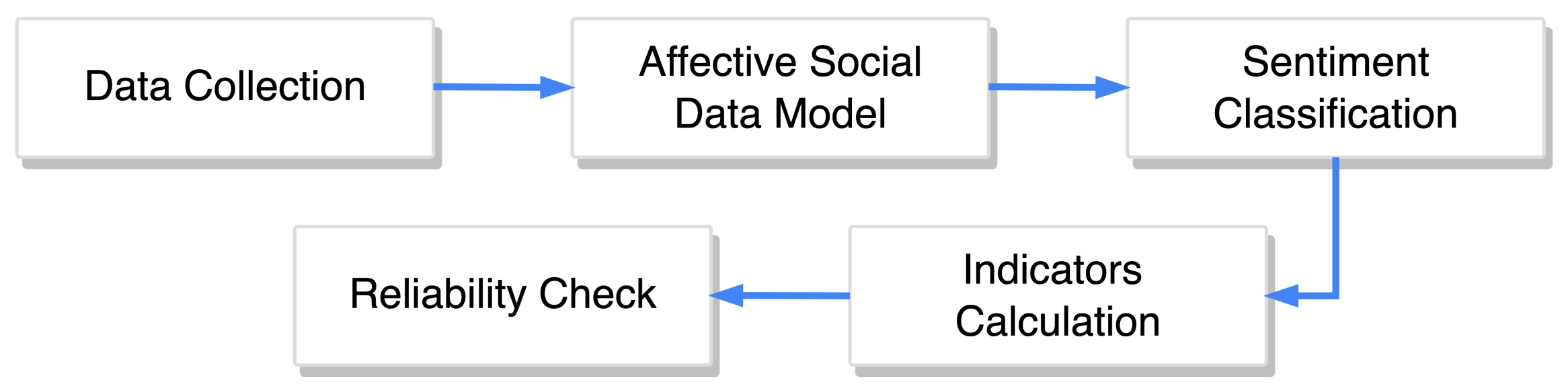
3. Measuring Observable Subjective Well-Being

The pipeline of the proposed approach (see Figure 1) consists of the following stages: obtaining raw data for analysis, training the sentiment classifier, building an affective social data model, selecting the OSWB metrics of interest, and calculating the OSWB indicators.

• Firstly, it is necessary to calculate the minimum sample size, and collect the required amount of data.
• Secondly, it is necessary to construct the affective social data model using collected data and sentiment classification model. The proposed affective social data model is based on the theory of socio-technical interactions (STI) [114] and the phenomenon of the social sharing of emotions (SSE) [80]. Online social network platforms involve individuals interacting with technologies and other individuals, thereby representing STI. When interacting, individuals tends to share their emotions (88–96% of emotional experiences are shared and discussed [80]) regardless of emotion type, age, gender, culture, and education level, though with slight variations between them [81]. Considering that emotional communication online and offline is surprisingly similar [84,85], we assumed both to be a good source for analyzing the affective state on the individual level and then aggregated it to capture the OSWB measure on the population level.
• Thirdly, the sentiment classification model should be trained to extract sentiment from the collected data. It is recommended to train the model on the training dataset from the same source as collected data. If the training dataset from the same source of data is not available, then it is recommended to select a training dataset from the most similar data source available.
• Fourthly, it is necessary to calculate OSWB indicators of interest using the constructed affective social data model. The proposed approach for calculation takes into account demographic characteristics of selected sample of users and maps this sample to the general population of the selected country via post-stratification.
• Lastly, the reliability of calculated indices must be verified. Among various available reliability measures, comparing the obtained OSWB indicators with existing survey-based SWB indicators tends to be the most straightforward option.

3.1. Data Sampling

A central idea behind data collection for computational social science research is collecting relatively inexpensive data, aiming at all the available data (i.e., big datasets are good, and bigger is better [115]). However, the question of determining the minimum sample size remains relevant. Following the standard approach from social sciences, the minimum sample size n and margin of error E are given by

$$x=Z{(c/100)}^2\times 2r(100-r)$$

(1)

$$n=N\frac{x}{(N-1)E^2+x},$$

(2)

$$E=\sqrt{\frac{(N-n)x}{n(N-1)}}$$

(3)

where N is the population size, r is the fraction of responses that you are interested in, and $Z(c/100)$ is the critical value for the confidence level c. When determining the sample size, one should also take into account the sample size used in classic survey-based SWB surveys. For example, Gallup World Poll typically uses samples of around 1000 individuals aged 15 or over in each country [56,116,117], the minimum sample size of World Values Survey is 1200 respondents aged 18 and older [118], and the regular sample size in Standard and Special Eurobarometer surveys is 1000 respondents per country [119]. In the case of Russian SWB surveys, the VCIOM Happiness index typically has samples of 1600 respondents aged 18 or over [40], and the FOM Mood of Others index has samples of 1600 respondents [120].

Note that in the case of working with electronic traces, the initial unit of analysis is digital trace, and there is often access not to the respondents directly, but to the traces that they left. The analysis of M electronic traces will not always mean that these traces were left by M users, and will depend on how many, on average, of the users leave traces. As a result, to estimate the minimum size of digital traces $n_{dt}$ it is additionally required to multiply the minimum number of respondents n on the average number of digital traces left by a user during analyzed time interval $\delta t$.

$$n_{dt}=n\times \delta t$$

(4)

However, in practice, it can be expected that prior to gaining access to digital traces, it is impossible to estimate the number of traces per user $\delta t$. In this case, after gaining access to as much data as possible, it will be enough to verify that these traces were left by a number of users that is not less than the calculated minimum number of respondents n.

3.2. Affective Social Data Model

The affective social data model for socio-technical interactions (see Definition 10) consists of two elements: actors and interactions. The actors (see Definition 11) represent participants of STI generating digital traces. The interactions (see Definition 12) represent structural aspects of STI and generated digital traces representing SSE. As a basis for the formal description of the model, we took the online social data model for social indicators research model that we proposed earlier [121] to analyze the influence of the misclassification bias on the social indicators research. We applied classical set theory to develop our model since the recent literature [122,123] articulated a series of its advantages in the computational social sciences.

Definition 1.

$U_{type}$ is a finite set of all user types defined as $U_{type}=\{individual,business\}$ where

• $Individual$ represents a user account which was created for personal use, and
• $business$ represents a user account which was created for business use.

It is important to delimit the types of accounts since the purpose of using a social network—and, as a result, the type of content—can strongly depend on them.

Definition 2.

$A{R}_{type}$ is a finite set of all artifact types defined as $A{R}_{type}=\{post,media,reaction\}$ where we have the following:

• $Post$ represents text and (or) media posts or comments;
• $Reaction$ represents the reactions to posted artifacts, such as likes or dislikes;
• $Media$ represents digital photos, videos, and audio content.

Each artifact type represents a type of user-generated content (UGC). Basically, $post$ represents all communications on users’ pages that occurs in the social networks, except private messages. (Our model does not consider private messages because not only are they extremely problematic to obtain, but their analysis can also raise a series of legal, privacy, and ethical questions.) Other UGC, such as digital photos, videos, and audio published in users’ albums, but not published on users’ pages, are represented as $media$. Reactions to $post$ and $media$, such as likes or dislikes, are represented as $reaction$.

Definition 3.

$SX$ is a finite set of sexes defined as $SX=\{male,female\}$ where

• $male$ represents male sex, and
• $female$ represents female sex.

Definition 4.

$BD$ is a set of birth dates.

Definition 5.

G is a set of geographical information.

Definition 6.

$MS$ is a finite set of marital statuses defined as $MS=\{married,single,divorced,widowed\}$ where we have the following:

• $Married$ represents a person who is in culturally recognized union between people called spouses;
• $Single$ represents a person who is not in serious committed relationships, or is not part of a civil union;
• $Divorced$ represents a person who is no longer married because the marriage has been dissolved;
• $Widowed$ represents a person whose spouse has died.

Definition 7.

$FT$ is a set of family types (i.e., classification of a person’s family unit) defined as $FT=\{nuclear,single-parent,blended,ofchoice\}$ where we have the following:

• $Nuclear$ represents a family which includes only the spouses and unmarried children who are not of age;
• $Single-parent$ represents a family of one parent (The parent is either widowed, divorced (and not remarried), or never married.) together with their children;
• $Blended$ represents a family with mixed parents (One or both parents remarried, bringing children of the former family into the new family.);
• $Ofchoice$ represents a group of people in an individual’s life that satisfies the typical role of family as a support system.

Definition 8.

$CN\in {\mathbb{N}}_0$ is the user’s numbers of children.

Definition 9.

$HS\in {\mathbb{N}}_0$ is the number of people living in the user’s household.

The combination of sex $SX$, birth date $BD$, marital states $MS$, family type $FT$, and number of children $CN$ represents demographics of the population and is of interest for conducting SWB studies [43]. This model does not consider other co-variates (e.g., material conditions, quality of life, and psychological measures) recommended for collection alongside measures of SWB since there is virtually no access to them within social networks data.

Definition 10.

The Affective Social Data Model for Socio-Technical Interactions is defined as a tuple $ASD{M}_{STI}=\{A,I\}$ where we have the following:

• A is the actors, representing the participants of socio-technical interactions generating UGC as defined further in Definition 11;
• I is the interactions, representing the structural aspects and UGC of $ASD{M}_{STI}$ as defined further in Definition 12.

As provided in the conceptual model and in Definition 10, the affective social data model for socio-technical interactions ($ASD{M}_{STI}$) contains actors (those who are doing and interacting) and interactions (what is being done and interacted).

Definition 11.

The Actors of $ASD{M}_{STI}$ is defined as a tuple $A=(U,U_{type},SX,BD,MS,FT,CN,HS,G,f_{U_{type}}^U,f_{S?}^U,f_{BD?}^U,f_{MS?}^U,f_{FT?}^U,f_{CN?}^U,f_{HS?}^U,f_{G?}^U)$ where we have the following:

• U is a finite set of users ranged over by u;
• $U_{type}$ is a finite set of user types (as defined in Definition 1) ranged over by $u_{type}$;
• $SX$ is a finite set of users’ sexes (as defined in Definition 3) ranged over by $sx$;
• $BD$ is a set of users’ birth dates ranged over by $bd$;
• $MS$ is a set of users’ marital statuses (as defined in Definition 6) ranged over by $ms$;
• $FT$ is a set of users’ family types (as defined in Definition 7) ranged over by $ft$;
• $CN$ is the user’s numbers of children (as defined in Definition 8) ranged over by $cn$;
• $HS$ is a set of numbers of people living in the users’ households (as defined in Definition 9) ranged over by $hs$;
• G is a set of users’ geographical information (as defined in Definition 5) ranged over by g;
• $f_{U_{type}}^U:U\to U_{type}$ is the user type function mapping each user to the user type;
• $f_{S?}^U:U\to S$ is the sex function mapping each user to the user’s sex if defined;
• $f_{BD?}^U:U\to BD$ is the birth date function mapping each user to the user’s birth date if defined;
• $f_{MS?}^U:U\to MS$ is the marital status function mapping each user to the user’s marital status if defined;
• $f_{FT?}^U:U\to FT$ is the family type function mapping each user to the user’s family type if defined;
• $f_{CN?}^U:U\to CN$ is the number of children function mapping each user to the user’s number of children if defined;
• $f_{HS?}^U:U\to HS$ is the household size function mapping each user to the user’s household size if defined;
• $f_{G?}^U:U\to G$ is the geographic information function mapping each user to the user’s geographic information if defined.

The formal definition of actors is provided in Definition 11. The first two items contain a set of users (U) and a set of user types ($U_{type}$), respectively. The next six items contain demographic information, including sex ($SX$), birth date ($BD$), marital status ($MS$), family type ($FT$), the numbers of children ($CN$), the numbers of people living in the household ($HS$), and geographical information (G). The rest of the items are mapping functions from a user to the user’s type and all mentioned demographic characteristics if defined. The set of demographic characteristics was constructed based on existing guidelines on measuring SWB [43,56,58,70] to cover as many potentially useful demographic data as possible, although we understand that some of them can be unavailable in digital trace data (see Definition 8).

Definition 12.

The Interactions of $ASD{M}_{STI}$ is defined as a tuple $I=(AR,A{R}_{type},S,f_{U_{feed}}^{AR},f_{U_{author}}^{AR},f_{A{R}_{type}}^{AR},f_{AR}^{AR},f_S^{AR},trac{k}_T^{U,AR},ag{e}_{AR}^U:trac{k}_T^{U,AR},{\to }_{post},{\to }_{react})$ where we have the following:

• $AR$ is a finite set of artifacts ranged over by $ar$;
• $A{R}_{type}$ is a finite set of artifact types (as defined in Definition 2) ranged over by $a{r}_{type}$;
• S is a finite set of sentiment classes ranged over by s. (The list of final classes is not specified within this model, since it is expected that it may differ both depending on the final task of building the index and depending on the markup of the training dataset that is used to train the model.)
• $f_{U_{feed}}^{AR}:AR\to U$ is a function mapping the artifact and the user on whose feed it was published;
• $f_{U_{author}}^{AR}:AR\to U$ is a function mapping the artifact and the user created it;
• $f_{A{R}_{type}}^{AR}:AR\to A{R}_{type}$ is the artifact type function mapping each artifact to an artifact type;
• $f_{AR}^{AR}:AR\to AR$ is a parent artifact function, which is a partial function mapping artifacts to their parent artifact if defined;
• $f_S^{AR}:AR\to S$ is a relation defining mapping between artifact and sentiment;
• $trac{k}_T^{U,AR}:(U\times AR)\to N$ is a time function that keeps tracks of the timestamp of an artifact created by an user;
• $ag{e}_{AR}^U:trac{k}_T^{U,AR}\times f_{BD?}^U\to N?$ is a time function that returns the age of the user on the time of the artifact creation if the user’s birthday is defined;
• ${\to }_{post}:U\to P_{disj}\left(AR\right)$ is a partial function mapping users to mutually disjoint sets of their artifacts;
• ${\to }_{react}:U\to P\left(AR\right)$ is a partial function mapping users to the artifacts reacted by the users.

3.3. Sentiment Classification

As can be seen from $ASD{M}_{STI}$ definition, S represents a finite set of sentiment classes, and $f_S^{AR}$ represents mapping between an artifact and a sentiment. From the sentiment classification perspective, S is a set of classes in a training sentiment dataset, and $f_S^{AR}$ is a function that runs the sentiment classification model trained on the sentiment dataset and returns the sentiment of the artifact.

3.4. OSWB Indicator Calculation

The approach for calculating OSWB indicators consists of three steps.

• Select content of interest for the analysis; that is, textual posts published by users on their own pages.
• Make data sample representative of the target population by applying sampling techniques.
• Calculate selected OSWB measures based on the representative data sample.

3.4.1. Data Selection

Definition 13.

$TI=\{t{i}_1,t{i}_2,\dots ,t{i}_T\}$ is a finite ordered set of T non-overlapping time intervals, such as $t{i}_i<t{i}_{i+1}$.

Definition 14.

${\to }_{interval}:(ag{e}_{AR}^U:trac{k}_T^{U,AR}\to N?)\to TI?$ is a partial mapping a timestamp of artifact creation to a time interval if the birthday of the user is defined.

Definition 15.

P is a finite set of $PN$ textual posts published by users on their own pages and defined as follows:

$$\begin{array}{c}\hfill P=\left\{ar\right|f_{A{R}_{type}}^{AR}\left(ar\right)=post|\forall ar\in AR\wedge f_{U_{feed}}^{AR}\left(ar\right)=\\ \hfill f_{U_{author}}^{AR}\left(ar\right)\wedge f_{UBD?}\ne ⌀\wedge f_{AR}^{AR}\left(ar\right)=⌀\}\end{array}$$

(5)

Definition 16.

$P_{t{i}_i}$ is a finite set of $P{N}_{t{i}_i}$ posts published by authors on their pages during time interval $ti$ and is defined as follows:

$$\begin{array}{c}\hfill P_{t{i}_i}=\left\{p\right|\forall p\in P\wedge {\to }_{interval}\left(p\right)=t{i}_i\},\sum _{i=1}^{T}P{N}_{t{i}_i}=PN\end{array}$$

(6)

We focus on the user’s own posts posted on their pages, as we assume that such posts are more likely to contain the emotional state of the author compared to posts elsewhere. We also believe that the users’ pages in most cases are not limited to a specific thematic domain, in comparison with the walls of groups and communities; therefore, these posts should contain a larger number of different topics and, on average, be general-domain sources of data.

Definition 17.

$\dot{U_{t{i}_i}}$ is a finite set of users who posted textual posts on their own profiles within time interval $ti$ and is defined as follows:

$$\dot{U_{t{i}_i}}=\left\{f_{U_{author}}^{AR}\left(p\right)\right|\forall p\in P_{t{i}_i}\}$$

(7)

After obtaining $\dot{U_{t{i}_i}}$, it is necessary to validate that the number of users for each time interval $t{i}_i$ is not less that the minimum sample size n (see Equation (2)). In case it is less than n for at least one $t{i}_i\in TI$, then the calculation of the index with the selected confidence level and margin of error is not possible.

3.4.2. Data Sampling

Definition 18.

$\dot{DF}$ is a finite set of $DFN$ demographics mapping functions with defined values over the given users set and is defined as follows.

$$\begin{array}{c}\hfill \dot{DF}=\left\{f\right|\forall f\in \{f_{S?}^U,ag{e}_{AR}^U,f_{MS?}^U,f_{FT?}^U,f_{CN?}^U,f_{HS?}^U,f_{G?}^U\},\\ \hfill \wedge f\left(u\right)\ne ⌀,\forall u\in U\}\end{array}$$

(8)

Since not all of these characteristics can be obtained from social network data, in accordance with the European Social Survey Sampling Guidelines [58], it is recommended to use at least age and gender characteristics for the sampling design.

Definition 19.

$\ddot{U_{t{i}_i}}$ is a finite set of users $\dot{U_{t{i}_i}}$ representative of the target population by applying stratification (Here, $N_{t}p$ is the population size, n is the total sample size, k is the number of strata, $N_i$ is the number of sampling units in i-th strata such as ${\sum }_1^k{N}_i=N$, $n_i$ is the number of sampling units to be drawn from i-th stratum such as ${\sum }_1^k{n}_i=n$. Strata are constructed such that they are non-overlapping and homogeneous with respect to the characteristic under study. For fixed k, the proportional allocation of stratum size can be calculated as $n_i=\frac{n}{N}{N}_i$, where each $n_i$ is proportional to stratum size $N_i$.) by $\dot{DF}$.

Definition 20.

$\dot{P_{t{i}_i}}$ is a finite set of posts created by representative sample of users $\ddot{U_{t{i}_i}}$ on their own pages during time interval $ti$ and defined as follows:

$$\dot{P_{t{i}_i}}=\left\{p\right|\forall p\in P_{t{i}_i}\wedge f_{U_{author}}^{AR}\left(p\right)\in \ddot{U_{t{i}_i}}\}$$

(9)

3.4.3. Index Calculation

Firstly, it is required to aggregate sentiment for users who posted several times during the considered time intervals.

Definition 21.

$ag{g}_{u,t{i}_i}$ is the sentiment aggregation function which aggregates the sentiment of posts published during time interval $t{i}_i$ by user u and is defined as follows:

$$ag{g}_{u,t{i}_i}:P\times P\to S$$

(10)

The aggregation function can be defined in several ways (e.g., major voting).

Definition 22.

$AU{S}_{t{i}_i}$ is the aggregated user sentiment expressed in a post published during $t{i}_i$ period of time.

$$\begin{array}{c}\hfill AU{S}_{t{i}_i}=\{ag{g}_{u,t{i}_i}\left(\right(f_S^{AR}\left(p_0^u\right),(f_S^{AR}\left(p_1^u\right),(f_S^{AR}(\dots ),\\ \hfill (f_S^{AR}(p_j^u))|\forall p^u\in \dot{P_{t{i}_i}},\forall u\in \ddot{U_{t{i}_i}}\wedge f_{U_{author}}^{AR}(p^u)=u\}\end{array}$$

(11)

Finally, the OSWB indicator can be calculated.

Definition 23.

$OSWB{I}_{t{i}_i}$ is the OSWB indicator and is defined as follows:

$$OSWB{I}_{t{i}_i}=\{indicator\left(aus\right)|\forall aus\in \dot{AU{S}_{t{i}_i}}\}$$

(12)

where $indicator$ is an indicator formula, which can be defined in several ways depending on the study goals (see examples in Section 4.5).

4. Observable Subjective Well-Being Based on Odnoklassniki Content

4.1. Odnoklassniki Data

According to the VCIOM survey [124] in 2017, the preferences among usage of particular social networks in Russia have age characteristics. The largest share of the audience of VKontakte users, 40% of the total audience, consists of people aged 25–34 years. Among Instagram users, 38% are between the ages of 18 and 24, and 37% are between the ages of 25 and 34. Among the daily audience of Odnoklassniki, the most common group is also 25–34 years old (28%). At the same time, the distribution of the Odnoklassniki audience by age is the closest among all social networks to the general distribution of the internet audience in Russia [124]. Similar findings were reported in the study by [125], where the author concluded that Odnoklassniki is the most democratic social network in Russia because it is used by all categories of the population, including “traditional non-users”—that is, the elderly and people with a low level of education. In fact, according to Brodovskaya, the only network used by older Russians is Odnoklassniki, since Russians who have reached the age of 60 do not have accounts on any foreign social networks. This makes Odnoklassniki a great source of data for analysis since post-stratification weights are not expected to vary significantly. In case some subgroups have either extremely small or extremely large weights, it can actually make the estimate worse by increasing the model’s variance and sensitivity to outliers [126].

We calculated the minimum sample size (see Section 3.1) using Raosoft (http://www.raosoft.com/samplesize.html, accessed on 1 May 2022) (population size of 40,000,000 [127], the same margin of error of 2.5% and confidence level of 95% as was used in VCIOM Happiness [40]) and yielded $n=1537$. Considering that we did not have information about average number of posts by users, we requested from the OK Data Science Lab as many posts as they could provide, but not fewer than 1537 per day. We requested only those posts which (1) contained textual content only, (2) were published by individual users on their own public pages, and (3) were published within the territory of Russia.

The OK Data Science Lab provided us with 7,200,000 randomly selected textual (i.e., $\forall ar\in AR,f_{A{R}_{type}}^{AR}\left(ar\right)=post$) posts published in Russia (i.e., $\forall u\in U,f_{G?}^U\left(u\right)=Russia$) by individual users (i.e., $\forall u\in U,f_{U_{type}}^U\left(u\right)=individual$) on their public profiles between April 2020 and May 2021, for a total of 20,000 posts per day. Each post contained anonymized user identifiers (primary identifier of artifacts $ar\in AR$), date of birth if known ($bd\in BD$), gender if known ($sx\in SX$), time of publication (required for ${\to }_{interval}$), author’s time zone at the moment of publication (required for ${\to }_{interval}$), author’s country ($f_{G?}^U\left(u\right)=Russia$ for all posts) at the moment of publication (based on IP and other Odnoklassniki internal heuristics (the quality of determining geolocation by IP is outside of the scope of this work)), text (required for sentiment mapping function $f_S^{AR}$), and language used in the post. We then filtered out duplicates, posts of authors without date of birth or gender, and obtained 7,049,907 posts for further analysis. These posts were published by 3,610,891 unique users—1.95 posts per user on average. We checked the number of unique authors of posts for each day and confirmed that it exceeds 1537 unique authors for each day. All user data were provided in an anonymized format; therefore, it was impossible to identify the real author of the post. A more detailed description of the characteristics of the data (e.g., gender and age distribution) is not possible in accordance with the Non-Disclosure Agreement; however, it is available through official Ondoklassniki reports [127] (see

Table 1. Gender distribution for Odnoklassniki audience in 2021. Source: [127].

Age Group	Audience
	Female	Male
17	2%	1%
18–24	4%	2.8%
25–34	11%	8.2%
35–44	15%	10.8%
45–54	12%	7.3%
55–64	11%	5.3%
65+	7%	3.4%

). The core of the Ondoklassniki audience is women and men 25–44 [128]. All generations of people are represented in Ondoklassniki: children, teenagers, the core of the audience aged 25–44, and older people.

The Odnoklassniki data are available from OK Data Science Lab, but restrictions apply to the availability of these data; they were used under license for the current study, and so they are not publicly available. Data are, however, available from the OK Data Science Lab upon reasonable request, https://insideok.ru/category/dsl/ (accessed on 1 May 2022).

4.2. Demographic Groups

While selecting demographic groups, in addition to general guidelines on measuring SWB mentioned earlier [43,56,57,58], we also relied on recommendations by Russian research agencies to cover country-specific aspects: the VCIOM SPUTNIK methodology [129] and RANEPA Eurobarometer methodology [130]. Thus, we selected the following demographic variables for post-stratification.

• Gender. The array reflects the sex structure of the general population: male and female.
• Age. The array is divided into four age groups, reflecting the general population: 18–24 years old, 25–39 years old, 40–54 years old, and 55 years old and older.

While the model contains many other demographic characteristics (e.g., $FT$, $CN$, $HS$, G from Definition 11), we were unable to use them to construct the OSWB indices because the Odnoklassniki data did not contain them.

The data about real population characteristic were obtained from the Federal State Statistics Service of Russia (https://rosstat.gov.ru/compendium/document/13284, accessed on 1 May 2022).

4.3. Sentiment Classification

4.3.1. Training Data

Manual annotation of a subset of provided Odnoklassniki posts via crowdsourcing platforms was not possible in accordance with the non-disclosure agreement. Thus, for training a classifier, we chose one of the existing datasets with the data that are most similar to posts from Odnoklassniki. Unfortunately, the Russian language is not as well resourced as the English language, especially in the field of sentiment analysis [65], so the selection options were quite limited. Based on the previously obtained list of available training datasets in Russian [37], we identified RuSentiment [39], which consists of posts from VKontake (VKontake is the largest national social network in Russia, with about 100M active users per month [131]), as the most appropriate dataset due to the following reasons. Firstly, RuSentiment is the largest sentiment dataset of general-domain posts in Russian, which was annotated manually (Fleiss’ $\kappa =0.58$) by native speakers with linguistic background. Almost all other datasets are either domain-specific (e.g., SentiRuEval 2016 [132]) or annotated automatically (e.g., RuTweetCorp [133]), or both (e.g., RuReviews [134]). The only exception is the RuSentiTweet [135] dataset, but it consists from Russian-language tweets and as a result, has different linguistic characteristics. Secondly, the corpora similarity measure proposed by Dunn [136] confirmed that RuSentiment and Odnoklassniki data are similar (see Appendix A for details). The similarity between texts from Odnoklassniki and VKontakte was intuitively expected since they are the two largest national social networks in Russia [137], very close in terms of the available functionality for communications [138], and used by Russians with approximately the same intensity [125].

RuSentiment contains 31,185 general-domain posts from Vkontakte (28,218 in the training subset and 2967 in the test subset), which were manually annotated into five classes:

• Positive Sentiment Class represents explicit and implicit positive sentiment.
• Negative Sentiment Class represents explicit and implicit negative sentiment.
• Neutral Sentiment Class represents texts without any sentiment.
• Speech Act Class represents congratulatory posts, formulaic greetings, and thank-you posts.
• Skip Class represents noisy posts, unclear cases, and texts that were likely not created by the users themselves.

The dataset was labeled by native speakers with a linguistics background with a Fleiss’ kappa of 0.58. The dataset consists of two subsets: training subset (28,218 texts) and test subset (2967 texts). We trained our models on the training subset and reported classification metrics on the tests subset to compare results with other studies on RuSentiment.

4.3.2. Classification Model

Based on the literature review, we selected the following pretrained language models for fine-tuning experiments to identify the most accurate one.

• XLM-RoBERTa-Large (https://huggingface.co/xlm-roberta-large, accessed on 1 June 2022) [107] by Facebook is a multilingual RoBERTa [139] model with BERT-Large architecture trained on 100 different languages.
• RuRoBERTa-Large (https://huggingface.co/sberbank-ai/ruRoberta-large, accessed on 1 June 2022) [113] by SberDevices is a version of the RoBERTa [139] model with BERT-Large architecture and BBPE tokenizer from GPT-2 [140] trained on Russian texts.
• mBART-large-50 (https://huggingface.co/facebook/mbart-large-50, accessed on 1 June 2022) [108] by Facebook is a multilingual sequence-to-sequence model pretrained using the multilingual denoising pretraining objective [141].
• RuBERT (https://huggingface.co/DeepPavlov/rubert-base-cased, accessed on 1 June 2022) [105] by DeepPavlov is a BERT model trained on news data and the Russian-language part of Wikipedia. The authors built a custom vocabulary of Russian subtokens and took weights from the Multilingual BERT-base as initialization weights.

The characteristicsof the selected models, including information about tokenization, vocabulary, and configuration, can be found in

Table 2. Characteristics of selected models.

Model	Vocabulary			Configuration
	Tokenization	Size	Cased	Size	Parameters
XLM-RoBERTa-Large	SentencePiece	250 K	yes	large	560 M
RuRoBERTa-Large	Byte-level BPE	50 K	yes	large	355 M
MBART-50-Large	SentencePiece	250 K	yes	large	611 M
RuBERT	WordPiece	101 K	yes	base	178 M

.

On the top of the pretrained language model, we applied a simple softmax layer to predict the probability of classes c:

$$p\left(c\right|h)=\mathrm{softmax}(Wh),$$

(13)

where W is the task-specific parameter matrix of the added softmax layer. The fine-tuning stage was performed on 1 Tesla V100 SXM2 32GB GPU with the following parameters: a number of train epochs of [4, 5, 6, 7, 8], a max sequence length of 128, a batch size of [16, 32, 64], and a learning rate of [2e-6, 2e-5, 2e-4]. The hyperparameter value ranges were chosen based on values used in existing studies [65,105,135,142,143]. Fine-tuning was performed using the Transformers library [144]. Since the dataset originally had a division into test and training subsets, we additionally divided the existing training subset into validation (20%) and new training (80%) subsets. The models were evaluated in terms of macro $F_1$ and weighted $F_1$ measures:

$$macro{F}_1=\frac{1}{N}\sum _{i=1}^N{F}_{1,i}$$

(14)

$$weighted{F}_1=\frac{1}{N}\sum _{i=1}^N{W}_i\ast F_{1,i}$$

(15)

where i is the class index, N the number of classes, and $W_i$ is the weight of class i. The highest possible value of macro and weighted $F_1$ is 1.0 and the lowest possible value is 0. We repeated each experiment 3 times and reported the mean values of the measurements.

According to the results of fine-tuning presented in

Table 3. Classification results of fine-tuned models. Random represents a random classifier. Weighted $F_1$ is reported because it was used as the main quality measure in the original paper. Existing weighted $F_1$ SOTA was achieved by shallow-and-wide CNN with ELMo embeddings [145]. Existing macro $F_1$ SOTA was achieved by fine-tuned RuBERT [65].

Model	Measure
	Macro ${\mathit{F}}_1$	Weighted ${\mathit{F}}_1$
Random	18.56	23.00
Existing SOTA	72.03	78.50
XLM-RoBERTa-Large	75.67	78.69
RuRoBERTa-Large	76.30	78.92
mBART-large-50	68.63	72.88
RuBERT	71.91	75.49

, RuRoBERTa-Large ($n_{epoch}=4$, $lr=2e-5$, $bs=64$) demonstrated the best classification scores of weighted $F_1=76.30$ (4.27 percentage points above existing SOTA) and macro $F_1=78.92$ (0.42 percentage points above existing SOTA), thereby achieving new state-of-the-art results on RuSentiment. XLM-RoBERTa-Large ($n_{epoch}=4$, $lr=2e-5$, $bs=32$) showed slightly lower but still competitive results. However, taking into account that XLM-RoBERTa-Large is larger than RuRoBERTa-Large, it turns out that in any case, it is much more efficient to use RuRoBERTa-Large for sentiment analysis of RuSentiment data. Surprisingly, mBART-large-50 ($n_{epoch}=5$, $lr=2e-5$, $bs=16$) did not show results higher than those of RuBERT ($n_{epoch}=4$, $lr=2e-5$, $bs=64$).

The most common misclassification errors of RuRoBERTa-Large (see Figure 2) were the classifying Skip Class as Neutral and Positive Class, Negative Class as Neutral Class, and Neutral Class as Positive. The speech acts class was more clearly separated from other classes because it was composed of a well-defined group of speech constructs. Predictably, the Skip Class was one of the most hardly classified because this class initially contained noisy and hardly interpretable posts. Neutral sentiment is logically located between negative and positive sentiment, so it is expected that it can be classified incorrectly. As was mentioned in our previous study [65], this issue looks like a general challenge of non-binary sentiment classification. For example, Barnes et al. [146] also reported that the most common errors come from the no-sentiment classes (i.e., the Neutral Class in our case).

We made the fine-tuned RuRoBERTa-Large model publicly available (https://github.com/sismetanin/sentiment-analysis-in-russian, accessed on 1 May 2022) to the research community.

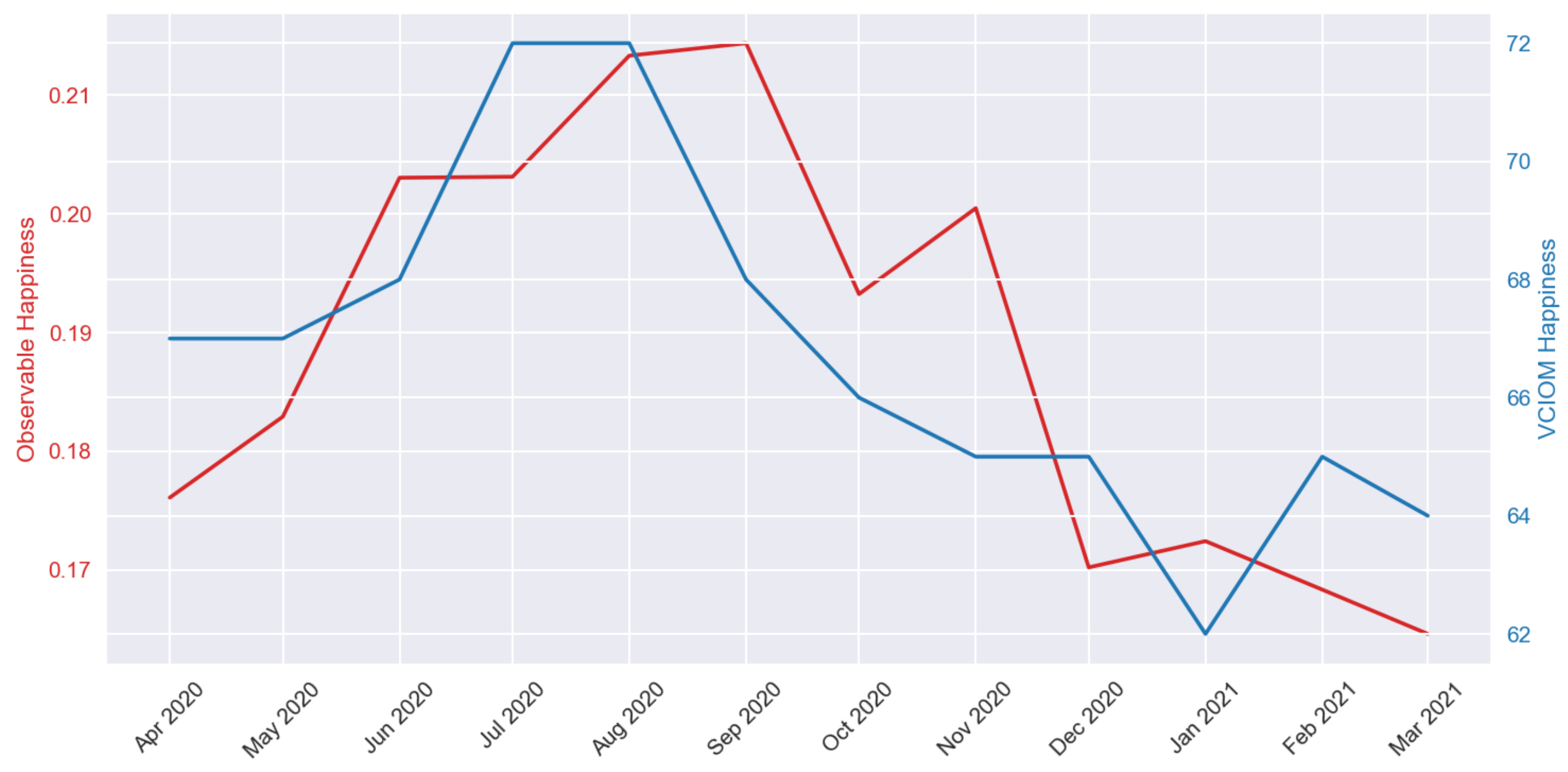
4.4. Validity Check

As mentioned in the literature review, according to the OECD Guidelines on Measuring SWB [43], validity can be verified by comparing results when using different measures on the individual level. However, this implies that for verification, we need the SWB values of the indicator obtained by the classical survey method for at least a part of the study participants. Of course, we do not have such data at our disposal; however, in earlier literature [147] it was indicated that the language-based assessment of social media posts can constitute valid SWB measures. Thus, to verify the results in our case, we propose to check the validity on the aggregated level by selecting an existing indicator obtained on the basis of survey data, which will coincide in the time period with our indicator. Considering that our time period is relatively small, we cannot use an indicator that is calculated once a year since it makes no sense to build a correlation based on a time series of two values. Among the SWB indices for Russia, calculated by the organizations mentioned in the literature review, the VCIOM Happiness index seems to be best suited for our time period since it was calculated monthly. Thus, for the reliability check, we decided to use the VCIOM Happiness index. Validity checks for OSWB studies at the aggregate level have also been used in other studies (e.g., [29,148]), so we followed their practice.

4.5. Indicator Formula

Within our study, we explored two types of indicator formulas.

Definition 24.

$OSW{B}_{PA}$ is the observable positive affect indicator (experiencing pleasant emotions and moods) and is defined as follows:

$$OSW{B}_{PA}=\frac{POS}{POS+NEG+NEU+SA+SKIP}$$

(16)

where $POS$ is the number of positive posts, $NEG$ is the number of negative posts, $NEU$ is the number of neutral posts, $SA$ is the number of posts with greetings and speech acts, and $SKIP$ is the number of ambiguous posts that cannot be unambiguously assigned to one of the other classes.

The indicator takes values from 0 to 1.

Definition 25.

$OSW{B}_{NA}$ is the observable negative affect indicator (experiencing unpleasant, distressing emotions and moods) and is defined as follows:

$$OSW{B}_{NA}=\frac{NEG}{POS+NEG+NEU+SA+SKIP}$$

(17)

The indicator takes values from 0 to 1.

4.6. Misclassification Bias

Although we achieved new SOTA results on the RuSentiment dataset, the best classification model was still not error-free, which could introduce a bias in our analysis results. To estimate the impact of misclassification bias on OSWB indicators of interest, we applied a simulation approach for misclassification bias assessment introduced in our previous paper [121]. For the generation of synthetic time series, we applied Nonlinear Autoregressive Moving Average model from the TimeSynth [149] library with random hyperparameters for each simulation run. We chose Pearson’s and Spearman’s correlation coefficients as the main metrics. For each indicator calculated further (see Section 4.5), we ran 500,000 simulation iterations. According to the results of the simulation, the aggregated p-values are higher than 0.95, and both coefficients demonstrated almost perfect aggregated correlation scores. Thus, we can confirm that the there is a negligible impact of the misclassification bias on the calculation of all considered indices, allowing us to achieve an almost perfect level of correlation between the predicted and true underlying indicators.

5. Results

We calculated the observable happiness indicators for each month for a period from April 2019 to March 2021 (12 months) and found (Normality was tested using the Shapiro–Wilk test since it is the most suitable for small sample sizes [150]. Stationarity was tested using KPSS and Dickey–Fuller GLS tests since these tests are the most appropriate for our small sample size [151]. Homoscedasticity was tested using the White test [152]. Our approach for measuring correlation is the same as the approaches used in the existing literature on SWB—for example [73,153].) moderate to strong (depending on the interpretation guidelines [154]) Pearson’s linear correlation ($r=0.733$, $p=0.007$) and strong Spearman’s monotonic correlation ($r_s=0.825$, $p=0.001$) between $OSW{B}_{PA}$ (further referred to as Observable PA) and the VCIOM Happiness index. Since previous studies reported that the typical reliability of SWB scales is in the range from 0.50 to 0.84 [21,41,42,44,45] (and even between 0.40 and 0.66 for single-item measures, such as VCIOM Happiness [42]), we can consider obtained correlation as practically close to unity. Interestingly, $OSW{B}_{NA}$ (further referred to as observable NA) showed no statistically significant correlation with the VCIOM index. Considering that observable PA showed a positive correlation, one may suppose that observable NA might be negatively correlated with the VCIOM Happiness indicator; however, that hypothesis was not confirmed. We assume that this could happen for at least two reasons. Firstly, this could be due to the fact that the share of negative posts does not really correlate with the subjective well-being of the respondents. Secondly, this could also be due to the fact that there were much fewer negative posts than positive ones, and to see the correlation between observable NA and the VCIOM Happiness indicator, we need to work with a larger dataset.

As can be seen in Figure 3, Observable PA and VCIOM Happiness indicators are quite similar. Both indicators demonstrated growth in the beginning of the analysed period and rapid decline starting from Autumn 2020. According to the OECD Guidelines on Measuring SWB [43], a cut-off at 0.7 is considered an acceptable level of internal consistency reliability for tests based on comparing results when using different measures, so we can confirm an acceptable level of reliability for our approach. However, given the sample size on which the study was conducted, the conclusion about the validity is most likely of a preliminary nature. For unambiguous confirmation of validity, it is necessary to test the correlation on more data, which was not possible in this study.

Previous research has consistently shown the existence of circadian (24 h) and circaseptan (7 day) patterns in humans [155], so in Section 5.1 and Section 5.2, we explore changes in observable PA on a daily and weekly basis in more detail.

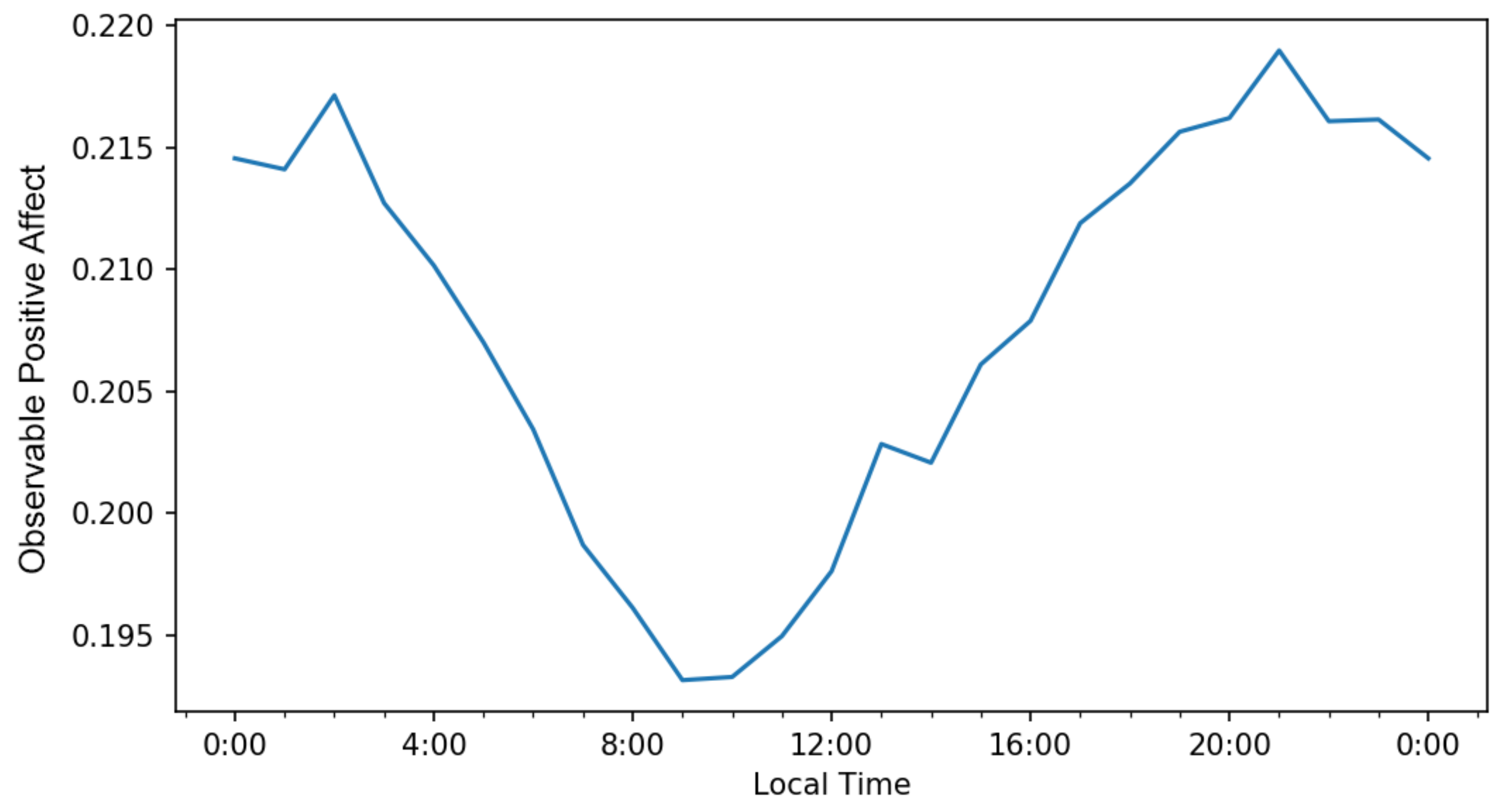
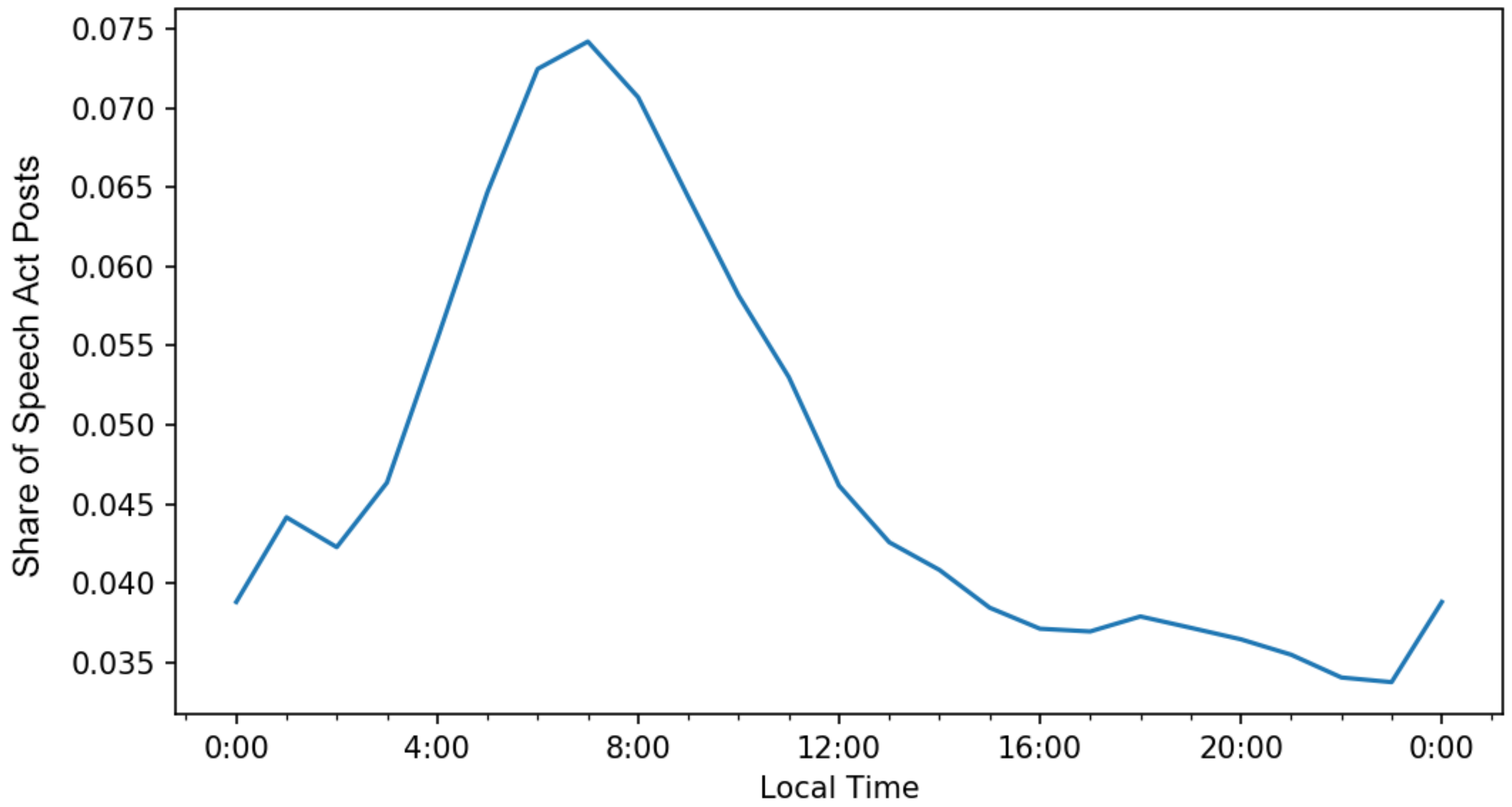
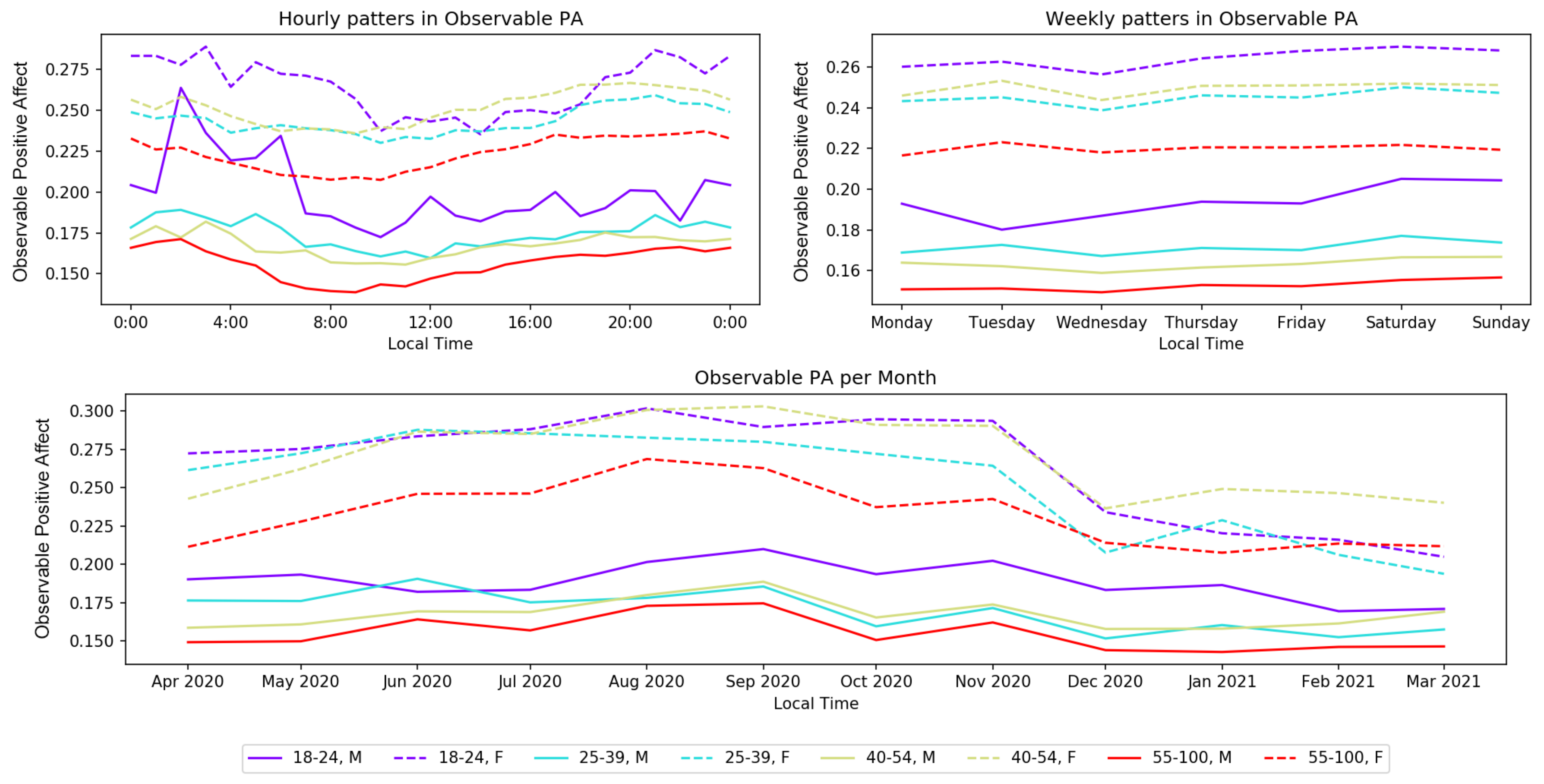
5.1. Daily Patterns

General daily variations can be clearly seen (see Figure 4), with morning having the lowest level of happiness and late evening having the highest. The obtained general daily patterns differ from the patterns reported in other OSWB studies (e.g., [24,32]), since in the majority of cases, two spikes were previously reported: one in the early morning and the other in the late evening. In our case, we assume that we did not have early morning spike due to both methodological and geographical aspects. From the methodological point of view, we deliberately did not consider greetings and speech acts as a manifestation of positive emotions and treated them as a separate class instead. The key reason behind this decision is that greetings and speech acts make use of sentiment (commonly positive) related words while not necessarily denoting the the underlying sentiment of the author [39,156]. In addition, greetings and speech acts commonly consist of a limited set of speech structures and expressions (e.g.,“Good morning” posts), so they are much more clearly distinguishable from other classes. For example, RuRoBERTa achieved $F_1=0.94$ for speech acts class and only $F_1=0.77$ for positive class. Thus, in the case of treating greeting and speech act posts as positive, the signal about mood could be skewed by the presence of large amounts of clearly distinguishable greetings and speech acts [156]. We assume that this is why other studies have reported peaks at the start of the day: because this is where the highest number of greeting and speech act posts occur (see Figure 5). From the geographical point of view, the presence of different time zones within the same country (for example, Russia has 11 time zones) makes it more difficult to compare patterns between countries and may cause differences in patterns for these countries. In contrast with other studies, we analyzed the local time of each timezone: posts published at 12:00 a.m. GMT+3 and 12:00 a.m. GMT+5 were treated as posts published at 12:00 a.m. local time, which allowed us to measure daily patterns more accurately. The absence of early morning spikes perfectly corresponds to the results of classical survey-based study conducted by Cornelissen et al. [157]. The authors built a positive affect indicator, which in shape completely coincides with the graph obtained in our study: the lowest point is reached in the morning, then the graph grows up to 18 h and begins to fall closer to night. The key difference is that our indicator is shifted by a few hours to the right relative to their indicator (e.g., the lowest point on their indicator is reached at 6:00 a.m., and on ours at 8:00 a.m.). We suppose that this difference arose due to the discrepancy between the samples under consideration since they surveyed only students, and our study targeted the larger number of demographic groups. A similar pattern can be observed in another study [158] which reported net affect and positive affect measures for Russia. The authors reported that net affect and positive affect improved as the day passed, with the lowest point around 9:00 a.m., which corresponds with our results.

5.2. Weekly Patterns

Weekly patterns in OSWB can be clearly observed as well (see Figure 6), with weekends being happier than weekdays. At the level of individual days of the week, we can also observe the previously described daily patterns, which have different amplitudes and extremes depending on a particular day. During the week, the lowest level of happiness occurs in the first three weekdays, and starting on Thursday it starts to rise and peaks at the weekend. Russians wake up in their best mood on Saturday and reach their highest level of happiness closer to the night. These weekly patterns are intuitively expected, since as was mentioned by Mayor and Bietti [155], weekly patterns are generally associated with cultural traditions and the cultural distinction between weekdays and weekends in modern societies regulating social practices and behaviors. Similar results were reported for other countries both in the framework of traditional sociological research (e.g., [159,160]) and research based on digital traces (e.g., [24,156]).

5.3. Demographic Patterns

Although different demographic groups generally follow common patterns, they have different levels of happiness over the analyzed time periods. For example, the level of observable PA tends to decline over increasing age for both men and women. This finding is supported by a series of results from other Russian studies on this problem [161], where the authors also confirmed that the subjective assessment of well-being is associated with age: the subjective assessment of well-being is higher in young groups and decreases in older groups. Additionally, the data show that women not only have higher levels of observable PA relative to men within the same age group, but they generally show higher levels of observable PA than men. However, it is important to take into account the specifics of the data under study and be careful when making conclusions about which of the demographic groups is actually happier. First, it should be noted that different demographic groups have not only different patterns of using social networks, but also sharing information and emotions. In other words, based on these graphs, it is possible to construct not only a hypothesis about higher level of women’s happiness, but also that women are more actively sharing positive emotions on social networks. However, the verification of these hypotheses lies outside the scope of this study, and, in our opinion, is of great scientific interest for future work. Despite the possible options for the interpretation of the data obtained, the differences found in demographic groups nevertheless confirm the need to apply classical sociological research practices in OSWB research, such as the construction of representative samples and/or post-stratification.

6. Discussion

Observable PA demonstrated a high level of correlation with the VCIOM Happiness index, indicating its reliability. As can be seen from the existing literature [21,41,42,43,44,45], the typical reliability of SWB scales is in the range of 0.50 to 0.84. In case of single-item measures, such as VCIOM Happiness [42], the reliability is even between 0.40 and 0.66 [42]. Thus, it seems that our results can be interpreted as almost perfect correlation. The results of daily pattern analysis generally agree with the findings of other survey-based SWB studies [157,158], but they differ from the results of OSWB studies [24,32] for other countries, since they commonly reported a positive spike in the morning. The difference with other OSWB studies can be explained by several factors: treating greetings and speech acts as a separate class (not positive class as in other studies) and calculating index in local time for each time zone since we had access to the user’s time zone (see Section 5.1 for details). We hypothesize that the positive morning spikes reported by other studies are precisely associated with a high proportion of greetings and speech acts. As was highlighted by Refs. [39,156], greetings and speech acts make use of sentiment (commonly positive) related words, while not necessarily denoting the the underlying sentiment of the author, and may be expressed under the social pressure. Considering that our daily patterns corresponds to other survey-based SWB studies, we argue that greetings and speech acts should not be considered as a positive sentiment class in OSWB research. As for the weekly pattern, we clearly saw that weekends have higher levels of observable PA than weekdays. This result agrees with existing survey-based SWB [159,160] and OSWB [24,156] studies, since weekly patterns are generally associated with cultural traditions and the cultural distinction between weekdays and weekends in modern societies regulating social practices and behaviours [155]. Thus, in addition to the high level of correlation of observable PA with VCIOM Happiness, our daily and weekly patterns are also aligned with the existing body of research.

In comparison with previous OSWB studies (see

Table 4. OSWB studies. Panchenko [33] used a dictionary-based approach for sentiment analysis of Facebook posts but tested it on Books, Movies, and Cameras subsets of ROMIP 2012 dataset; we reported average score for these subsets. Sivak and Smirnov [73] used SentiStrength [162] but did not measure the classification quality.

Study	Platform	Target Audience	Posts	Users	Demographics	Reliability Test	Sentiment Classification
							Model	Classes	Acc	Macro ${\mathit{F}}_1$	Weighted ${\mathit{F}}_1$
Our study	Odnoklassniki	Russia	7 M	3.6 M	+	+	RuRoBERTa-Large [113]	3	n/a	76.30	78.92
[33]	Facebook	Russian Facebook	573 M	3.2 M	-	-	Rule-Based	3	32.16	26.06	n/a
[34]	Vkontakte	Russian regions	1.7 M	n/a	-	-	LightGBM [163]	3	79	n/a	n/a
[73]	Vkontakte	Moscow high school students	5.4 K	61	-	-	SentiStrength [162]	2	n/a	n/a	n/a
[35]	Vkontakte	Vkontakte groups	770 K	n/a	-	-	Neural Network	2	69	n/a	n/a
[24]	Twitter	US	300 M	n/a	-	-	Rule-Based	2	n/a	n/a	n/a
[25]	Twitter	US Essential Workers	n/a	4055	-	-	VADER [164]	3	n/a	n/a	n/a
[26]	Twitter	UK Twitter	120 M	n/a	-	-	Rule-Based	4	n/a	n/a	n/a
[27]	Twitter	UK	10 M	n/a	-	-	Rule-Based	5	n/a	n/a	n/a
[28]	Twitter	UK Twitter	800 M	n/a	-	-	Rule-Based	4	n/a	n/a	n/a
[29]	Sina	China	63.5 K	316	-	-	Rule-Based	n/a	n/a	n/a	n/a
[30]	Twitter	Italian provinces	180 M	n/a	-	+	Probabilistic Model	3	n/a	n/a	n/a
[31]	Twitter	Abu Dhabi	800 K	n/a	-	-	LDA [165]	4	54.6 (English) 54.4 (Arabic)	n/a	n/a
ine [32]	Twitter	Brazilian Twitter	38 K	n/a	-	-	Naive Bayes	2	79.8	n/a	n/a

), we proposed the formal model for OSWB calculation, fine-tuned language models to increase classification quality, measured the impact of misclassification bias on OSWB indicators, and confirmed the reliability of the observable PA. A significant share of studies (e.g., [24,26,27,28,29,33,73]) utilized rule-based approaches with sentiment dictionaries and did not report classification quality on the target domain data. As a result, it was challenging to validate the accuracy of the outcomes. We suppose that the use of rule-based approaches is also related to the fact that researchers did not have an annotated collection of texts for training a model and calculating classification metrics. Additionally, none of them calculated the minimum sample size required for the research, and some of them did provide the number of analyzed users (e.g., [24,26,27,28,30,31,32,34,35]). Although some (e.g., [24,26,27,28,30,33]) utilized millions of posts and most likely have enough users, we still believe that this step is essential for OSWB research. In some cases (e.g., [24,27,29,31]), researchers were attempting to project the results of social networks on the population of the country but did not consider any demographics while constructing OSWB indicators. Among the mentioned studies, only Iacus et al. [30] attempted to confirm the reliability by comparing their OSWB indicator with the survey-based SWB indicator, but they yielded negative results.

7. Limitations

The findings in this report are subject to the following limitations.

• Representativeness of a data source. The use of the internet and a certain social network in itself can affect the SWB of a particular individual. Cuihong and Chengzhi [166] found that internet use had no significant impact on the well-being of individuals compared to non-use. Although other research agrees that internet use alone does not significantly affect SWB (e.g., [166,167]), there are differing opinions about how it is affected by the intensity of internet use. For example, Cuihong and Chengzhi [166] also found frequency of internet usage significantly improved SWB, Peng et al. [168] reported that intensive internet use is significantly associated with lower levels of SWB, and Paez et al. [167] found that frequency of internet use was not associated with lower SWB. Some researchers have also studied the effects of using social network sites rather than the internet in general, and the results of these studies are also contradictory. For example, the study by Lee et al. [169] showed that although the time spent using a social network site is not related to well-being, and the amount of self-disclosure on social networks is positively related to SWB. On the contrary, Sabatini and Sarracino [170] found a significantly negative correlation between online networking and well-being. Thus, there are conflicting views in the existing literature about how the use of the internet and certain social networks affects SWB. Additionally, the proposed approach does not directly address the issue of trolls and bot accounts, which can bias the analyzed sample of accounts and their posts. Although some studies [100,101] has already been conducted to identify such accounts on Russian-language Twitter, to the best of our knowledge, the identification of such accounts on Odnoklassniki has not yet been studied and is a relevant area for further research.
• Level of internet penetration. The level of internet penetration in rural areas of Russia is commonly much lower than in urban areas [171], which is why the rural population may be underrepresented in the analyzed data. However, it should be noted that it is challenging to say whether the urban population of Russia is happier than the rural population, as there are different points of view on this issue [172,173]. In order to unequivocally confirm how much this problem affects the final result of the OSWB research, further research is needed on how strongly the SWB differs in urban and rural areas, as well as how the use of the internet in Russia, and in particular the social network Odnoklassniki, affects SWB.
• Regulation policies. In Russia, as in many other countries, there are restrictive regulation policies on the dissemination of certain information. Since negative statements may contain identity-based attacks, as well as abuse and hate speech, they may be subject to censorship under the user agreement of the analyzed social network site and the law. Thus, these policies are supposed to affect the volume of strong negative statements in both online and offline discussions [37]. Thus, it can be assumed that a certain proportion of negative comments were removed from the analyzed social network and were not taken into account in this study. However, since some of these regulation policies are also applicable to offline discussion, it cannot be unequivocally stated (at least without conducting a corresponding study) that this aspect does not also affect classical survey methods.
• Misclassification bias. As long as the classification algorithms’ predictions are not completely error-free, the estimate of the relative occurrence of a particular class may be affected by misclassification bias, thereby affecting the value of the calculated social indicator. Although our ML model for sentiment analysis achieved new SOTA results, its predictions are still far from infallible. To deal with this limitation, we estimated the impact of misclassification bias on social indicator formulae of interest using the simulation approach [121].

However, it should be noted that speaking of the representativeness and level of penetration of the internet, there is an opinion that these limitations should not prevent the construction of reliable conclusions on the basis of data from social media. According to a study by Dudina [74], claiming that a social media discussion shows only the reactions of social media users is tantamount to believing that the answers to the survey questions reflect only the opinions of the people who answered those questions, without the possibility of extrapolating the results to wider groups. This, in turn, is tantamount to rejecting the idea of representativity in the social sciences. Supporting a similar idea, Schober et al. [75] stated that traditional population coverage may not be required for social media analysis to effectively predict social phenomena to the extent that social media content distills or summarizes broader conversations that are also measured by surveys.

8. Conclusions

This paper presents the formal model for calculation of the observable subjective well-being (OSWB) indicator based on posts from a Russian social network, which utilizes demographic information and post-stratification techniques to make the data sample representative of the general population. For sentiment analysis, we fine-tuned several language models on the RuSentiment dataset [39] and achieved new SOTA results of weighted $F_1=76.30$ (4.27 percentage points above existing SOTA) and macro $F_1=78.92$ (0.42 percentage points above existing SOTA). We applied the model for OSWB calculation on the data from Odnoklassniki and obtained an OSWB indicator representative of the population of Russia by age and gender. The calculated OSWB indicator demonstrated moderate to strong Pearson’s ($r=0.733$) correlation and strong Spearman’s ($r_s=0.825$) correlation with traditional survey-based indicators reported by the Russia Public Opinion Research Center [40], confirming an acceptable level of validity of the proposed indicator. Considering that the typical reliability of SWB scales is in the range of 0.50 to 0.84 [21,41,42,43,44,45] (and even between 0.40 and 0.66 for single-item measures, such as VCIOM Happiness [42]) corrected for unreliability, the real correlation is practically close to unity. Additionally, we explored circadian (24 h) and circaseptan (7 day) patterns and reported several interesting findings for the population of Russia. Firstly, daily variations were clearly observed (see Figure 4), with morning having the lowest level of happiness and late evening having the highest. Secondly, weekly patterns were clearly observed as well (see Figure 6), with weekends being happier than weekdays. The lowest level of happiness occurs in the first three weekdays, and starting on Thursday it starts to rise and peaks at the weekend. Lastly, demographic groups showed different levels of happiness on a daily, weekly and monthly basis (see Figure 7), which confirms the importance of post-stratification by age group and gender in OSWB studies based on digital traces.

Future research directions on the current topic are therefore recommended.

• Constructing a monthly OSWB indicator over a longer period of time to additionally confirm reliability of the proposed approach.
• Constructing a yearly OSWB indicator to confirm reliability of the proposed approach on the yearly scale. In this case, the OSWB indicator can be compared not only with the VCIOM Happiness indicator, but also with other international indicators such as Gallup World Poll.
• Consideration of the OSWB indicator in relation to different topics of the texts. As a high-level definition of the topics, it can be interesting to use major objectives and observable dimensions (These six dimensions were identified by Voukelatou et al. [13] based on the data of the United Nations Development Program, the Organization for Economic Co-operation and Development, and the Italian Statistics Bureau. These dimensions have already been used as topics for the analysis of toxic posts on social media in our recent study [174].) summarized by Voukelatou et al. [13] for objective well-being measurement: health, socioeconomic development, job opportunities, safety, environment, and politics.
• A more detailed consideration of the expressed emotions when constructing the OSWB indicator. For example, instead of the classic positive and negative classes, one might consider happy, sad, fear, disgust, anger, and surprise.
• Although OSWB studies based on social media posts have begun to receive considerable research attention, there are other types of data that we also believe represent great research potential. Firstly, based on user comments on news sites, one could analyze subjective attitudes toward different aspects of life. Secondly, based on the texts of blogging platforms (e.g., Reddit and Pikabu), one could analyze the subjective attitude toward different topics of posts. Finally, one could review non-textual information, such as user search queries on search engines, to determine whether there is any relationship between search behavior and SWB.

References

- Diener, E. Subjective Well-Being. In The Science of Well-Being; Springer Science + Business Media: Berlin, Germany, 2009; pp. 11–58. [Google Scholar] [CrossRef]
- Diener, E.; Ryan, K. Subjective Well-Being: A General Overview. S. Afr. J. Psychol. 2009, 39, 391–406. [Google Scholar] [CrossRef]
- Almakaeva, A.M.; Gashenina, N.V. Subjective Well-Being: Conceptualization, Assessment and Russian Specifics. Monit. Public Opin. Econ. Soc. Chang. 2020, 155, 4–13. [Google Scholar] [CrossRef][Green Version]
- DeNeve, K.M.; Cooper, H. The Happy Personality: A Meta-Analysis of 137 Personality Traits and Subjective Well-Being. Psychol. Bull. 1998, 124, 197–229. [Google Scholar] [CrossRef] [PubMed]
- Sandvik, E.; Diener, E.; Seidlitz, L. Subjective Well-Being: The Convergence and Stability of Self-Report and Non-Self-Report Measures. In Assessing Well-Being; Springer: Berlin, Germany, 2009; pp. 119–138. [Google Scholar] [CrossRef]
- Northrup, D.A. The Problem of the Self-Report in Survey Research; Institute for Social Research, York University: North York, ON, Canada, 1997. [Google Scholar]
- Van de Mortel, T.F. Faking It: Social Desirability Response Bias in Self-Report Research. Aust. J. Adv. Nursing 2008, 25, 40–48. [Google Scholar]
- Thau, M.; Mikkelsen, M.F.; Hjortskov, M.; Pedersen, M.J. Question Order Bias Revisited: A Split-Ballot Experiment on Satisfaction with Public Services among Experienced and Professional Users. Public Adm. 2021, 99, 189–204. [Google Scholar] [CrossRef]
- McCambridge, J.; De Bruin, M.; Witton, J. The Effects of Demand Characteristics on Research Participant Behaviours in Non-Laboratory Settings: A Systematic Review. PLoS ONE 2012, 7, e39116. [Google Scholar] [CrossRef]
- Schwarz, N.; Clore, G.L. Mood, Misattribution, and Judgments of Well-Being: Informative and Directive Functions of Affective States. J. Personal. Soc. Psychol. 1983, 45, 513–523. [Google Scholar] [CrossRef]
- Natale, M.; Hantas, M. Effect of Temporary Mood States on Selective Memory about the Self. J. Personal. Soc. Psychol. 1982, 42, 927–934. [Google Scholar] [CrossRef]
- Luhmann, M. Using Big Data to Study Subjective Well-Being. Curr. Opin. Behav. Sci. 2017, 18, 28–33. [Google Scholar] [CrossRef]
- Voukelatou, V.; Gabrielli, L.; Miliou, I.; Cresci, S.; Sharma, R.; Tesconi, M.; Pappalardo, L. Measuring Objective and Subjective Well-Being: Dimensions and Data Sources. Int. J. Data Sci. Anal. 2020, 11, 279–309. [Google Scholar] [CrossRef]
- Bogdanov, M.B.; Smirnov, I.B. Opportunities and Limitations of Digital Footprints and Machine Learning Methods in Sociology. Monit. Public Opin. Econ. Soc. Chang. 2021, 161, 304–328. [Google Scholar] [CrossRef]
- VCIOM. On the Day of Sociologist: Russians on Sociological Polls. Available online: https://wciom.ru/analytical-reviews/analiticheskii-obzor/ko-dnyu-socziologa-rossiyane-o-socziologicheskikh-oprosakh (accessed on 1 September 2021).
- FOM. About Public Opinion Polls. Available online: https://fom.ru/Nauka-i-obrazovanie/14455 (accessed on 1 January 2022).
- Krueger, A.B.; Stone, A.A. Progress in Measuring Subjective Well-Being. Science 2014, 346, 42–43. [Google Scholar] [CrossRef]
- Howison, J.; Wiggins, A.; Crowston, K. Validity Issues in the Use of Social Network Analysis with Digital Trace Data. J. Assoc. Inf. Syst. 2011, 12, 767–797. [Google Scholar] [CrossRef]
- Kuchenkova, A. Measuring Subjective Well-Being Based on Social Media Texts. Overview of Modern Practices. RSUH/RGGU Bull. Philos. Sociol. Art Stud. Ser. 2020, 11, 92–101. [Google Scholar] [CrossRef]
- Németh, R.; Koltai, J. The Potential of Automated Text Analytics in Social Knowledge Building. In Pathways Between Social Science and Computational Social Science: Theories, Methods, and Interpretations; Springer International Publishing: Cham, Switzerland, 2021; pp. 49–70. [Google Scholar] [CrossRef]
- Kapteyn, A.; Lee, J.; Tassot, C.; Vonkova, H.; Zamarro, G. Dimensions of Subjective Well-Being. Soc. Indic. Res. 2015, 123, 625–660. [Google Scholar] [CrossRef]
- Singh, S.; Kaur, P.D. Subjective Well-Being Prediction from Social Networks: A Review. In Proceedings of the 2016 Fourth International Conference on Parallel, Distributed and Grid Computing (PDGC), Waknaghat, India, 22–24 December 2016; pp. 90–95. [Google Scholar] [CrossRef]
- Zunic, A.; Corcoran, P.; Spasic, I. Sentiment Analysis in Health and Well-Being: Systematic Review. JMIR Med. Inform. 2020, 8, e16023. [Google Scholar] [CrossRef]
- Mislove, A.; Lehmann, S.; Ahn, Y.Y.; Onnela, J.P.; Rosenquist, J.N. Pulse of the Nation: US Mood throughout the Day Inferred from Twitter. Available online: http://www.ccs.neu.edu/home/amislove/twittermood/ (accessed on 1 January 2022).
- Blair, J.; Hsu, C.Y.; Qiu, L.; Huang, S.H.; Huang, T.H.K.; Abdullah, S. Using Tweets to Assess Mental Well-Being of Essential Workers during the COVID-19 Pandemic. In CHI EA ’21: Extended Abstracts of the 2021 CHI Conference on Human Factors in Computing Systems; Association for Computing Machinery: New York, NY, USA, 2021; pp. 1–6. [Google Scholar] [CrossRef]
- Lampos, V.; Lansdall-Welfare, T.; Araya, R.; Cristianini, N. Analysing Mood Patterns in the United Kingdom through Twitter Content. arXiv 2013, arXiv:1304.5507. [Google Scholar]
- Lansdall-Welfare, T.; Dzogang, F.; Cristianini, N. Change-Point Analysis of the Public Mood in UK Twitter during the Brexit Referendum. In Proceedings of the 2016 IEEE 16th International Conference on Data Mining Workshops (ICDMW), Barcelona, Spain, 12–15 December 2016; IEEE Computer Society: Los Alamitos, CA, USA, 2016; pp. 434–439. [Google Scholar] [CrossRef]
- Dzogang, F.; Lightman, S.; Cristianini, N. Circadian Mood Variations in Twitter Content. Brain Neurosci. Adv. 2017, 1, 2398212817744501. [Google Scholar] [CrossRef]
- Qi, J.; Fu, X.; Zhu, G. Subjective Well-Being Measurement based on Chinese Grassroots Blog Text Sentiment Analysis. Inf. Manag. 2015, 52, 859–869. [Google Scholar] [CrossRef]
- Iacus, S.M.; Porro, G.; Salini, S.; Siletti, E. How to Exploit Big Data from Social Networks: A Subjective Well-Being Indicator via Twitter. SIS 2017, 537–542. [Google Scholar]
- Wang, D.; Al-Rubaie, A.; Hirsch, B.; Pole, G.C. National Happiness Index Monitoring using Twitter for Bilanguages. Soc. Netw. Anal. Min. 2021, 11, 24. [Google Scholar] [CrossRef]
- Prata, D.N.; Soares, K.P.; Silva, M.A.; Trevisan, D.Q.; Letouze, P. Social Data Analysis of Brazilian’s Mood from Twitter. Int. J. Soc. Sci. Humanit. 2016, 6, 179–183. [Google Scholar] [CrossRef]
- Panchenko, A. Sentiment Index of the Russian Speaking Facebook. In Proceedings of the Computational Linguistics and Intellectual Technologies: Proceedings of the International Conference “Dialogue” 2014, Moscow, Russia, 4–8 June 2014; Russian State University for the Humanities: Moscow, Russia; Volume 13, pp. 506–517. [Google Scholar]
- Shchekotin, E.; Myagkov, M.; Goiko, V.; Kashpur, V.; Kovarzh, G. Subjective Measurement of Population Ill-Being/Well-Being in the Russian Regions Based on Social Media Data. Monit. Public Opin. Econ. Soc. Chang. 2020, 155, 78–116. [Google Scholar] [CrossRef]
- Kalabikhina, I.E.; Banin, E.P.; Abduselimova, I.A.; Klimenko, G.A.; Kolotusha, A.V. The Measurement of Demographic Temperature Using the Sentiment Analysis of Data from the Social Network VKontakte. Mathematics 2021, 9, 987. [Google Scholar] [CrossRef]
- Chetviorkin, I.; Loukachevitch, N. Evaluating Sentiment Analysis Systems in Russian. In Proceedings of the 4th Biennial International Workshop on Balto-Slavic Natural Language Processing, Sofia, Bulgaria, 8–9 August 2013; Association for Computational Linguistics: Sofia, Bulgaria, 2013; pp. 12–17. [Google Scholar]
- Smetanin, S. The Applications of Sentiment Analysis for Russian Language Texts: Current Challenges and Future Perspectives. IEEE Access 2020, 8, 110693–110719. [Google Scholar] [CrossRef]
- VCIOM. Russia’s Goals in the 21st Century. Available online: https://wciom.ru/analytical-reviews/analiticheskii-obzor/czeli-rossii-v-xxi-veke (accessed on 1 February 2022).
- Rogers, A.; Romanov, A.; Rumshisky, A.; Volkova, S.; Gronas, M.; Gribov, A. RuSentiment: An Enriched Sentiment Analysis Dataset for Social Media in Russian. In Proceedings of the 27th International Conference on Computational Linguistics, Santa Fe, NM, USA, 20–26 August 2018; Association for Computational Linguistics: Santa Fe, NM, USA, 2018; pp. 755–763. [Google Scholar]
- VCIOM. Happiness Index. Available online: https://wciom.ru/ratings/indeks-schastja (accessed on 1 February 2022).
- Stock, W.A.; Okun, M.A.; Benito, J.A.G. Subjective Well-Being Measures: Reliability and Validity among Spanish Elders. Int. J. Aging Hum. Dev. 1994, 38, 221–235. [Google Scholar] [CrossRef]
- Krueger, A.B.; Schkade, D.A. The Reliability of Subjective Well-Being Measures. J. Public Econ. 2008, 92, 1833–1845. [Google Scholar] [CrossRef]
- OECD. OECD Guidelines on Measuring Subjective Well-Being; Available online: https://doi.org/10.1787/9789264191655-en (accessed on 1 January 2022). [CrossRef]
- Levin, K.A.; Currie, C. Reliability and Validity of an Adapted Version of the Cantril Ladder for Use with Adolescent Samples. Soc. Indic. Res. 2014, 119, 1047–1063. [Google Scholar] [CrossRef]
- Lucas, R.E. Reevaluating the Strengths and Weaknesses of Self-Report Measures of Subjective Well-Being. In Handbook of Well-Being; Routledge: Abingdon, UK, 2018. [Google Scholar]
- Fleurbaey, M. Beyond GDP: The Quest for a Measure of Social Welfare. J. Econ. Lit. 2009, 47, 1029–1075. [Google Scholar] [CrossRef]
- Costanza, R.; Kubiszewski, I.; Giovannini, E.; Lovins, H.; McGlade, J.; Pickett, K.E.; Ragnarsdóttir, K.V.; Roberts, D.; De Vogli, R.; Wilkinson, R. Development: Time to Leave GDP Behind. Nat. News 2014, 505, 283–285. [Google Scholar] [CrossRef]
- Musikanski, L.; Cloutier, S.; Bejarano, E.; Briggs, D.; Colbert, J.; Strasser, G.; Russell, S. Happiness Index Methodology. J. Soc. Chang. 2017, 9, 4–31. [Google Scholar] [CrossRef]
- Yashina, M. The Economics of Happiness: Future or Reality in Russia? Stud. Commer. Bratisl. 2015, 8, 266–274. [Google Scholar] [CrossRef][Green Version]
- Rumyantseva, E.; Sheremet, A. Happiness Index as GDP Alternative. Vestn. MIRBIS 2020, 24, 92–100. [Google Scholar] [CrossRef]
- RBC. Matvienko Suggested Measuring the Impact of Government Actions on the Happiness of Russians. Available online: https://www.rbc.ru/society/05/03/2019/5c7e53f99a7947dcc6456c22 (accessed on 1 February 2022).
- Nima, A.A.; Cloninger, K.M.; Persson, B.N.; Sikström, S.; Garcia, D. Validation of Subjective Well-Being Measures Using Item Response Theory. Front. Psychol. 2020, 10, 3036. [Google Scholar] [CrossRef]
- Li, Y.; Masitah, A.; Hills, T.T. The Emotional Recall Task: Juxtaposing Recall and Recognition-Based Affect Scales. J. Exp. Psychol. Learn. Mem. Cogn. 2020, 46, 1782–1794. [Google Scholar] [CrossRef]
- ROMIR. The Dynamics of the Happiness Index in Russia and in the World. Available online: https://romir.ru/studies/dinamika-indeksa-schastya-v-rossii-i-v-mire (accessed on 1 February 2022).
- VCIOM. Happiness in the Era of a Pandemic. Available online: https://wciom.ru/analytical-reviews/analiticheskii-obzor/schaste-v-ehpokhu-pandemii (accessed on 1 February 2022).
- Gallup. Gallup World Poll Methodology. Available online: https://www.oecd.org/sdd/43017172.pdf (accessed on 1 January 2022).
- Happy Planet Index. Happy Planet Index 2016. Methods Paper. Zugriff Vom 2016, 18, 2017. [Google Scholar]
- European Social Survey. European Social Survey Round 9 Sampling Guidelines: Principles and Implementation. Available online: https://www.europeansocialsurvey.org/docs/round9/methods/ESS9_sampling_guidelines.pdf (accessed on 1 January 2022).
- Kramer, A.D. An Unobtrusive Behavioral Model of “Gross National Happiness”. In Proceedings of the SIGCHI Conference on Human Factors in Computing Systems; Association for Computing Machinery: New York, NY, USA, 2010; pp. 287–290. [Google Scholar] [CrossRef]
- Wang, N.; Kosinski, M.; Stillwell, D.; Rust, J. Can Well-Being be Measured Using Facebook Status Updates? Validation of Facebook’s Gross National Happiness Index. Soc. Indic. Res. 2014, 115, 483–491. [Google Scholar] [CrossRef]
- Shakhovskii, V. The Linguistic Theory of Emotions; Gnozis: Moscow, Russia, 2008. [Google Scholar]
- Loukachevitch, N. Automatic Sentiment Analysis of Texts: The Case of Russian. In The Palgrave Handbook of Digital Russia Studies; Palgrave Macmillan: Cham, Switzerland, 2021; pp. 501–516. [Google Scholar] [CrossRef]
- Loukachevitch, N.; Levchik, A. Creating a General Russian Sentiment Lexicon. In Proceedings of the Tenth International Conference on Language Resources and Evaluation (LREC’16), Portorož, Slovenia, 23–28 May 2016; European Language Resources Association (ELRA): Portorož, Slovenia, 2016; pp. 1171–1176. [Google Scholar]
- Feng, S.; Kang, J.S.; Kuznetsova, P.; Choi, Y. Connotation Lexicon: A Dash of Sentiment Beneath the Surface Meaning. In Proceedings of the 51st Annual Meeting of the Association for Computational Linguistics, Sofia, Bulgaria, 4–9 August 2013; Association for Computational Linguistics: Sofia, Bulgaria, 2013; Volume 1, pp. 1774–1784. [Google Scholar]
- Smetanin, S.; Komarov, M. Deep Transfer Learning Baselines for Sentiment Analysis in Russian. Inf. Process. Manag. 2021, 58, 102484. [Google Scholar] [CrossRef]
- Golubev, A.; Loukachevitch, N. Improving Results on Russian Sentiment Datasets. In Proceedings of the Artificial Intelligence and Natural Language, Helsinki, Finland, 7–9 October 2020; Springer International Publishing: Cham, Switzerland, 2020; pp. 109–121. [Google Scholar] [CrossRef]
- Kotelnikova, A.V. Comparison of Deep Learning and Rule-based Method for the Sentiment Analysis Task. In Proceedings of the 2020 International Multi-Conference on Industrial Engineering and Modern Technologies (FarEastCon), Vladivostok, Russia, 6–9 October 2020; pp. 1–6. [Google Scholar] [CrossRef]
- Moshkin, V.; Konstantinov, A.; Yarushkina, N. Application of the BERT Language Model for Sentiment Analysis of Social Network Posts. In Proceedings of the Artificial Intelligence, Cairo, Egypt, 8–10 April 2020; Springer International Publishing: Cham, Switzerland, 2020; pp. 274–283. [Google Scholar] [CrossRef]
- Konstantinov, A.; Moshkin, V.; Yarushkina, N. Approach to the Use of Language Models BERT and Word2Vec in Sentiment Analysis of Social Network Texts. In Recent Research in Control Engineering and Decision Making; Springer International Publishing: Cham, Switzerland, 2021; pp. 462–473. [Google Scholar] [CrossRef]
- European Social Survey. Measuring and Reporting on Europeans’ Wellbeing: Findings from the European Social Survey. Available online: https://www.europeansocialsurvey.org/docs/findings/ESS1-6_measuring_and_reporting_on_europeans_wellbeing.pdf (accessed on 1 January 2022).
- Liu, P.; Tov, W.; Kosinski, M.; Stillwell, D.J.; Qiu, L. Do Facebook Status Updates Reflect Subjective Well-Being? Cyberpsychology Behav. Soc. Netw. 2015, 18, 373–379. [Google Scholar] [CrossRef]
- Dudina, V.; Iudina, D. Mining Opinions on the Internet: Can the Text Analysis Methods Replace Public Opinion Polls? Monit. Public Opin. Econ. Soc. Chang. 2017, 141, 63–78. [Google Scholar] [CrossRef]
- Sivak, E.; Smirnov, I. Measuring Adolescents’ Well-Being: Correspondence of Naïve Digital Traces to Survey Data. In Proceedings of the International Conference on Social Informatics, Pisa, Italy, 6 October 2020; Springer: Cham, Switzerland, 2020; pp. 352–363. [Google Scholar] [CrossRef]
- Dudina, V. Digital Data Potentialities for Development of Sociological Knowledge. Sociol. Stud. 2016, 9, 21–30. [Google Scholar]
- Schober, M.F.; Pasek, J.; Guggenheim, L.; Lampe, C.; Conrad, F.G. Social Media Analyses for Social Measurement. Public Opin. Q. 2016, 80, 180–211. [Google Scholar] [CrossRef]
- Bessmertny, I.; Posevkin, R. Texts Sentiment-analysis Application for Public Opinion Assessment. Sci. Tech. J. Inf. Technol. Mech. Opt. 2015, 15, 169–171. [Google Scholar] [CrossRef][Green Version]
- Averchenkov, V.; Budylskii, D.; Podvesovskii, A.; Averchenkov, A.; Rytov, M.; Yakimov, A. Hierarchical Deep Learning: A Promising Technique for Opinion Monitoring And Sentiment Analysis in Russian-language Social Networks. In Proceedings of the Creativity in Intelligent Technologies and Data Science, Volgograd, Russia, 15–17 September 2015; Springer International Publishing: Cham, Switzerland, 2015; pp. 583–592. [Google Scholar] [CrossRef]
- Smetanin, S. The Program for Public Mood Monitoring through Twitter Content in Russia. Proc. Inst. Syst. Program. RAS 2017, 29, 315–324. [Google Scholar] [CrossRef][Green Version]
- Sydorenko, V.; Kravchenko, S.; Rychok, Y.; Zeman, K. Method of Classification of Tonal Estimations Time Series in Problems of Intellectual Analysis of Text Content. Transp. Res. Procedia 2020, 44, 102–109. [Google Scholar] [CrossRef]
- Rime, B.; Mesquita, B.; Boca, S.; Philippot, P. Beyond the Emotional Event: Six Studies on the Social Sharing of Emotion. Cogn. Emot. 1991, 5, 435–465. [Google Scholar] [CrossRef]
- Rimé, B.; Finkenauer, C.; Luminet, O.; Zech, E.; Philippot, P. Social Sharing of Emotion: New Evidence and New Questions. Eur. Rev. Soc. Psychol. 1998, 9, 145–189. [Google Scholar] [CrossRef]
- Choi, M.; Toma, C.L. Understanding Mechanisms of Media Use for The Social Sharing of Emotion: The Role of Media Affordances and Habitual Media Use. J. Media Psychol. Theor. Methods Appl. 2021, 34, 139–149. [Google Scholar] [CrossRef]
- Rodríguez-Hidalgo, C.; Tan, E.S.; Verlegh, P.W. Expressing Emotions in Blogs: The Role of Textual Paralinguistic Cues in Online Venting and Social Sharing Posts. Comput. Hum. Behav. 2017, 73, 638–649. [Google Scholar] [CrossRef]
- Derks, D.; Fischer, A.H.; Bos, A.E. The Role of Emotion in Computer-Mediated Communication: A Review. Comput. Hum. Behav. 2008, 24, 766–785. [Google Scholar] [CrossRef]
- Rimé, B.; Bouchat, P.; Paquot, L.; Giglio, L. Intrapersonal, Interpersonal, and Social Outcomes of the Social Sharing of Emotion. Curr. Opin. Psychol. 2020, 31, 127–134. [Google Scholar] [CrossRef]
- Vermeulen, A.; Vandebosch, H.; Heirman, W. #Smiling, #Venting, or Both? Adolescents’ Social Sharing of Emotions on Social Media. Comput. Hum. Behav. 2018, 84, 211–219. [Google Scholar] [CrossRef]
- Fox, J.; McEwan, B. Distinguishing Technologies for Social Interaction: The Perceived Social Affordances of Communication Channels Scale. Commun. Monogr. 2017, 84, 298–318. [Google Scholar] [CrossRef]
- Sas, C.; Dix, A.; Hart, J.; Su, R. Dramaturgical Capitalization of Positive Emotions: The Answer for Facebook Success? In Proceedings of the 23rd British HCI Group Annual Conference on People and Computers: Celebrating People and Technology, BCS-HCI ’09, Cambridge, UK, 1–5 September 2009; BCS Learning & Development Ltd.: Swindon, UK, 2009; pp. 120–129. [Google Scholar] [CrossRef]
- Bazarova, N.N.; Choi, Y.H.; Schwanda Sosik, V.; Cosley, D.; Whitlock, J. Social Sharing of Emotions on Facebook: Channel Differences, Satisfaction, and Replies. In Proceedings of the 18th ACM Conference on Computer Supported Cooperative Work & Social Computing, Vancouver, BC, Canada, 14–18 March 2015; Association for Computing Machinery: New York, NY, USA, 2015; pp. 154–164. [Google Scholar] [CrossRef]
- Vermeulen, A.; Heirman, W.; Vandebosch, H. “To Share or Not to Share?” Adolescents’ Motivations for (Not) Sharing Their Emotions on Facebook. In Proceedings of the Poster Session Presented at the 24 Hours of Communication Science Conference, Wageningen, The Netherlands, 3–4 February 2014. [Google Scholar]
- Hidalgo, C.R.; Tan, E.S.H.; Verlegh, P.W. The Social Sharing of Emotion (SSE) in Online Social Networks: A Case Study in Live Journal. Comput. Hum. Behav. 2015, 52, 364–372. [Google Scholar] [CrossRef]
- Stella, M.; Vitevitch, M.S.; Botta, F. Cognitive Networks Extract Insights on COVID-19 Vaccines from English and Italian Popular Tweets: Anticipation, Logistics, Conspiracy and Loss of Trust. Big Data Cogn. Comput. 2022, 6, 52. [Google Scholar] [CrossRef]
- Ferrara, E.; Yang, Z. Quantifying the Effect of Sentiment on Information Diffusion in Social Media. PeerJ Comput. Sci. 2015, 1, e26. [Google Scholar] [CrossRef]
- Cesare, N.; Lee, H.; McCormick, T.; Spiro, E.; Zagheni, E. Promises and Pitfalls of Using Digital Traces for Demographic Research. Demography 2018, 55, 1979–1999. [Google Scholar] [CrossRef]
- Pettit, B. Invisible Men: Mass Incarceration and the Myth of Black Progress; Russell Sage Foundation: New York, NY, USA, 2012. [Google Scholar] [CrossRef]
- Marwick, A.E.; Boyd, D. I Tweet Honestly, I Tweet Passionately: Twitter Users, Context Collapse, and the Imagined Audience. New Media Soc. 2011, 13, 114–133. [Google Scholar] [CrossRef]
- Hargittai, E. Potential Biases in Big Data: Omitted Voices on Social Media. Soc. Sci. Comput. Rev. 2020, 38, 10–24. [Google Scholar] [CrossRef]
- Van Deursen, A.J.; Van Dijk, J.A.; Peters, O. Rethinking Internet Skills: The Contribution of Gender, Age, Education, Internet Experience, and Hours Online to Medium-and Content-related Internet Skills. Poetics 2011, 39, 125–144. [Google Scholar] [CrossRef]
- Grishchenko, N. The Gap Not Only Closes: Resistance and Reverse Shifts in the Digital Divide in Russia. Telecommun. Policy 2020, 44, 102004. [Google Scholar] [CrossRef]
- Monakhov, S. Early Detection of Internet Trolls: Introducing an Algorithm Based on Word Pairs/Single Words Multiple Repetition Ratio. PLoS ONE 2020, 15, e0236832. [Google Scholar] [CrossRef]
- Stukal, D.; Sanovich, S.; Bonneau, R.; Tucker, J.A. Detecting Bots on Russian Political Twitter. Big Data 2017, 5, 310–324. [Google Scholar] [CrossRef] [PubMed]
- Cambria, E.; Poria, S.; Gelbukh, A.; Thelwall, M. Sentiment Analysis Is a Big Suitcase. IEEE Intell. Syst. 2017, 32, 74–80. [Google Scholar] [CrossRef]
- Tang, D.; Qin, B.; Liu, T. Deep Learning for Sentiment Analysis: Successful Approaches and Future Challenges. Wiley Interdiscip. Rev. Data Min. Knowl. Discov. 2015, 5, 292–303. [Google Scholar] [CrossRef]
- Yang, Y.; Cer, D.; Ahmad, A.; Guo, M.; Law, J.; Constant, N.; Abrego, G.H.; Yuan, S.; Tar, C.; Sung, Y.H.; et al. Multilingual Universal Sentence Encoder for Semantic Retrieval. In Proceedings of the 58th Annual Meeting of the Association for Computational Linguistics: System Demonstrations, Online, 5–10 July 2020; pp. 87–94. [Google Scholar] [CrossRef]
- Kuratov, Y.; Arkhipov, M. Adaptation of Deep Bidirectional Multilingual Transformers for Russian Language. In Computational Linguistics and Intellectual Technologies: Proceedings of the International Conference “Dialogue 2019”, Moscow, Russia, 29 May 29–1 June 2019; Russian State University for the Humanities: Moscow, Russia, 2019; Volume 18, pp. 333–340. [Google Scholar]
- Devlin, J.; Chang, M.W.; Lee, K.; Toutanova, K. BERT: Pre-training of Deep Bidirectional Transformers for Language Understanding. In Proceedings of the 2019 Conference of the North American Chapter of the Association for Computational Linguistics: Human Language Technologies; Long and Short Papers; Association for Computational Linguistics: Minneapolis, MN, USA, 2019; pp. 4171–4186. [Google Scholar] [CrossRef]
- Conneau, A.; Khandelwal, K.; Goyal, N.; Chaudhary, V.; Wenzek, G.; Guzmán, F.; Grave, E.; Ott, M.; Zettlemoyer, L.; Stoyanov, V. Unsupervised Cross-lingual Representation Learning at Scale. In Proceedings of the 58th Annual Meeting of the Association for Computational Linguistics, Online, 5–10 July 2020; pp. 8440–8451. [Google Scholar] [CrossRef]
- Tang, Y.; Tran, C.; Li, X.; Chen, P.J.; Goyal, N.; Chaudhary, V.; Gu, J.; Fan, A. Multilingual Translation with Extensible Multilingual Pretraining and Finetuning. arXiv 2020, arXiv:cs.CL/2008.00401. [Google Scholar]
- Mishev, K.; Gjorgjevikj, A.; Vodenska, I.; Chitkushev, L.T.; Trajanov, D. Evaluation of Sentiment Analysis in Finance: From Lexicons to Transformers. IEEE Access 2020, 8, 131662–131682. [Google Scholar] [CrossRef]
- Qiu, X.; Sun, T.; Xu, Y.; Shao, Y.; Dai, N.; Huang, X. Pre-trained Models for Natural Language Processing: A Survey. Sci. China Technol. Sci. 2020, 63, 1872–1897. [Google Scholar] [CrossRef]
- Artemova, E. Deep Learning for the Russian Language. In The Palgrave Handbook of Digital Russia Studies; Palgrave Macmillan: Cham, Switzerland, 2021; pp. 465–481. [Google Scholar] [CrossRef]
- Shavrina, T.; Fenogenova, A.; Anton, E.; Shevelev, D.; Artemova, E.; Malykh, V.; Mikhailov, V.; Tikhonova, M.; Chertok, A.; Evlampiev, A. RussianSuperGLUE: A Russian Language Understanding Evaluation Benchmark. In Proceedings of the 2020 Conference on Empirical Methods in Natural Language Processing (EMNLP), Online, 16–20 November 2020; pp. 4717–4726. [Google Scholar] [CrossRef]
- Sberbank. Second Only to Humans: SberDevices Language Models Best in the World at Russian Text Comprehension. Available online: https://www.sberbank.com/news-and-media/press-releases/article?newsID=db5b6ba1-f5d1-4302-ba72-18c717c650f3&blockID=7®ionID=77&lang=en&type=NEWS (accessed on 1 January 2022).
- Vatrapu, R.K. Towards a Theory of Socio-Technical Interactions. In Proceedings of the Learning in the Synergy of Multiple Disciplines, 4th European Conference on Technology Enhanced Learning, EC-TEL 2009, Nice, France, 29 September–2 October 2009; pp. 694–699. [Google Scholar] [CrossRef]
- Hox, J.J. Computational Social Science Methodology, Anyone? Methodol. Eur. J. Res. Methods Behav. Soc. Sci. 2017, 13, 3–12. [Google Scholar] [CrossRef]
- Gallup. Gallup Global Emotions 2020; Gallup, Inc.: Washington, DC, USA, 2021. [Google Scholar]
- WEAll. Happy Planet Index Methodology Paper. Available online: https://happyplanetindex.org/wp-content/themes/hpi/public/downloads/happy-planet-index-methodology-paper.pdf (accessed on 1 January 2022).
- WWS. Fieldwork and Sampling. Available online: https://www.worldvaluessurvey.org/WVSContents.jsp?CMSID=FieldworkSampling&CMSID=FieldworkSampling (accessed on 1 January 2022).
- GESIS. Population, Countries & Regions. Available online: https://www.gesis.org/en/eurobarometer-data-service/survey-series/standard-special-eb/population-countries-regions (accessed on 1 January 2022).
- FOM. Dominants. Field of Opinion. Available online: https://media.fom.ru/fom-bd/d172022.pdf (accessed on 1 January 2022).
- Smetanin, S.; Komarov, M. Misclassification Bias in Computational Social Science: A Simulation Approach for Assessing the Impact of Classification Errors on Social Indicators Research. IEEE Access 2022, 10, 18886–18898. [Google Scholar] [CrossRef]
- Mukkamala, R.R.; Hussain, A.; Vatrapu, R. Towards a Set Theoretical Approach to Big Data Analytics. In Proceedings of the 2014 IEEE International Congress on Big Data, Anchorage, AK, USA, 27 June–2 July 2014; pp. 629–636. [Google Scholar] [CrossRef]
- Vatrapu, R.; Mukkamala, R.R.; Hussain, A.; Flesch, B. Social Set Analysis: A Set Theoretical Approach to Big Data Analytics. IEEE Access 2016, 4, 2542–2571. [Google Scholar] [CrossRef]
- VCIOM. Each Age Has Its Own Networks. Available online: https://wciom.ru/analytical-reviews/analiticheskii-obzor/kazhdomu-vozrastu-svoi-seti (accessed on 1 February 2022).
- Brodovskaya, E.; Dombrovskaya, A.; Sinyakov, A. Social Media Strategies in Modern Russia: Results of Multidimensional Scaling. Monit. Public Opin. Econ. Soc. Chang. 2016, 131. [Google Scholar] [CrossRef]
- World Food Programme. Introduction to Post-Stratification. Available online: https://docs.wfp.org/api/documents/WFP-0000121326/download/ (accessed on 1 January 2022).
- Odnoklassniki. OK Mediakit 2022. Available online: https://cloud.mail.ru/public/5P13/bN2sSzrBs (accessed on 1 April 2022).
- Odnoklassniki. About Odnoklassniki. Available online: https://insideok.ru/wp-content/uploads/2021/01/o_proekte_odnoklassniki.pdf (accessed on 1 April 2022).
- VCIOM. SPUTNIK Daily All-Russian Poll. Available online: https://ok.wciom.ru/research/vciom-sputnik (accessed on 1 January 2022).
- RANEPA. Eurobarometer Methodology. Available online: https://www.ranepa.ru/nauka-i-konsalting/strategii-i-doklady/evrobarometr/metodologiya-evrobarometra/ (accessed on 1 January 2022).
- VK. About Us | VK. Available online: https://vk.com/about# (accessed on 1 September 2021).
- Lukashevich, N.; Rubtsova, Y.R. SentiRuEval-2016: Overcoming Time Gap and Data Sparsity in Tweet Sentiment Analysis. In Proceedings of the Computational Linguistics and Intellectual Technologies: Proceedings of the International Conference “Dialogue 2016”, Moscow, Russia, 1–4 June 2016; Russian State University for the Humanities: Moscow, Russia, 2016; pp. 416–426. [Google Scholar]
- Rubtsova, Y. A Method for Development and Analysis of Short Text Corpus for the Review Classification Task. In Proceedings of the Conference on Digital Libraries: Advanced Methods and Technologies, Digital Collections (RCDL’2013), Yaroslavl, Russia, 14–17 October 2013; pp. 269–275. [Google Scholar]
- Smetanin, S.; Komarov, M. Sentiment Analysis of Product Reviews in Russian using Convolutional Neural Networks. In Proceedings of the 2019 IEEE 21st Conference on Business Informatics (CBI), Moscow, Russia, 15–17 July 2019; IEEE: Moscow, Russia, 2019; Volume 1, pp. 482–486. [Google Scholar] [CrossRef]
- Smetanin, S. RuSentiTweet: A Sentiment Analysis Dataset of General Domain Tweets in Russian. PeerJ Comput. Sci. 2022, 8, e1039. [Google Scholar] [CrossRef]
- Dunn, J. Representations of Language Varieties Are Reliable Given Corpus Similarity Measures. In Proceedings of the Eighth Workshop on NLP for Similar Languages, Varieties and Dialects, Kiyv, Ukraine, 20 April 2021; Association for Computational Linguistics: Kiyv, Ukraine, 2021; pp. 28–38. [Google Scholar]
- VCIOM. Cyberbullying: The Scale of the Problem in Russia. Available online: https://wciom.ru/analytical-reviews/analiticheskii-obzor/kiberbulling-masshtab-problemy-v-rossii (accessed on 1 February 2022).
- Blinova, M. Social Media in Russia: Its Features and Business Models. In Handbook of Social Media Management; Springer: Berlin/Heidelberg, Germany, 2013; pp. 405–415. [Google Scholar] [CrossRef]
- Liu, Y.; Ott, M.; Goyal, N.; Du, J.; Joshi, M.; Chen, D.; Levy, O.; Lewis, M.; Zettlemoyer, L.; Stoyanov, V. RoBERTa: A Robustly Optimized Bert Pretraining Approach. arXiv 2019, arXiv:1907.11692. [Google Scholar]
- Radford, A.; Wu, J.; Child, R.; Luan, D.; Amodei, D.; Sutskever, I. Language Models are Unsupervised Multitask Learners. OpenAI Blog 2019, 1, 9. [Google Scholar]
- Liu, Y.; Gu, J.; Goyal, N.; Li, X.; Edunov, S.; Ghazvininejad, M.; Lewis, M.; Zettlemoyer, L. Multilingual Denoising Pre-training for Neural Machine Translation. Trans. Assoc. Comput. Linguist. 2020, 8, 726–742. [Google Scholar] [CrossRef]
- Sun, C.; Qiu, X.; Xu, Y.; Huang, X. How to Fine-tune Bert for Text Classification? In Lecture Notes in Computer Science; Springer: Berlin/Heidelberg, Germany, 2019; pp. 194–206. [Google Scholar] [CrossRef]
- Barriere, V.; Balahur, A. Improving Sentiment Analysis over Non-English Tweets using Multilingual Transformers and Automatic Translation for Data-Augmentation. In Proceedings of the 28th International Conference on Computational Linguistics, Online, 8–13 December 2020; International Committee on Computational Linguistics: Barcelona, Spain, 2020; pp. 266–271. [Google Scholar] [CrossRef]
- Wolf, T.; Debut, L.; Sanh, V.; Chaumond, J.; Delangue, C.; Moi, A.; Cistac, P.; Rault, T.; Louf, R.; Funtowicz, M.; et al. Transformers: State-of-the-Art Natural Language Processing. In Proceedings of the 2020 Conference on Empirical Methods in Natural Language Processing: System Demonstrations, Online, 16–20 November 2020. [Google Scholar] [CrossRef]
- Baymurzina, D.; Kuznetsov, D.; Burtsev, M. Language Model Embeddings Improve Sentiment Analysis in Russian. In Proceedings of the Computational Linguistics and Intellectual Technologies: Proceedings of the International Conference “Dialogue 2019”, Moscow, Russia, 29 May–1 June 2019; Volume 18, pp. 53–63. [Google Scholar]
- Barnes, J.; Øvrelid, L.; Velldal, E. Sentiment Analysis Is Not Solved! Assessing and Probing Sentiment Classification. In Proceedings of the 2019 ACL Workshop BlackboxNLP: Analyzing and Interpreting Neural Networks for NLP, Florence, Italy, 1 August 2019; Association for Computational Linguistics: Florence, Italy, 2019; pp. 12–23. [Google Scholar] [CrossRef]
- Chen, L.; Gong, T.; Kosinski, M.; Stillwell, D.; Davidson, R.L. Building a Profile of Subjective Well-being for Social Media Users. PLoS ONE 2017, 12, e0187278. [Google Scholar] [CrossRef]
- Iacus, S.; Porro, G.; Salini, S.; Siletti, E. An Italian Subjective Well-being Index: The Voice of Twitter Users from 2012 to 2017. Soc. Indic. Res. 2019, 161, 471–489. [Google Scholar] [CrossRef]
- Maat, J.; Malali, A.; Protopapas, P. TimeSynth: A Multipurpose Library for Synthetic Time Series in Python. Available online: https://github.com/TimeSynth/TimeSynth (accessed on 1 January 2022).
- Öztuna, D.; Elhan, A.H.; Tüccar, E. Investigation of Four Different Normality Tests in Terms of Type 1 Error Rate and Power Under Different Distributions. Turk. J. Med Sci. 2006, 36, 171–176. [Google Scholar]
- Arltová, M.; Fedorová, D. Selection of Unit Root Test on the Basis of Length of the Time Series and Value of AR (1) Parameter. Stat.-Stat. Econ. J. 2016, 96, 47–64. [Google Scholar]
- White, H. A Heteroskedasticity-Consistent Covariance Matrix Estimator and a Direct Test for Heteroskedasticity. Econom. J. Econom. Soc. 1980, 48, 817–838. [Google Scholar] [CrossRef]
- Bjørnskov, C. How Comparable Are the Gallup World Poll Life Satisfaction Data? J. Happiness Stud. 2010, 11, 41–60. [Google Scholar] [CrossRef]
- Akoglu, H. User’s Guide to Correlation Coefficients. Turk. J. Emerg. Med. 2018, 18, 91–93. [Google Scholar] [CrossRef]
- Mayor, E.; Bietti, L.M. Twitter, Time and Emotions. R. Soc. Open Sci. 2021, 8, 201900. [Google Scholar] [CrossRef]
- Dzogang, F.; Lightman, S.; Cristianini, N. Diurnal Variations of Psychometric Indicators in Twitter Content. PLoS ONE 2018, 13, e0197002. [Google Scholar] [CrossRef]
- Cornelissen, G.; Watson, D.; Mitsutake, G.; Fišer, B.; Siegelová, J.; Dušek, J.; Vohlídalová; Svaèinová, H.; Halberg, F. Mapping of Circaseptan and Circadian Changes in Mood. Scr. Med. 2005, 78, 89–98. [Google Scholar]
- Ayuso-Mateos, J.L.; Miret, M.; Caballero, F.F.; Olaya, B.; Haro, J.M.; Kowal, P.; Chatterji, S. Multi-country Evaluation of Affective Experience: Validation of an Abbreviated Version of the Day Reconstruction Method in Seven Countries. PLoS ONE 2013, 8, e61534. [Google Scholar] [CrossRef]
- Helliwell, J.F.; Wang, S. How Was the Weekend? How the Social Context Underlies Weekend Effects in Happiness and Other Emotions for US Workers. PLoS ONE 2015, 10, e0145123. [Google Scholar] [CrossRef]
- Stone, A.A.; Schneider, S.; Harter, J.K. Day-of-week Mood Patterns in the United States: On the Existence of ‘Blue Monday’, ‘Thank God It’s Friday’ and Weekend Effects. J. Posit. Psychol. 2012, 7, 306–314. [Google Scholar] [CrossRef]
- Shilova, V. Subjective Well-being as Understood by Russians: Level Assessments, Relationship With Other Indicators, Subjective Characteristics and Models. Inf. Anal. Bull. (INAB) 2020, 18–38. [Google Scholar] [CrossRef]
- Thelwall, M.; Buckley, K.; Paltoglou, G.; Cai, D.; Kappas, A. Sentiment Strength Detection in Short Informal Text. J. Am. Soc. Inf. Sci. Technol. 2010, 61, 2544–2558. [Google Scholar] [CrossRef]
- Ke, G.; Meng, Q.; Finley, T.; Wang, T.; Chen, W.; Ma, W.; Ye, Q.; Liu, T.Y. LightGBM: A Highly Efficient Gradient Boosting Decision Tree. Adv. Neural Inf. Process. Syst. 2017, 30, 3149–3157. [Google Scholar]
- Hutto, C.; Gilbert, E. VADER: A Parsimonious Rule-based Model for Sentiment Analysis of Social Media Text. In Proceedings of the International AAAI Conference on Web and Social Media, Ann Arbor, MI, USA, 1–4 June 2014; AAAI Press: Palo Alto, CA, USA, 2014; Volume 8, pp. 216–225. [Google Scholar]
- Wang, D.; Al-Rubaie, A. Methods and Systems for Data Processing. U.S. Patent App. 15/092,941, 12 October 2017. [Google Scholar]
- Cuihong, L.; Chengzhi, Y. The Impact of Internet Use on Residents’ Subjective Well-being: An Empirical Analysis Based on National Data. Soc. Sci. China 2019, 40, 106–128. [Google Scholar] [CrossRef]
- Paez, D.; Delfino, G.; Vargas-Salfate, S.; Liu, J.H.; Gil de Zúñiga, H.; Khan, S.; Garaigordobil, M. A Longitudinal Study of the Effects of Internet Use on Subjective Well-being. Media Psychol. 2020, 23, 676–710. [Google Scholar] [CrossRef]
- Nie, P.; Sousa-Poza, A.; Nimrod, G. Internet Use and Subjective Well-being in China. Soc. Indic. Res. 2017, 132, 489–516. [Google Scholar] [CrossRef]
- Lee, G.; Lee, J.; Kwon, S. Use of Social-Networking Sites and Subjective Well-being: A Study in South Korea. Cyberpsychology Behav. Soc. Netw. 2011, 14, 151–155. [Google Scholar] [CrossRef]
- Sabatini, F.; Sarracino, F. Online Networks and Subjective Well-Being. Kyklos 2017, 70, 456–480. [Google Scholar] [CrossRef]
- Gladkova, A.; Ragnedda, M. Exploring Digital Inequalities in Russia: An Interregional Comparative Analysis. Online Inf. Rev. 2020, 44, 767–786. [Google Scholar] [CrossRef]
- Lastochkina, M. Factors of Satisfaction With Life: Assessment and Empirical Analysis. Stud. Russ. Econ. Dev. 2012, 23, 520–526. [Google Scholar] [CrossRef]
- Vasileva, D. Index of Happiness of the Regional Centres Republics Sakhas (Yakutia). In Innovative Potential of Youth: Information, Social and Economic Security; Ural Federal University: Yekaterinburg, Russia, 2017; pp. 109–111. [Google Scholar]
- Smetanin, S.; Komarov, M. Share of Toxic Comments among Different Topics: The Case of Russian Social Networks. In Proceedings of the 2021 IEEE 23rd Conference on Business Informatics (CBI), Bolzano, Italy, 1–3 September 2021; Volume 2, pp. 65–70. [Google Scholar] [CrossRef]
- Kostenetskiy, P.; Chulkevich, R.; Kozyrev, V. HPC Resources of the Higher School of Economics. J. Phys. Conf. Ser. Iop Publ. 2021, 1740, 012050. [Google Scholar] [CrossRef]
- Dunn, J. Corpus_Similarity: Measure the Similarity of Text Corpora for 47 Languages. Available online: https://github.com/jonathandunn/corpus_similarity (accessed on 1 January 2022).
- Kilgarriff, A. Using Word Frequency Lists to Measure Corpus Homogeneity and Similarity Between Corpora. In Proceedings of the 5th ACL Workshop on Very Large Corpora, Beijing and Hong Kong, China, 18–20 August 1997; Association for Computational Linguistics: Beijing, China; Hong Kong, China, 1997; pp. 231–245. [Google Scholar]
- Kilgarriff, A. Comparing Corpora. Int. J. Corpus Linguist. 2001, 6, 97–133. [Google Scholar] [CrossRef]
- Fothergill, R.; Cook, P.; Baldwin, T. Evaluating a Topic Modelling Approach to Measuring Corpus Similarity. In Proceedings of the Tenth International Conference on Language Resources and Evaluation (LREC’16), Portorož, Slovenia, 23–28 May 2016; European Language Resources Association (ELRA): Portorož, Slovenia, 2016; pp. 273–279. [Google Scholar]