Fracture Recognition in Paediatric Wrist Radiographs: An Object Detection Approach

Abstract

Wrist fractures are commonly diagnosed using X-ray imaging, supplemented by magnetic resonance imaging and computed tomography when required. Radiologists can sometimes overlook the fractures because they are difficult to spot. In contrast, some fractures can be easily spotted and only slow down the radiologists because of the reporting systems. We propose a machine learning model based on the YOLOv4 method that can help solve these issues. The rigorous testing on three levels showed that the YOLOv4-based model obtained significantly better results in comparison to the state-of-the-art method based on the U-Net model. In the comparison against five radiologists, YOLO 512 Anchor model-AI (the best performing YOLOv4-based model) was significantly better than the four radiologists (AI AUC-ROC $=0.965$, Radiologist average AUC-ROC $=0.831\pm 0.075$). Furthermore, we have shown that three out of five radiologists significantly improved their performance when aided by the AI model. Finally, we compared our work with other related work and discussed what to consider when building an ML-based predictive model for wrist fracture detection. All our findings are based on a complex dataset of 19,700 pediatric X-ray images.

1. Introduction

Bone fractures are common injuries observed at any age, featuring characteristic incidence peaks during puberty and in the elderly [1]. The most common site of fractures in childhood is around the distal forearm and the wrist, accounting for up to one-third of cases [2]. Standard imaging consists of radiographs in anteroposterior (AP) and lateral (LAT) projections with diagnostic error rates of approximately $4\%$, strongly dependent on the size and type of fracture [3].

Studies using computer vision (CV) to diagnose fractures demonstrated successful deep learning (DL) applications in fracture classification [4,5,6], fracture localisation [7,8,9], and fracture segmentation [10,11]. CV models were reported to achieve diagnostic accuracy comparable to medical experts [4,9,10] or helped to increase experts’ performance [11].

Fracture classification is a CV task, where a method outputs a probability that an input image contains a fracture [12]. In contrast, fracture detection additionally marks a region of interest (ROI) that is believed to contain a fracture [13]. Fracture segmentation is even more precise than fracture detection because it predicts the probability of individual pixels belonging to the fracture [14].

In this paper we investigate the following:

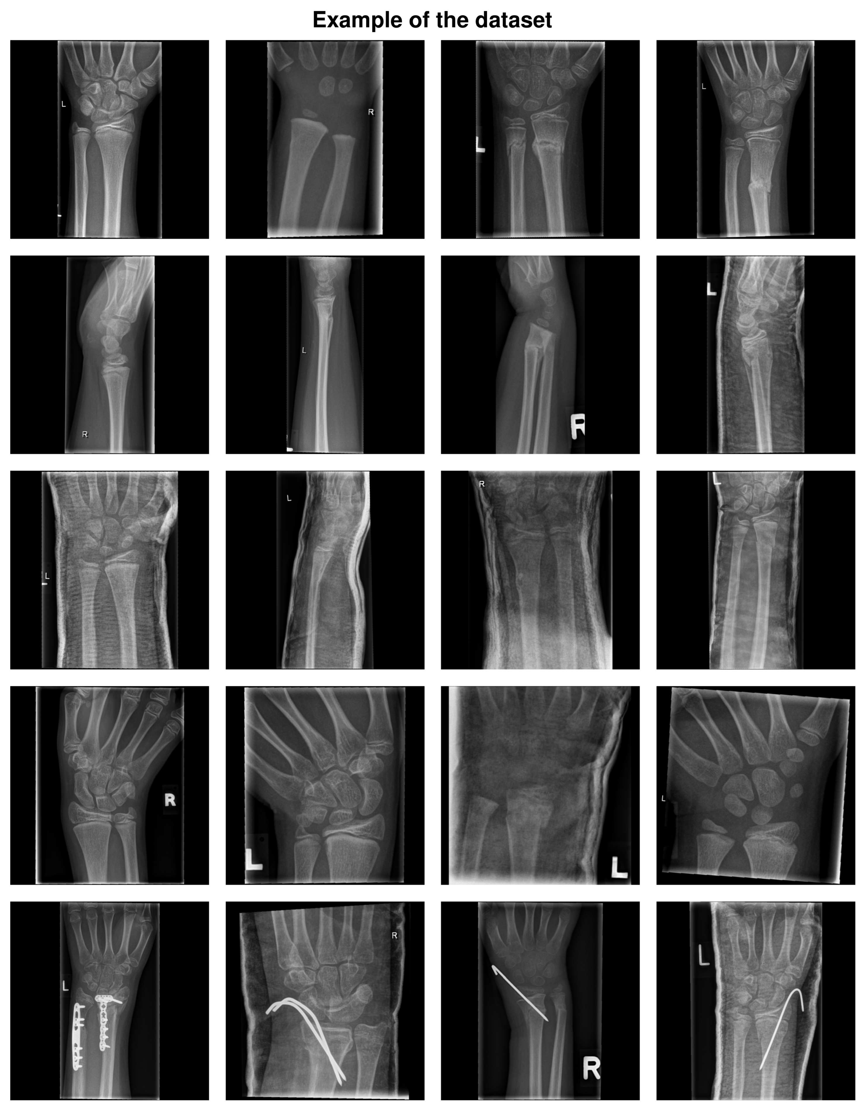
• We hypothesise that fractures in the near vicinity of the wrist in paediatric X-ray images can be identified and localised efficiently using the YOLOv4 model proposed by Bochkovskiy et al. [15] (an object detection model). We test our hypothesis on a comprehensive expert-annotated paediatric wrist X-ray dataset. Paediatric X-ray images, compared to adult images, are more versatile in terms of injuries, possible diseases, and fracture shapes because of children’s bone growth and organ formation.
• To prove the excellence of the utilised method, we compare it against the current state-of-the-art method for fracture detection proposed by Lindsey et al. [11].
• We compare the results obtained by the trained model with the experts, getting an insight into how well the model performs compared to radiologists—on the same dataset.
• Along the same lines, we investigate radiologists’ performance while they are aided by our model, compared to their performance while they work unaided by it.

The novelty of our paper can be summarised as follows. We found that the YOLOv4-based approach can outperform radiologists and improve the accuracy of their predictions. We also found that the object detection approach is a better approach for fracture detection than the current state-of-the-art U-net-based segmentation approach. We draw our conclusions from experiments conducted on a complex real-world dataset of paediatric wrist fracture X-rays. To the best of our knowledge, this is the first application that works on real-world X-rays obtained in the clinic—involving also casts, different projections, presence of metal, etc.—utilising a well-known robust object detection model. Furthermore, we set guidelines required to create a (paediatric) wrist fracture detection decision support system based on our observations.

2. Materials and Methods

The ethics committee of the Medical University of Graz (IRB00002556) approved the study protocol (No. EK 31-108 ex 18/19). Due to the retrospective data analysis, the committee waived the requirement for informed patient or legal representative consent. We performed all study-related methods in accordance with the Declaration of Helsinki and the relevant guidelines and regulations. Furthermore, the dataset can be made available upon reasonable request.

2.1. Dataset

The dataset used in the research had been acquired between 2008 and 2018 by the Division of Paediatric Radiology, Department of Radiology, Medical University of Graz, Austria. It consists of 19,700 8-bit paediatric wrist X-ray images from 10,150 unique studies of 5997 unique paediatric patients. The examinations had been annotated by various students and radiologists between 2018 and 2020 via the Supervisely (Deep Systems LLC, Moscow, Russia) online tool by placing bounding boxes around areas containing a fracture. Three certified paediatric reference radiologists validated all annotations. Bounding boxes were adapted and corrected until a consensus was reached. That being said, the fractures were not verified by inspecting other imaging modalities, such as MRI.

In

Table 1. Dataset attributes.

Attribute	Attributes’ Value
Gender	Male: 8074	Female: 11,626	NA
Age	Male: 11.50 ± 3.61	Female: 10.44 ± 3.56	All: 11.07 ± 3.63
Fracture	Zero: 7119	One: 8780	Multiple: 3801
Projection	AP: 9775	LAT: 9835	OBL: 90
Side	Left: 10,791	Right: 8909	NA
Cast	Present: 14,103	Not present: 5597	NA
Metal	Present: 686	Not present: 19,014	NA

, we present an overview of the dataset characteristics, depicting its complexity. Average age of the patients was $11.07\pm 3.63$ ($11.50\pm 3.61$ for 8074 male patients, and $11.07\pm 3.63$ for $11,626$ female patients). From the total number of X-ray images, 7119 did not contain fractures, 8780 had one fracture present, while 3801 had two or more fractures present. Furthermore, in Table 1, we present distributions of other features presented in the images, such as projection, side, presence of cast, and presence of metal. We should mention that 9573 studies ($94.3\%$) contained both anteroposterior and lateral projections. We did not exclude any type of image, making the utilised dataset challenging for modelling, yet realistic in common clinical practice. In the Appendix A Figure A1. we show a mosaic depicting the variety of the X-ray images in the dataset used.

From the available images in the dataset, we generated four randomly sampled disjoint subsets:

• Training dataset consisting of $15,600$ images.
• Validation dataset consisting of 1950 images, used for model selection (tuning hyperparameter values, such as learning rate or batch size).
• Test dataset #1, consisting of 1950 images, used for the final inspection of models’ generalisation properties.
• Test dataset #2, consisting of 200 images, used for expert evaluation. Of the 200 images, one half did not contain any fractures while the remaining images contained at least one fracture. This kind of selection was important to properly evaluate the models against radiologists.

To summarise, for model evaluation against the baseline method [11], we used the training, validation, and test (#1) data subset (19,500 images in total), while for the evaluation of the best performing model—with or against radiologists—we used the test subset (#2) of 200 images.

For image preprocessing, aligning images in such a manner that the fingers always pointed to the top image border, we followed the guidelines laid out in Lindsey et al. [11]. This orientation is present in multiple papers dealing with wrist fracture detection; however, it is not always emphasised. X-ray image alignment and orientation was conducted utilising XAOM [16]. The final image size was $960\times 960$ pixels (XAOM zero-pads images in both dimensions, as required). No denoising actions were taken because the images were of high quality, as is generally the case with X-ray images. To the best of our knowledge, the only publicly available dataset contains only 193 images of questionable quality with no information about annotations at all [17]. Therefore, we have conducted all training and testing of the models on our dataset.

2.2. Utilised Methods

In our study, we used the YOLOv4 model and compared it to the slightly adapted U-Net model proposed in Bochkovskiy et al. [15] and Lindsey et al. [11]. In the following subsections, we explain the motivation behind using these approaches, as well as the methods themselves.

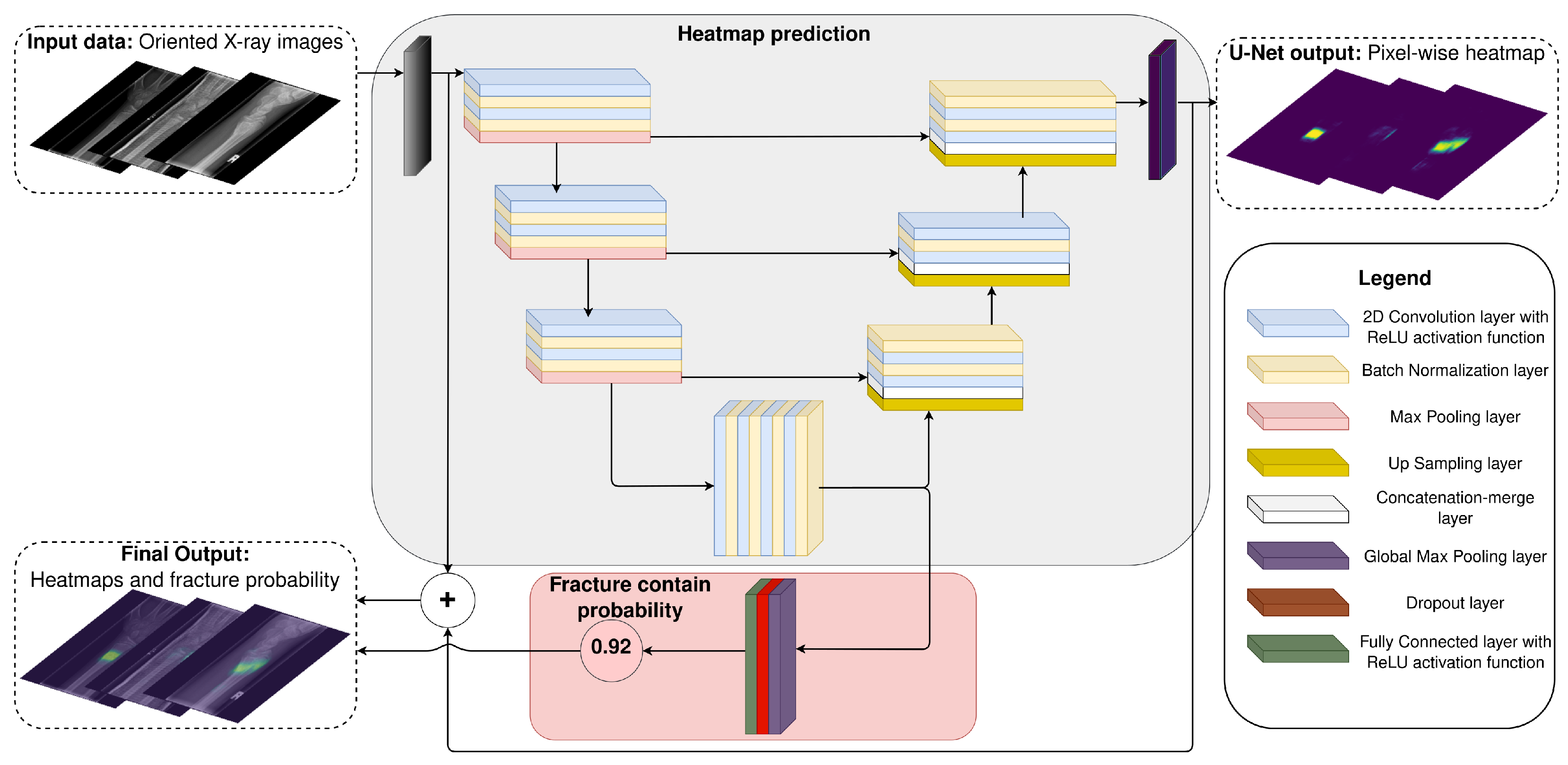
2.2.1. U-Net—A State-Of-The-Art Wrist Fracture Detection Method

The most relevant approach (current state-of-the-art) for wrist fracture detection is described in Lindsey et al. [11]. In their work, the authors proposed a novel method based on the U-net neural network (NN) model [18,19,20,21]. Because their dataset is not publicly available, we adjusted and trained their method on our dataset. The adjustments we made to the method did not impair the original model proposed in their work.

The U-Net model, as depicted in Figure 1, consists of two major parts:

(1)

The first part produces a pixel-wise heat map (mask) representing the probability for each pixel to belong to a fracture. This part is a U-net model with the same layer specification as described in the original paper (convolutional kernel size, padding, number of filters, etc.).

(2)

The second part calculates the probability that the input X-ray image contains a fracture. It consists of a global max pooling layer followed by a dropout layer with a dropout probability of $0.5$ (same as the original paper). Because there was no information concerning the fully connected layer, we set the number of neurons to 4096 with the ReLU activation function (inspired by the VGG19 model head [22])

To stabilise training, ensuring loss function convergence on our dataset, besides the originally proposed L2 regularisation ($\lambda ={10}^{-5}$), we applied ReLU activations after every convolutional layer (instead of every other convolutional layer, which was the case in the original paper). Moreover, after each convolutional layer, we added a batch normalisation layer that also helped with model convergence during training [23]. The output layers were the same as in the original paper (sigmoid activation function).

Due to our hardware limitations, the input size of the image was set to $512\times 512$ (instead of $1024\times 512$). The batch size was set to 8. The model was trained for 500 epochs with early stopping set to 6 epochs without improvement on the validation set. Loss function was the sum of two binary cross-entropy functions (heat map and fracture probability), and the optimiser was Adam with a learning rate $\alpha ={10}^{-4}$ [24]. Data preparation and augmentation were performed in the same way as in the original paper. Furthermore, in the original paper, the authors pretrained their U-net model using 100,855 X-ray images of 11 different body parts. We also pretrained the U-Net model on 84,084 X-ray images containing 21 different body regions (regions being uniformly distributed).

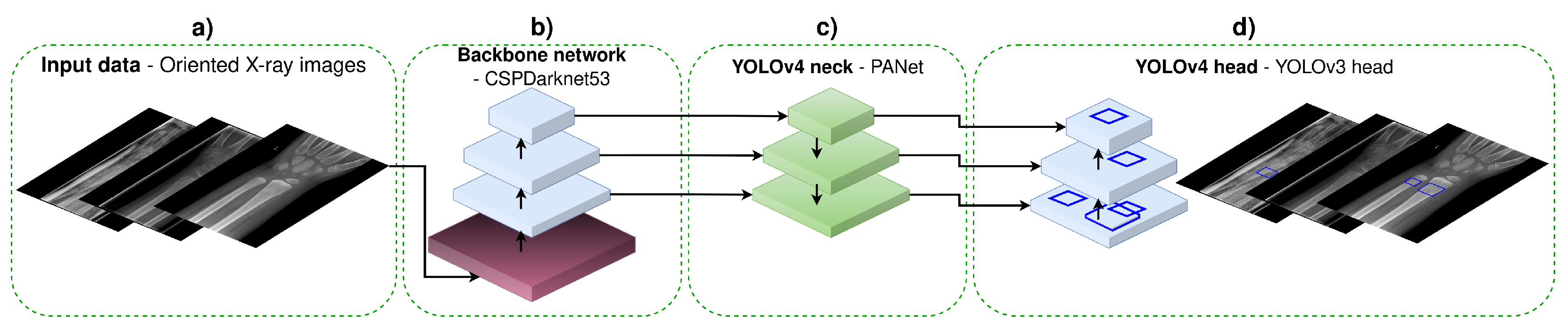
2.2.2. You-Only-Look-Once YOLOv4

YOLOv4 model is the current state-of-the-art approach for object detection. YOLOv4 started as YOLOv1 [25] in 2015 and since then experienced several enhancements in topology and exploited numerous concepts [15]. Its name is an acronym of You-Only-Look-Once, which indicates it as a one-stage detector, and not two-stage—such as region proposal convolutional neural network (CNN) [26,27,28]. Bochkovskiy et al. [15] conducted an extensive—time and resource consuming— comparison of YOLOv4 with different state-of-the-art models for object detection and did an extensive search for the best topology of their proposed method. Therefore, as the starting point of our research, we considered their findings and used the model that achieved the best results in their paper. Furthermore, numerous papers are comparing YOLOv4 to other available object detection methods where YOLOv4 attains similar or better performance [29,30,31,32]. This motivated us to use the YOLOv4 model in our research. YOLOv4 consists of four main parts, depicted in Figure 2:

• Input data—this step includes augmentation and preprocessing of the input data (XAOM with image scaling to $512\times 512$, and $608\times 608$ pixels). In our research, we have utilised the same data augmentation methods (bag of freebies, mosaic augmentation, etc.), and image sizes that were proposed in the original YOLOv4 paper [15].
• Backbone network is a feature extractor CNN. In the original YOLOv4 paper, the authors compared several backbone CNNs, with CSPDarknet53 being the best-performing one [33]. Hence, in our work, we have utilised the same CNN model accompanied with the proposed enhancements (known as the bag of specials).
• YOLOv4 neck is used for feature aggregation. In the original paper, the authors discussed several model architectures for feature aggregation and decided to utilise PANet for aggregating features [34]. In our research, we followed the same intuition and utilised PANet as well.
• YOLOv4 head has the role of a detector, producing a vector representing objects (in our case, fractures). Each object is defined with an anchor (the coordinates of the predicted bounding box: center, height, width) and class probability. The utilised head was the same as in the original paper [35].

Class prediction accuracy and estimated bounding box area (intersect-over-union score) can be increased by setting up the initial estimations of the anchor’s sizes. The anchors’ size estimations are completed by running the k-means clustering algorithm over the training dataset with the number of clusters set to nine [36]. Therefore, in total, we trained and tested four YOLOv4 models for fracture detection:

• YOLO 512 model having the input image size set to $512\times 512$ and original anchor sizes: $(12,16)$, $(19,36)$, $(40,28)$, $(36,75)$, $(76,55)$, $(72,146)$, $(142,110)$, $(192,243)$, $(459,401)$.
• YOLO 512 Anchors model having the input image size set to $512\times 512$ and estimated anchor sizes: $(23,22)$, $(44,27)$, $(35,40)$, $(73,31)$, $(55,41)$, $(61,62)$, $(84,47)$, $(101,67)$, $(92,115)$.
• YOLO 608 model having the input image size set to $608\times 608$ and original anchor sizes: $(12,16)$, $(19,36)$, $(40,28)$, $(36,75)$, $(76,55)$, $(72,146)$, $(142,110)$, $(192,243)$, $(459,401)$.
• YOLO 608 Anchors model having the input image size set to $608\times 608$ and estimated anchor sizes: $(40,41)$, $(70,51)$, $(109,58)$, $(82,82)$, $(157,70)$, $(122,94)$, $(114,155)$, $(176,111)$, $(206,176)$.

All other hyperparameters were the same as proposed in the original paper except for the optimiser learning rate $\alpha$ that was empirically defined based on the values reported in the original paper. The hyperparameters are as follows: optimiser is a stochastic gradient descent (SGD) (learning rate $\alpha =0.0013$ was chosen between values proposed in the original paper: $0.01$ and $0.00261$, and is multiplied with a factor $0.1$ at ≈80 epochs, momentum $0.949$, decay $0.0005$, burn-in for $1.000$ steps), batch size is set to 64 with 32 subdivisions, and regularisation method was dropBlock with drop probability of $0.1$. PANet (SPP module) used max-pooling layers with kernel size $k\times k$, where k = $1,5,9,13$. The config files and trained models’ weights are available on the following DOI:doi:10.6084/m9.figshare.16963426 (accessed on 11 August 2022). Moreover, all tested models were trained until there was no significant improvement in the accuracy on the validation set. Usually, this occurred after ≈100–150 epochs (around three days of parallel training on three NVIDIA GeForce RTX 2080 Ti GPUs per model). While this research was conducted, YOLOv4 was the most recent version. Later on, we decided to release a complex paediatric wrist dataset based on the one that we used in this research [37]. With the knowledge of YOLOv4 performance, we decided to set a baseline result on the released dataset with the YOLOv5 [38]. YOLOv5 (at that moment, the most recent version of YOLO) obtained comparable results to the YOLOv4 utilised in this research. This means that newer versions of the YOLO algorithm could perform as well or even better than the YOLOv4, which was the state-of-the-art YOLO model when this research was conducted.

2.2.3. Methods Evaluation

To evaluate model performance fairly, we utilised three different evaluations on the test set #1 (having 1950 images):

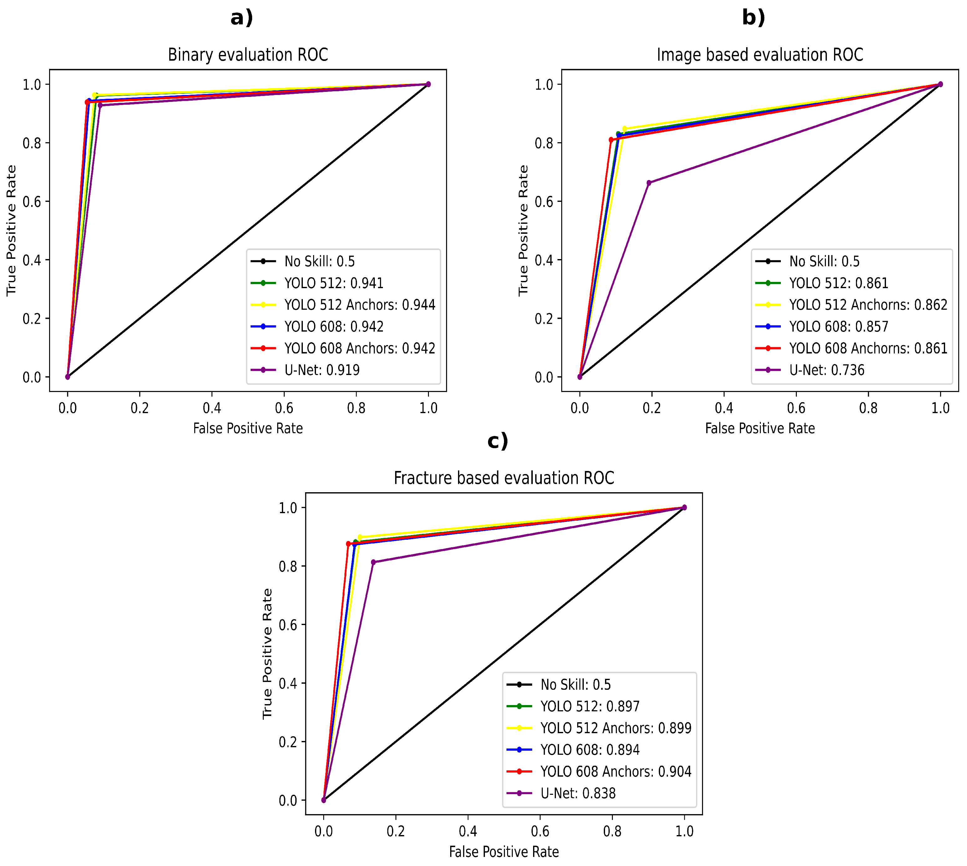
• The first evaluation benchmark involves a binary (yes/no answer) fracture presence classification task. Hence, we named it binary evaluation. This evaluation is designed according to work presented in Lindsey et al. [11]. Because the YOLOv4 method outputs a probability for each detected fracture, we would take the highest detected fracture probability in an image as the outputted value. For the U-Net model, we would simply take its second part/branch output. To obtain the models’ best performance, we used the fracture contain probability threshold $\gamma$—if the probability was below the set threshold value, there was no fracture presented in the image.
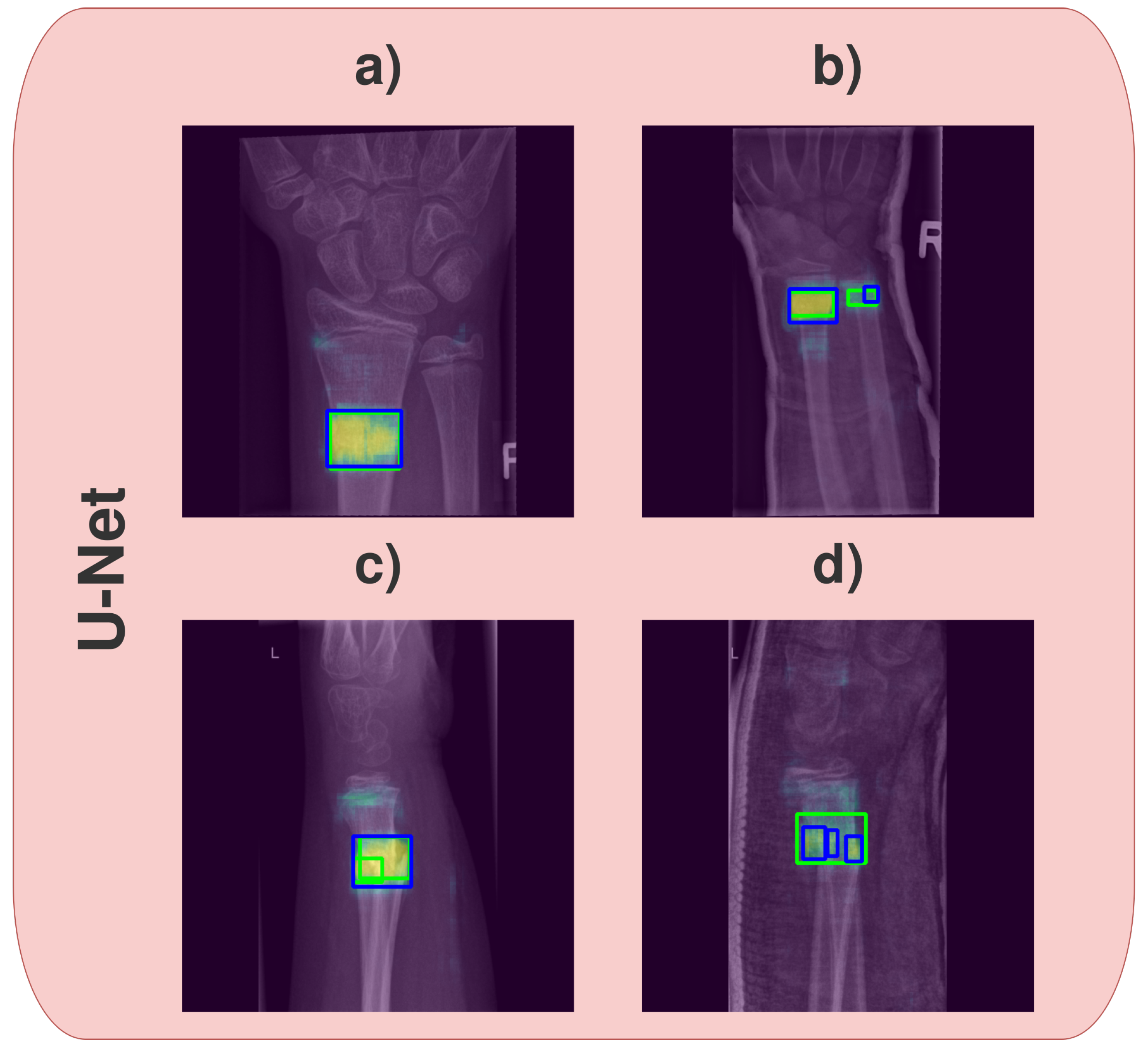
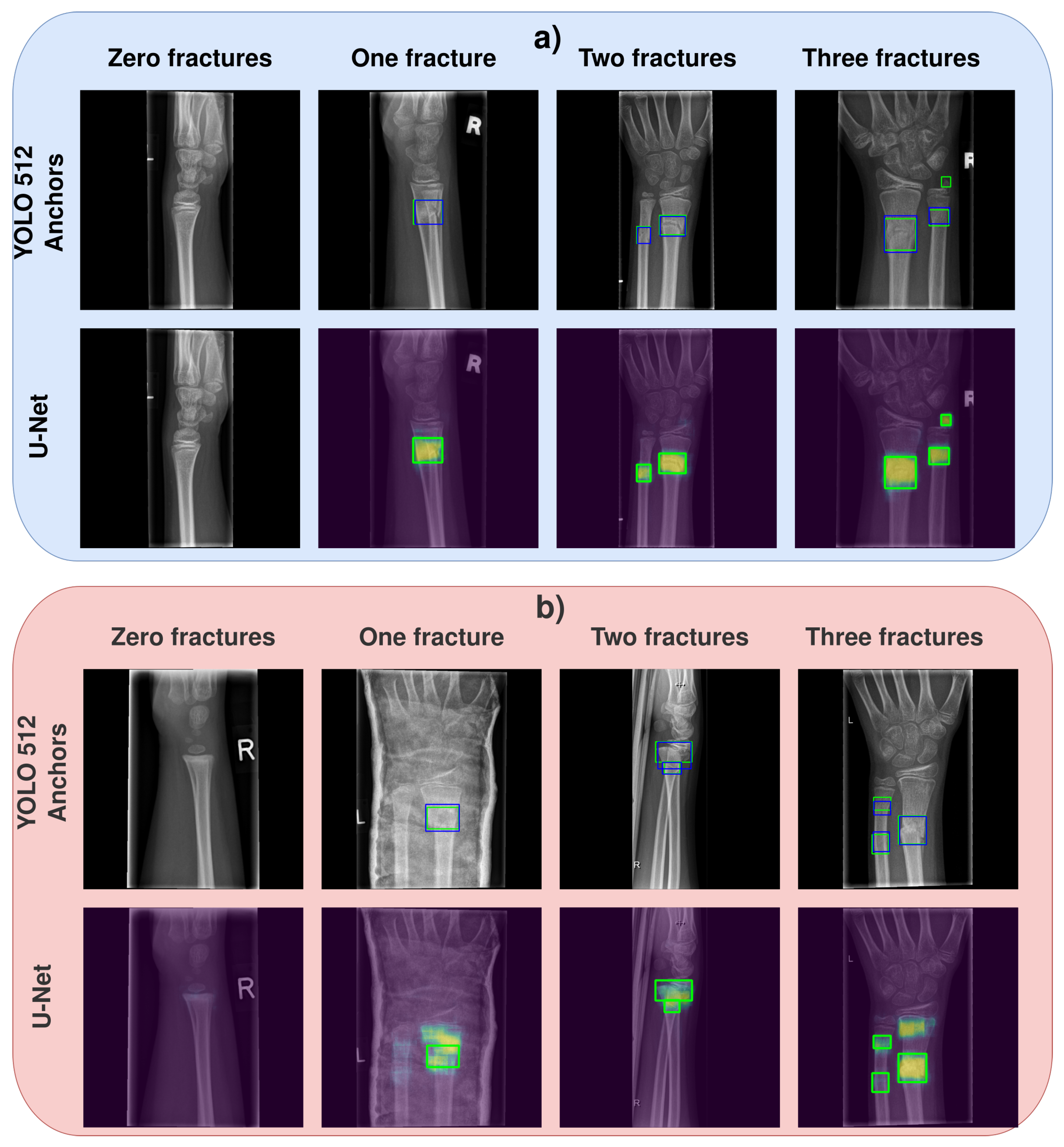
• The second evaluation benchmark we named image-based evaluation. In this test, we count the number of detected fractures in the image. To elaborate, in image-based evaluation, a true positive means that the number of detected fractures by the model is the same as the actual number of fractures in the image. If the model detects more than the actual number of fractures, it is a false positive. On the other hand, if it detects fewer fractures than the actual number of fractures, it is a false negative (if the image does not contain any fractures and models predict zero fractures, it is a true negative). For the YOLOv4 method, the image-based evaluation was simple because the method already outputs bounding boxes, including the probabilities that each bounding box contains a fracture. For the U-Net model, we had to develop an algorithm for bounding box (region) extraction. The algorithm first set heat maps to black-blank images (no fracture, 0 probability) if the second part of the U-Net model (fracture-contain probability) is lower than the experimentally defined threshold value $\gamma$. Second, the remaining heat map representing the fracture’s pixel-wise probability is binarised using another experimentally defined threshold value (heat map probability $\theta$). Last, we estimate the minimum bounding boxes of the fractures based on the remaining regions of white pixels, utilising the convex-hull algorithm [39]. Each bounding box represents one fracture, which allowed us to count the fractures by simply counting the bounding boxes. The image-based evaluation worked for the YOLOv4 model, but it did not evaluate the U-Net model properly due to the issues illustrated in Figure 3. Namely, after applying both threshold values ($\gamma$ and $\theta$), one heat map would sometimes be split into two separate bounding boxes. The opposite case is also present where, based on the heat map, only one bounding box is detected, while multiple fractures are present in close proximity to one another. Another issue is that the bounding box (after applying the threshold values) would sometimes be rather small compared to the whole heat map region, although the whole heat map perfectly fits the true bounding box of a fracture. Therefore, the image-based evaluation serves the purpose of giving us a rough estimation of models’ performance during training. For the true model performance, we propose the third evaluation.
• Third, and the most rigorous evaluation benchmark is the fracture-based evaluation. In this evaluation, we went manually through each image and evaluated every fracture separately, which means that if the image contained two fractures, we would have two evaluations for that particular image (one evaluation for each fracture). The match was positive if the IoU score of the predicted bounding box by the YOLOv4 model and the true fracture bounding box was $0.5$ or higher, or if the heat map generated by the U-Net model was over $50\%$ overlapped with the expected fracture region (the heat map was not smeared by more than $50\%$ with respect to the bounding box). For this evaluation, we also used the threshold $\gamma$; any fracture with a probability less than the set threshold value was not considered.

Both threshold values ($\gamma$ and $\theta$) were experimentally determined using the validation dataset. A grid-search algorithm determined the optimal values over the hyperparameter space, ranging from $5\%$ to $100\%$ (step size $2.5\%$). The best performing threshold-value combination was the one attaining the highest F1-score and accuracy (the two metrics that we considered to be the most important). Because of the vast hyperparameter space, we utilised the same threshold values used for image-based evaluation for the fracture-based evaluation. Namely, to check each $\gamma /\theta$ value combination for fracture-based evaluation on the validation set, we would need to manually score 1950 images—for every model, for each threshold combination – making this effort unfeasible. Moreover, because the models were developed specifically for wrist fracture detection, we did not evaluate them on other-domain datasets.

For the radiologists’ evaluation and comparison, we have utilised the test dataset #2, consisting of 200 images. We wanted to perform the following two evaluations:

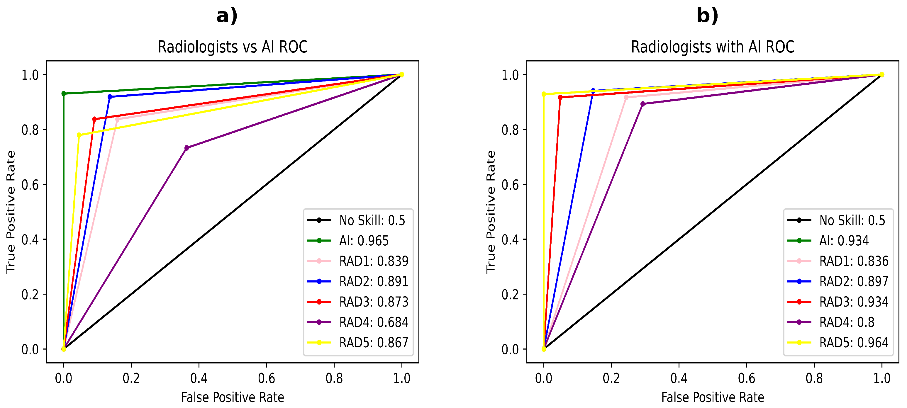
• The first evaluation is radiologist-versus-AI. This evaluation is similar to the fracture-based evaluation. The radiologists had the same task as the AI method: to draw bounding boxes around the fractures. Here, we compare the performance of five radiologists, who separately took the test against the best performing AI model, according to the prior evaluation tests.
• The second evaluation is radiologist-with-AI, where the radiologists are given the output of the AI (AI-predicted bounding boxes), and allow the radiologists to agree or disagree with the AI prediction. A radiologist can agree with the AI prediction or change it; however, once the radiologist makes the decision, it cannot be reversed. In the images not having any fractures, the assistance would simply be given such that the AI thinks there is no fracture present (just to make it clearer to the radiologists).

After obtaining the best-performing model, we ran it on 200 images (test set #2). Based on the obtained model predictions for every image, we sampled two disjoint subsets—one for each evaluation. The disjoint subsets (each having 100 images) were sampled so that the model retained approximately similar performance (F1-score and accuracy) on both. The sampling process was done without human interaction, so there was no bias present. We wrote an algorithm that selected an equal number of false positive (FP), true positive (TP), false negative (FN), and true negative (TN) classified images and uniformly divided them into two subsets. Moreover, our sampling algorithm did some additional balancing, such that, in the case of an odd number of images in one category (e.g., TP), it considered which subset had more images and simply added the surplus to the other one. Therefore, although the images were not the same in both evaluation datasets, the predictive model used for the AI-method tests had similar performance on both of them, making the results obtained by the radiologists on the evaluations comparable. Furthermore, we randomly shuffled each of the subsets for every radiologist. Therefore, there was not any bias present during the evaluation. Radiologists in training and board-certified radiologists underwent the tests. Experiences in musculoskeletal radiography were 8 years for RAD1, 6 years for RAD2, 3 years for RAD3, 5 years for RAD4, and 4 years for RAD5. By performing these tests, we mimicked the usual practice of the radiologists in the real-life clinical environments for wrist fracture detection.

The metrics used during the evaluations on the test set #2 are precision, recall, F1-score, accuracy, and area under the receiver operating characteristic curve (AUC-ROC). To measure the significance of the obtained results, we have performed McNemars’ significance test and the two-tailed T-test [40,41]. The statistical analysis was performed using the SPSS Statistics Version 21 (IBM Corp., Armonk, NY, USA) software. We regarded the p-value $p<0.05$ as statistically significant.

Figure 4 depicts a summary of the model evaluation process conducted in this research.

3. Results and Discussion

3.1. Models Evaluation Results

This section discusses the results of the YOLOv4 and the U-Net models, and the benefits and shortcomings of their respective output marks of the fractures.

3.1.1. Quantitative Analysis of the Models’ Result

In

Table 2. Binary evaluation of the models on test set #1.

Model Name	Fracture Contain Probability $\mathit{\gamma }$	Precision	Recall	F1-Score	Accuracy
YOLO 512	20.00%	0.94658	0.94667	0.94661	0.94667
YOLO 512 Anchors	25.00%	0.94969	0.94974	0.94971	0.94974
YOLO 608	22.50%	0.94311	0.94205	0.94233	0.94205
YOLO 608 Anchors	22.50%	0.94264	0.94103	0.94139	0.94103
U-Net	72.50%	0.92268	0.92154	0.92189	0.92154

* Bolded values represent the best obtained scores for each metric.

,

Table 3. Image-based evaluation of the models on test set #1.

Model Name	Fracture Contain Probability $\mathit{\gamma }$	Heat Map Probability $\mathit{\theta }$	Precision	Recall	F1-Score	Accuracy
YOLO 512	37.50%	/	0.86455	0.85385	0.85556	0.85385
YOLO 512 Anchors	37.50%	/	0.86470	0.85846	0.85973	0.85846
YOLO 608	35.00%	/	0.86063	0.84923	0.85103	0.84923
YOLO 608 Anchors	32.50%	/	0.86570	0.84821	0.85051	0.84821
U-Net	2.50%	65.00%	0.74644	0.72359	0.72516	0.72359

* Bolded values represent the best obtained scores for each metric, “/” represents the un-availability of the parameter for a given method.

and

Table 4. Fracture-based evaluation of the models on test set #1.

Model Name	Fracture Contain Probability $\mathit{\gamma }$	Precision	Recall	F1-Score	Accuracy
512	37.50%	0.89997	0.89144	0.89327	0.89144
YOLO 512 Anchors	37.50%	0.90369	0.89871	0.89997	0.89871
YOLO 608	35.00%	0.89718	0.88701	0.88907	0.88701
YOLO 608 Anchors	32.50%	0.90502	0.89387	0.89592	0.89387
U-Net	2.50%	0.84805	0.82889	0.83292	0.82889

* Bolded values represents the best obtained scores for each metric.

, we present the results for binary, image-based, and fracture-based model evaluation benchmarks, respectively (best results are emphasised). The tables also contain the values of utilised thresholds, $\gamma$ and $\theta$, for each model. The thresholds were set according to their best-achieved results on the validation dataset, as described in Section 2.

In all three evaluations, the YOLO 512 Anchors model attained the best results while the U-Net model was constantly the worst. Precision was the only metric where the YOLO 512 Anchors model was not performing best in all three evaluations. Namely, for image-based (Table 3) and fracture-based (Table 4) evaluation, the YOLO 608 Anchors model attained the best precision score. For binary evaluation (Table 2), the best precision was attained by the YOLO 512 Anchors models.

In a–c of Figure 5, we present ROC curves and AUC-ROC values of each tested model for every evaluation. The results suggest that the YOLOv4 models outperformed the U-Net model in every evaluation. For binary evaluation, the average ROC-AUC values of YOLOv4 models were $0.942\pm 0.001$, while the U-Net models’ AUC-ROC value was $0.919$. The same trend is followed by image-based evaluation (YOLOv4 models AUC-ROC value $0.860\pm 0.002$ versus U-Net model AUC-ROC value $0.736$) and fracture-based evaluation (YOLOv4 models AUC-ROC value $0.899\pm 0.004$ U-Net model AUC-ROC of $0.838$).

To statistically confirm that YOLOv4 models perform better than the U-Net model, we conducted McNemars’ test. The test has shown a significant difference at level $p<0.05$ between all models based on the YOLOv4 model and the U-Net model (calculated values for each of the three evaluations are presented in

Table A1. McNemars’ test for binary evaluation of the methods. Bolded values represents statistical significance at the $p<0.01$ level.

	YOLO 512	YOLO 512 Anchors	YOLO 608	YOLO 608 Anchors	U-Net
YOLO 512	1	0.51184	0.32108	0.23510	2.99 × 10${}^{-5}$
YOLO 512 Anchors	0.51184	1	0.08168	0.05681	5.93 × 10${}^{-7}$
YOLO 608	0.32108	0.08168	1	0.89568	0.00063
YOLO 608 Anchors	0.23510	0.05681	0.89568	1	0.00167
U-Net	2.99 × 10${}^{-5}$	5.93 × 10${}^{-7}$	0.00063	0.00167	1

,

Table A2. McNemars’ test for image-based evaluation of the methods. Bolded values represent statistical significance at the $p<0.01$ level.

	YOLO 512	YOLO 512 Anchors	YOLO 608	YOLO 608 Anchors	U-Net
YOLO 512	1	0.48472	0.51516	0.39979	1.07 × 10${}^{-39}$
YOLO 512 Anchors	0.48472	1	0.16207	0.11554	1.65 × 10${}^{-40}$
YOLO 608	0.51516	0.16207	1	0.93171	6.42 × 10${}^{-36}$
YOLO 608 Anchors	0.39979	0.11554	0.93171	1	6.40 × 10${}^{-37}$
U-Net	1.07 × 10${}^{-39}$	1.65 × 10${}^{-40}$	6.42 × 10${}^{-36}$	6.40 × 10${}^{-37}$	1

and

Table A3. McNemars’ test for fracture-based evaluation of the methods. Bolded values represent statistical significance at the $p<0.01$ level.

	YOLO 512	YOLO 512 Anchors	YOLO 608	YOLO 608 Anchors	U-Net
YOLO 512	1	0.14166	0.42784	0.68905	1.01 × 10${}^{-17}$
YOLO 512 Anchors	0.14166	1	0.02420	0.37546	2.11 × 10${}^{-21}$
YOLO 608	0.42784	0.02420	1	0.17453	8.83 × 10${}^{-15}$
YOLO 608 Anchors	0.68905	0.37546	0.17453	1	2.72 × 10${}^{-19}$
U-Net	1.01 × 10${}^{-17}$	2.11 × 10${}^{-21}$	8.83 × 10${}^{-15}$	2.72 × 10${}^{-19}$	1

of the Appendix A). However, among the YOLOv4-based models, we observed no significant difference.

3.1.2. Analysis of Models’ Output Labels

In Figure 6a, we display the results of the YOLO 512 Anchors model and the U-Net model on images containing zero, one, two, or three fractures. In Figure 6b, we illustrate some of the difficulties that we encountered during fracture segmentation (which YOLOv4 based methods did not have). Namely, in the case with zero fractures, the U-Net model predicted that the image contains a fracture ($\gamma \sim 90\%$); however, a heat map did not show any fracture. In that case, we would say there is no fracture if we are performing the fracture-based evaluation. However, this decision is debatable. Furthermore, in the image containing only one fracture (Figure 6b), the fracture heat map is smeared for the U-net model, making the fracture more opaque. This is not an error, namely the fracture is correctly marked, only it is more challenging to determine where the fracture is in comparison with the boundary boxes predicted by the YOLOv4-based models. In the image containing two fractures (Figure 6b), the real shortcoming of the U-Net model is shown. Namely, based on the heat map, when the two fractures are nearby, it is nearly impossible to distinguish if there is only one big fracture or two smaller fractures present instead. By using a suitable threshold $\theta$, splitting the one big heat map into two smaller heat maps would be possible. However, in the case that the image contains one big fracture, the selected threshold would create false positives. On the other hand, we found that YOLOv4-based models do not suffer from these issues because they inherently treat each fracture as a separate object. Moreover, from the clinical point of view, it is important to mark each fracture because, during fracture reporting, each fracture must be acknowledged. Finally, in Figure 6b, we present an image containing three fractures, where one fracture is erroneously marked. Although we present this for the U-Net model, it applies to the YOLOv4-based models as well. The number of detected fractures is correct; however, one or more fractures are erroneously marked. This issue is crucial because it shows the biggest drawback of the proposed models: the experts must check the results, meaning that the models can not operate standalone and should be used only as assisting tools.

3.1.3. Summary of Models Comparison

To summarise, all three evaluation benchmarks had the same outcome: from the binary evaluation (that can be seen as classification) that does not explain the decisions to the in-depth manual analysis of fracture presence where each fracture is predicted using a boundary box, YOLOv4-based models outperformed the U-Net model. Furthermore, we should emphasise that the heat map is suffering from several problems not afflicting bounding boxes. For example, treating fractures as an object represented by the bounding box yielded more interpretive and human-friendly results. Although there was no significant difference between the respective YOLOv4-based models, YOLO 512 Anchors model consistently attained top recall, F1-score, and accuracy, in all tests. Therefore, we decided to use the YOLO 512 Anchors model in the following experiments.

3.2. Radiologist and AI Comparison

In

Table 5. RAD vs. AI—fracture-based evaluation on test set #2.

Test Subject	Precision	Recall	F1-Score	Accuracy
YOLO 512 Anchors	0.95938	0.95385	0.95449	0.95385
RAD1	0.84847	0.83846	0.84099	0.83846
RAD2	0.90065	0.9	0.90027	0.9
RAD3	0.87743	0.86154	0.86433	0.86154
RAD4	0.71338	0.7	0.70469	0.7
RAD5	0.87540	0.83846	0.84268	0.83846

* Bolded values represent the best obtained scores for each metric.

, we present the results of AI (YOLO 512 Anchors model) against the radiologists on the test data #2 subset of 100 images. It can be noticed that AI outperformed the radiologists in all metrics. The same trend can also be observed in ROC curves and AUC-ROC values presented in Figure 7. AI attained the AUC-ROC value of $0.965$, while the averaged radiologist’s AUC-ROC was $0.831\pm 0.075$. Furthermore, McNemars’ test (presented in Table A3 of the Appendix A) suggests that the AI performs significantly better than the radiologists RAD1, RAD3, RAD4, and RAD5 under confidence level $p<0.05$; however, it does not perform significantly better than RAD2 at the same level ($p=0.0654$). Moreover, in Figure 8 we depict several images with labels from the radiologists and AI. As it can be noticed, the AI labels (green colour) are precise and consistent around the white area that represents ground truth, while the radiologists’ labels vary. Furthermore, if somebody makes a mistake, it is manifested as not recognising a fracture at all (rather than wrongly labelling it). Based on the labels area, we can conclude that the CAD system built on top of the AI will mark a similar area around the fracture as it would be the case if a radiologist were doing it. However, the CAD system will always be consistent in its fracture area mark, which is not the case with radiologists.

In

Table 6. Radiologist with AI—fracture-based evaluation on test set #2.

Test Subject	Precision	Recall	F1-Score	Accuracy
YOLO 512 Anchors	0.93307	0.928	0.92896	0.928
RAD1	0.86233	0.864	0.86261	0.864
RAD2	0.91156	0.912	0.91171	0.912
RAD3	0.93307	0.928	0.92896	0.928
RAD4	0.82962	0.832	0.83028	0.832
RAD5	0.95812	0.952	0.95274	0.952

, we present the results of radiologists’ performance aided by the AI (the AI decision was present in the images that the radiologists needed to mark). Two-tailed independent sample t-test confirms that there is no statistical difference of the AI performance on the test used in radiologist versus AI evaluation and radiologist with AI evaluation ($t=0.87476$; $p=0.38254$). Detailed results are presented in the Appendix A 

Table A5. Two-tailed independent t-test results between radiologists with and without AI help. Bolded values represent statistical significance at the $p<0.05$ level ($d{f}_1=129,$ $d{f}_2=124$).

	AI	RAD1	RAD2	RAD3	RAD4	RAD5
t	0.87476	−0.57061	−0.32685	−1.72765	−2.50488	−2.98537
p	0.38254	0.56877	0.74405	0.08527	0.01288	0.00311

.

This suggests that the data from test set #2 was sampled evenly, and there is no bias present favouring the AI. The result has shown that all radiologist increased their performance when aided by the AI:

• RAD1 F1-score increased from $0.84099$ to $0.86261$;
• RAD2 F1-score increased from $0.90027$ to $0.91171$;
• RAD3 F1-score increased from $0.86433$ to $0.92896$;
• RAD4 F1-score increased from $0.70469$ to $0.83028$;
• RAD5 F1-score increased from $0.84268$ to $0.95274$.

However, by performing two-tailed independent sample t-tests, the significant difference in performance was detected for RAD4 and RAD5 at significance level $p<0.05$. For RAD3, there was an improvement at significance level $p<0.10$ (the exact p-values and t-values are presented in the Table A5). For RAD1 and RAD2, we noticed no statistically significant improvement. We can conclude that the proposed AI method can improve a radiologist’s performance (which happened in three cases), or serve as support in decision making (for the two radiologists that did not have a significant statistical improvement). The improvement can also be noticed in ROC curves and AUC-ROC values presented in Figure 7b, which are following the same trend as the F1-score and the accuracy values.

3.3. Fracture Detection Problem and Related Work

A literature overview of wrist fracture detection yielded many exciting research approaches. To properly evaluate them and choose the most important work to compare the YOLOv4-based model with, we took into account the key features laid out in

Table 7. Overview of related work with descriptive atributes.

Paper	Data	Models	Type of Fracture Recognition	Result	Comparison with Experts
Ours	Projections: AP, LAT, Oblique Training: 15,600 images Test: Test #1: 1950 images, Test #2: 2 × 100 images	YOLOv4 based models	Fracture detection	AUC-ROC: Test #1 0.899 F1-Score: Test #1 0.89997 AUC-ROC: Test #2 0.899 F1-Score: Test #2 0.95449	Model outperformed radiologists and enhanced their performance.
Raisuddin et al. [6]	Projections: AP, LAT Training: 3873 images Test: Test1 414 images, Test2 210 images	ROI localisation block combined with SeresNet50 fracture classificator. Heat map with GradCAM method	Classification with heat map segmentation	AUC ROC: Test1 0.99 (0.98–0.99) F1-Score: Test1 0.95 (0.92–0.97) AUC ROC: Test2 0.84 (0.72–0.93) F1-Score: Test2 0.63 (0.44–0.80)	Model outperformed physicians (both tests) and was better than the radiologists on the Test2
Blüthgen et al. [10]	Projections: AP, LAT Training: 524 images Test: 100 images (internal), 200 images (external)	Deep Learning System(DLS), Two not defined models	Classification based on the heat map overlap	AUC ROC: 0.96 (0.87–1), 0.89 (0.81–0.94) Fracture localization: 94%, 83%	Radiologist were comparable Or better than the DLS
Gan et al. [9]	Projections: AP Training: 2040 images Test: 300 images	Faster R-CNN for fracture extraction, Inception-v4 for ROI classification	Classification of the detected fractures	AUC ROC:0.96 (0.94–0.99) IOU: 0.87 (0.86–0.87)	Model results were comparable with orthopedics, and better than radiologists
Thian et al. [7]	Projections: AP, LAT Training: 6515 AP images, 6537 LAT images Test: 525 AP images, 525 LAT images	Two Faster R-CNN models: One for each projection	Fracture detection	AUC ROC: AP 0.918 (0.894–0.941), AUC ROC: LAT 0.933 (0.912, 0.954)	None
Yahalomi et al. [8]	Projections: AP Training: 120 images (Augmented to 4476) Test: 1312 images	Faster R-CNN: Pretrained on Image-net	Fracture detection	Accuracy: 96% MAP: 0.866	None
Kim and MacKinnon [5]	Projections: LAT Training: 1389 (Augmented to 11,112) Test: 100 images	Inception-v3	Classification	AUC ROC: 0.954	None
Lindsey et al. [11]	Projections AP, LAT Training: 31,490 images Test: Test1: 3500 images, Test2: 1400 images	Modified U-Net	Classification with heat map segmentation	AUC ROC: Test1 0.967 (0.960–0.973) AUC ROC: Test2 0.975 (0.965–0.0.982)	U-net model enhanced radiologists performance.
Olczak et al. [4]	Projections: AP, LAT, Oblique Training: 256,458 images (wrist, hand, ankle) Test: 400 images	VGG16	Classification	Accuracy: 83%	Model results were comparable With orthopaedics (∼82%)

. The key features are as follows: (1) Data—amount and variety of data used in the research; (2) Models—machine learning model type used in the approach; (3) Type of fracture recognition—type of task: classification, detection, or fracture segmentation; (4) Result—reported result in terms of model accuracy, and; (5) Comparison with experts—test of the proposed model against the experts.

The first criterion we considered is the dataset utilised in the research. Increased levels of variety in the data (metal, cast, projections, etc.) and the number of data instances cause the model trained on that data to be more robust [42,43]. Having this in mind, research presented by Gan et al. [9], Thian et al. [7], Yahalomi et al. [8], and Kim and MacKinnon [5] focuses only on one projection (either AP or LAT) and is therefore less suitable for applied medical usage. The second important data descriptor is the number of data instances (images) used for model training/testing. Researchers Olczak et al. [4], Lindsey et al. [11], and Thian et al. [7] used over 5000 images for model training which, in our opinion, should be sufficient for including all different types of fractures. All other researches utilised less than 5000 images, risking a smaller variety of fractures. For the model’s evaluation, the work presented by Blüthgen et al. [10], Yahalomi et al. [8], and Kim and MacKinnon [5] used under 300 images in the test set. In our opinion, a relatively small number of X-ray images can cause bias because it does not have a sufficient number of challenging—multiple fracture—cases. Namely, in real medical practice, detecting multiple fractures or tracing the fractures healing process under the cast are uncommon but important use cases. These use-cases may not be represented in a small sample of data, leading to model results unrepresentative of real-life usage. Finally, after carefully reviewing the descriptions of datasets in the mentioned works, we could not find any claim concerning using X-ray images containing metal or cast in them. Including this type of X-ray images leads to a more challenging distribution and, henceforth, to a more robust model trained learned from such data. Considering the mentioned criteria, Lindsey et al. [11] utilised the most complex and reliable dataset. We followed their example and utilised an even more demanding dataset because our dataset includes cast/metal and is built of paediatric wrist images, which are more demanding for analysis than adults’ fractures.

Utilised models in papers mainly govern the task being tackled. Therefore, the Models and Type of fracture recognition, as presented in Table 7 should be observed jointly. As mentioned before, based on the research presented in mentioned papers, three tasks can be distinguished: classification, detection, and fracture segmentation [44]. From the aspect of explainability, classification is the least useful to radiologists because it does not provide any insight into where the fracture could be, nor does it explain the model decision. Olczak et al. [4] utilised several popular neural network topologies (VGG16) to classify a wrist depicted on an X-ray image as fractured correctly, while Kim and MacKinnon [5] utilised Inceptionv3 for the same purpose. Raisuddin et al. [6] also performed a classification task using SeresNet50 with the GradCam method to provide explanations of the model’s decision. This brings us to the next key insight: the explainability of detected fractures (which the classification task lacks). The segmentation task is the most precise task of the fracture reporting, where each pixel gets categorised as part of a fracture. Therefore, research reported by Blüthgen et al. [10] and Lindsey et al. [11] is the most precise way of detecting fractures. However, their models, DLS and modified U-net (also presented in this paper), respectively, fail in the case when there are multiple fractures nearby (explained in Section 2.2.3). In the end, the most robust approach that still preserves enough explainability while being able to distinguish between multiple nearby fractures is the object detection approach. Therefore, Gan et al. [9], Thian et al. [7], and Yahalomi et al. [8] all used the Faster R-CNN model for fracture detection. The Faster R-CNN model is a two-stage detector that can be difficult to fine-tune. We wanted to prove that a single-stage detector such as YOLOv4 (which is easier to train) can obtain the same or even better accuracy. It is also necessary to mention that segmentation-based model outputs (heatmaps) can be easily transferred to bounding boxes by binarisation and estimating the minimum bounding rectangle. To conclude this deliberation, all research that is focused on fracture segmentation and detection is of interest. However, we found that the object detection approach can be more robust in case of multiple fractures. Furthermore, based on the reported results by related research and our own results, we did not find any direct bond between the results obtained by the models pre-trained on some data or when trained using randomly initialised weights. However, this could be a worthy topic for further investigation.

Speaking of Results, it is ungrateful to comment on them because all related work uses their own publicly unavailable datasets. To the best of our knowledge, there is no released code of their models which makes reproducing their results difficult (our code and models are available at DOI:doi:10.6084/m9.figshare.16963426) (accessed on 11 August 2022), consequently making a comparison based on reported results hard to discuss. Namely, all authors report remarkable results in terms of AUC-ROC, F1-score, and MaP (results are presented in Table 7). Yet, Lindsey et al. obtained the best results (if we disregard the classification tasks). However, it is not entirely fair to directly compare the results of specific metrics to each other. It is possible that a model that achieved better results on one dataset would perform poorly on another one. The one thing that can be observed is that the metrics mentioned are general approaches to validate models. One important subject that must not be neglected when validating the models that are supposed to help radiologists is the comparison with the radiologists themselves. The fact that the model helps or performs better than the radiologists on a given test is one way to be sure that the model is performing well. Of course, this claim stands as long as the test and metrics measuring performance are valid and fair.

Three works conducted by Thian et al. [7], Yahalomi et al. [8], and Kim and MacKinnon [5] did not compare their models with radiologists at all. On the other hand, Gan et al. [9], Olczak et al. [4], Blüthgen et al. [10], and Raisuddin et al. [6] proved that their models achieved similar or even better performance than the radiologists/orthopaedists. Lindsey et al. [11] have proven that clinicians can achieve better performance when aided by their proposed model. After careful analysis of the evaluation processes, we noticed that only Gan et al. [9] and Lindsey et al. [11] performed tests of statistical significance in their conducted experiments with radiologists, which makes their claims much stronger. We strongly advise using statistical tests to support the claims based on the obtained results, especially when the research revolves around enhancing experts’ performance. That being said, in our research, we followed the example of mentioned research that has conducted statistical tests and tailored our experiment similarly.

To summarise the above, we conclude with the following statements:

• Dataset must be representative: it must have a sufficient number of data instances where images include demanding cases with obstacles such as cast and metal and multiple fractures on different projections. This will increase the generalisation capacity of the trained model.
• The approach with the best trade-off between explainability and accuracy is the object detection approach. Namely, the segmentation approach fails when there are many fractures nearby.
• The results, unless they are presented on a public dataset, are not that informative. Although, metrics to be used are AUC-ROC, F1-Score, and possibly MaP.
• Comparison with radiologists is a necessity because that is the proof that the proposed model can be helpful in the clinic. When comparing the developed model with radiologists, statistical analysis is a must.

Therefore, we can say that Lindsey et al. [11], in their work, fulfilled the criteria mentioned above the best, and therefore, their work was selected as the appropriate state-of-the-art method. After comparison of our utilised method with the modified U-net method proposed by Lindsey et al., we can observe the following:

• The YOLOv4-based model outperformed the U-Net model on a complex dataset, utilising an in-depth, three-stage evaluation.
• The YOLOv4-based model outperformed most radiologists, same as the U-Net model.
• The YOLOv4 method enhanced the radiologists’ performance, similar to the U-Net paper research results.
• From an interpretability point of view, the YOLOv4 method more clearly depicts the fractures than the U-Net model.
• Both methods still need radiologist monitoring and can serve only as an assisting tool, not as a standalone application [45].

Finally, after careful inspection of mislabelled data, the problem of fractures that cannot be seen on X-ray but can be seen on MRI or CT still remains unsolved. The hypothesis is that the visibility of fractures in the plain X-ray data represented in 10–16 bits needs to be tested. Furthermore, we believe that merging the object detection approach with the segmentation approach is taking the best of both worlds. Thus, the idea is to either create a robust model assembly or develop an entirely new topology designed for this case [46]. Furthermore, one of the limitations of our (and other) research is the data that is collected from one hospital. This results in possible bias in the dataset that we might not be aware of (for instance, patient bias), which could, in the end, influence the trained model’s generalisation ability on data from another hospital. Moreover, a topic that remains to be investigated is related to the influence of model pre-training on its results.

4. Conclusions

To conclude, our research suggests that YOLOv4-based object detection models can outperform the current state-of-the-art U-Net model on a complex dataset of X-ray images for the purpose of writs fracture detection. Furthermore, we have shown that AI can, in most cases, attain significantly better results than radiologists and help them to be more efficient. An in-depth analysis of the methods’ output has shown that heat maps can be blurry while bounding boxes are more precise in providing the correct fracture region. Hence, it might be interesting to fuse the two models as a model assembly outputting a bounding box around the fracture as well as the fracture’s heat map. That way, we would obtain the best of both worlds: the correct number of fractures from bounding boxes and pixel-wise fracture detection inside the bounding box. Another approach is to develop a single model that will do both simultaneously. Furthermore, a fusion of U-Net and YOLOv4, along with natural language processing of the anamnesis, will finally lead us to our ultimate goal: a CAD system for wrist fracture diagnosis that could generate reports and, as such, be used in clinical practice.

References

1. Randsborg, P.H.; Gulbrandsen, P.; Saltyte Benth, J.; Sivertsen, E.A.; Hammer, O.L.; Fuglesang, H.F.; Aroen, A. Fractures in children: Epidemiology and activity-specific fracture rates. J. Bone Jt. Surg. 2013, 95, e42. [Google Scholar] [CrossRef] [PubMed]
2. Hedström, E.M.; Svensson, O.; Bergström, U.; Michno, P. Epidemiology of fractures in children and adolescents. Acta Orthop. 2010, 81, 148–153. [Google Scholar] [CrossRef]
3. Wei, C.J.; Tsai, W.C.; Tiu, C.M.; Wu, H.T.; Chiou, H.J.; Chang, C.Y. Systematic analysis of missed extremity fractures in emergency radiology. Acta Radiol. 2006, 47, 710–717. [Google Scholar] [CrossRef]
4. Olczak, J.; Fahlberg, N.; Maki, A.; Razavian, A.S.; Jilert, A.; Stark, A.; Sköldenberg, O.; Gordon, M. Artificial intelligence for analyzing orthopedic trauma radiographs: Deep learning algorithms—Are they on par with humans for diagnosing fractures? Acta Orthop. 2017, 88, 581–586. [Google Scholar] [CrossRef]
5. Kim, D.; MacKinnon, T. Artificial intelligence in fracture detection: Transfer learning from deep convolutional neural networks. Clin. Radiol. 2018, 73, 439–445. [Google Scholar] [CrossRef] [PubMed]
6. Raisuddin, A.M.; Vaattovaara, E.; Nevalainen, M.; Nikki, M.; Järvenpää, E.; Makkonen, K.; Pinola, P.; Palsio, T.; Niemensivu, A.; Tervonen, O.; et al. Critical evaluation of deep neural networks for wrist fracture detection. Sci. Rep. 2021, 11, 6006. [Google Scholar] [CrossRef]
7. Thian, Y.L.; Li, Y.; Jagmohan, P.; Sia, D.; Chan, V.E.Y.; Tan, R.T. Convolutional neural networks for automated fracture detection and localization on wrist radiographs. Radiol. Artif. Intell. 2019, 1, e180001. [Google Scholar] [CrossRef]
8. Yahalomi, E.; Chernofsky, M.; Werman, M. Detection of Distal Radius Fractures Trained by a Small Set of X-Ray Images and Faster R-CNN. In Proceedings of the Intelligent Computing; Arai, K., Bhatia, R., Kapoor, S., Eds.; Springer International Publishing: Cham, Switzerland, 2019; pp. 971–981. [Google Scholar]
9. Gan, K.; Xu, D.; Lin, Y.; Shen, Y.; Zhang, T.; Hu, K.; Zhou, K.; Bi, M.; Pan, L.; Wu, W.; et al. Artificial intelligence detection of distal radius fractures: A comparison between the convolutional neural network and professional assessments. Acta Orthop. 2019, 90, 394–400. [Google Scholar] [CrossRef]
10. Blüthgen, C.; Becker, A.S.; de Martini, I.V.; Meier, A.; Martini, K.; Frauenfelder, T. Detection and localization of distal radius fractures: Deep learning system versus radiologists. Eur. J. Radiol. 2020, 126, 108925. [Google Scholar] [CrossRef]
11. Lindsey, R.; Daluiski, A.; Chopra, S.; Lachapelle, A.; Mozer, M.; Sicular, S.; Hanel, D.; Gardner, M.; Gupta, A.; Hotchkiss, R.; et al. Deep neural network improves fracture detection by clinicians. Proc. Natl. Acad. Sci. USA 2018, 115, 11591–11596. [Google Scholar] [CrossRef]
12. Nichols, J.A.; Chan, H.W.H.; Baker, M.A. Machine learning: Applications of artificial intelligence to imaging and diagnosis. Biophys. Rev. 2019, 11, 111–118. [Google Scholar] [CrossRef]
13. Choy, G.; Khalilzadeh, O.; Michalski, M.; Do, S.; Samir, A.E.; Pianykh, O.S.; Geis, J.; Pandharipande, P.V.; Brink, J.; Dreyer, K.J. Current Applications and Future Impact of Machine Learning in Radiology. Radiology 2018, 288, 318–328. [Google Scholar] [CrossRef]
14. Zhou, Z.; Rahman Siddiquee, M.M.; Tajbakhsh, N.; Liang, J. UNet++: A Nested U-Net Architecture for Medical Image Segmentation. In Proceedings of the Deep Learning in Medical Image Analysis and Multimodal Learning for Clinical Decision Support; Stoyanov, D., Taylor, Z., Carneiro, G., Syeda-Mahmood, T., Martel, A., Maier-Hein, L., Tavares, J.M.R., Bradley, A., Papa, J.P., Belagiannis, V., et al., Eds.; Springer International Publishing: Cham, Switzerland, 2018; pp. 3–11. [Google Scholar]
15. Bochkovskiy, A.; Wang, C.; Liao, H.M. YOLOv4: Optimal Speed and Accuracy of Object Detection. arXiv 2020, arXiv:2004.10934. [Google Scholar]
16. Hržić, F.; Tschauner, S.; Sorantin, E.; Štajduhar, I. XAOM: A method for automatic alignment and orientation of radiographs for computer-aided medical diagnosis. Comput. Biol. Med. 2021, 132, 104300. [Google Scholar] [CrossRef]
17. Malik, H.; Jabbar, J.; Mehmood, H. Wrist Fracture—X-rays. Mendeley Data 2020. [Google Scholar] [CrossRef]
18. Ronneberger, O.; Fischer, P.; Brox, T. U-Net: Convolutional Networks for Biomedical Image Segmentation. In Proceedings of the Medical Image Computing and Computer-Assisted Intervention—MICCAI 2015; Navab, N., Hornegger, J., Wells, W.M., Frangi, A.F., Eds.; Springer International Publishing: Cham, Switzerland, 2015; pp. 234–241. [Google Scholar] [CrossRef]
19. Frid-Adar, M.; Ben-Cohen, A.; Amer, R.; Greenspan, H. Improving the Segmentation of Anatomical Structures in Chest Radiographs Using U-Net with an ImageNet Pre-trained Encoder. In Proceedings of the Image Analysis for Moving Organ, Breast, and Thoracic Images; Stoyanov, D., Taylor, Z., Kainz, B., Maicas, G., Beichel, R.R., Martel, A., Maier-Hein, L., Bhatia, K., Vercauteren, T., Oktay, O., Eds.; Springer International Publishing: Cham, Switzerland, 2018; pp. 159–168. [Google Scholar]
20. Bouslama, A.; Laaziz, Y.; Tali, A. Diagnosis and precise localization of cardiomegaly disease using U-NET. Inform. Med. Unlocked 2020, 19, 100306. [Google Scholar] [CrossRef]
21. Rahman, M.F.; Tseng, T.L.B.; Pokojovy, M.; Qian, W.; Totada, B.; Xu, H. An automatic approach to lung region segmentation in chest X-ray images using adapted U-Net architecture. In Proceedings of the Medical Imaging 2021: Physics of Medical Imaging; Bosmans, H., Zhao, W., Yu, L., Eds.; International Society for Optics and Photonics: Bellingham, WA, USA, 2021; Volume 11595, p. 894. [Google Scholar] [CrossRef]
22. Simonyan, K.; Zisserman, A. Very Deep Convolutional Networks for Large-Scale Image Recognition. arXiv 2015, arXiv:cs.CV/1409.1556. [Google Scholar]
23. Santurkar, S.; Tsipras, D.; Ilyas, A.; Madry, A. How Does Batch Normalization Help Optimization? In Proceedings of the Advances in Neural Information Processing Systems; Bengio, S., Wallach, H., Larochelle, H., Grauman, K., Cesa-Bianchi, N., Garnett, R., Eds.; Curran Associates, Inc.: Red Hook, NY, USA, 2018; Volume 31. [Google Scholar]
24. Buja, A.; Stuetzle, W.; Shen, Y. Loss functions for binary class probability estimation and classification: Structure and applications. Working Draft, 3 November 2005. [Google Scholar]
25. Redmon, J.; Divvala, S.; Girshick, R.; Farhadi, A. You only look once: Unified, real-time object detection. In Proceedings of the IEEE Conference on Computer Vision and Pattern Recognition, Las Vegas, NV, USA, 27–30 June 2016; pp. 779–788. [Google Scholar]
26. Girshick, R. Fast r-cnn. In Proceedings of the IEEE International Conference on Computer Vision, Santiago, Chile, 7–13 December 2015; pp. 1440–1448. [Google Scholar]
27. Ren, S.; He, K.; Girshick, R.; Sun, J. Faster r-cnn: Towards real-time object detection with region proposal networks. Adv. Neural Inf. Process. Syst. 2015, 28. Available online: https://proceedings.neurips.cc/paper/2015/file/14bfa6bb14875e45bba028a21ed38046-Paper.pdf (accessed on 11 August 2022).
28. He, K.; Gkioxari, G.; Dollár, P.; Girshick, R. Mask r-cnn. In Proceedings of the IEEE International Conference on Computer Vision, Venice, Italy, 22–29 October 2017; pp. 2961–2969. [Google Scholar]
29. Li, M.; Zhang, Z.; Lei, L.; Wang, X.; Guo, X. Agricultural Greenhouses Detection in High-Resolution Satellite Images Based on Convolutional Neural Networks: Comparison of Faster R-CNN, YOLO v3 and SSD. Sensors 2020, 20, 4938. [Google Scholar] [CrossRef]
30. Wu, D.; Lv, S.; Jiang, M.; Song, H. Using channel pruning-based YOLO v4 deep learning algorithm for the real-time and accurate detection of apple flowers in natural environments. Comput. Electron. Agric. 2020, 178, 105742. [Google Scholar] [CrossRef]
31. Deepa, R.; Tamilselvan, E.; Abrar, E.; Sampath, S. Comparison of Yolo, SSD, Faster RCNN for Real Time Tennis Ball Tracking for Action Decision Networks. In Proceedings of the 2019 International Conference on Advances in Computing and Communication Engineering (ICACCE), Sathyamangalam, India, 4–6 April 2019; pp. 1–4. [Google Scholar] [CrossRef]
32. Tolba, M.F. YOLO V3 and YOLO V4 for masses detection in mammograms with resnet and inception for masses classification. In Advanced Machine Learning Technologies and Applications: Proceedings of AMLTA 2021; Springer: Berlin/Heidelberg, Germany, 2021; Volume 1339, p. 145. [Google Scholar] [CrossRef]
33. Wang, C.Y.; Liao, H.Y.M.; Wu, Y.H.; Chen, P.Y.; Hsieh, J.W.; Yeh, I.H. CSPNet: A new backbone that can enhance learning capability of CNN. In Proceedings of the IEEE/CVF Conference on Computer Vision and Pattern Recognition Workshops, Seattle, WA, USA, 14–19 June 2020; pp. 390–391. [Google Scholar]
34. Liu, S.; Qi, L.; Qin, H.; Shi, J.; Jia, J. Path aggregation network for instance segmentation. In Proceedings of the IEEE Conference on Computer Vision and Pattern Recognition, Salt Lake City, UT, USA, 18–23 June 2018; pp. 8759–8768. [Google Scholar]
35. Redmon, J.; Farhadi, A. YOLOv3: An Incremental Improvement. arXiv 2018, arXiv:1804.02767. [Google Scholar]
36. Likas, A.; Vlassis, N.; Verbeek, J.J. The global k-means clustering algorithm. Pattern Recognit. 2003, 36, 451–461. [Google Scholar] [CrossRef]
37. Nagy, E.; Janisch, M.; Hržić, F.; Sorantin, E.; Tschauner, S. A pediatric wrist trauma X-ray dataset (GRAZPEDWRI-DX) for machine learning. Sci. Data 2022, 9, 222. [Google Scholar] [CrossRef] [PubMed]
38. Jocher, G.; Stoken, A.; Borovec, J.; Chaurasia, A.; Diaconu, L.; Changyu, L.; Colmagro, A.; Ye, H.; Fang, J.; Hogan, A.; et al. ultralytics/yolov5: V4.0—nn.SiLU() activations, Weights & Biases logging, PyTorch Hub integration. Available online: https://zenodo.org/record/4418161 (accessed on 11 August 2022).
39. Barber, C.B.; Dobkin, D.P.; Huhdanpaa, H. The Quickhull Algorithm for Convex Hulls. ACM Trans. Math. Softw. 1996, 22, 469–483. [Google Scholar] [CrossRef]
40. McNemar, Q. Note on the sampling error of the difference between correlated proportions or percentages. Psychometrika 1947, 12, 153–157. [Google Scholar] [CrossRef]
41. Kim, T.K. T test as a parametric statistic. Korean J. Anesthesiol. 2015, 68, 540–546. [Google Scholar] [CrossRef] [PubMed]
42. Najafabadi, M.M.; Villanustre, F.; Khoshgoftaar, T.M.; Seliya, N.; Wald, R.; Muharemagic, E. Deep learning applications and challenges in big data analytics. J. Big Data 2015, 2, 1–21. [Google Scholar] [CrossRef]
43. Shorten, C.; Khoshgoftaar, T.M. A survey on image data augmentation for deep learning. J. Big Data 2019, 6, 60. [Google Scholar] [CrossRef]
44. Irshad, H.; Veillard, A.; Roux, L.; Racoceanu, D. Methods for nuclei detection, segmentation, and classification in digital histopathology: A review—current status and future potential. IEEE Rev. Biomed. Eng. 2013, 7, 97–114. [Google Scholar] [CrossRef] [PubMed]
45. Islam, M.Z.; Islam, M.M.; Asraf, A. A combined deep CNN-LSTM network for the detection of novel coronavirus (COVID-19) using X-ray images. Inform. Med. Unlocked 2020, 20, 100412. [Google Scholar] [CrossRef] [PubMed]
46. Saha, P.; Sadi, M.S.; Islam, M.M. EMCNet: Automated COVID-19 diagnosis from X-ray images using convolutional neural network and ensemble of machine learning classifiers. Inform. Med. Unlocked 2021, 22, 100505. [Google Scholar] [CrossRef]
Figure 1. An illustration of the utilised U-Net NN model topology, inspired by [11].
Mathematics 10 02939 g001
Figure 2. YOLOv4 main parts. (a) Preprocessed and augumented input data. (b) Backbone network—CSPDarknet53 for feature extraction. (c) YOLOv4 neck—PANet for feature aggregation. (d) YOLOv4 head—YOLOv3 head for fracture detection.
Mathematics 10 02939 g002
Figure 3. Heat maps generated by the U-Net model, with bounding boxes estimated by the algorithm, shown in blue, and true bounding boxes shown in green. (a) Depicts a good prediction by the algorithm, where the estimated bounding box matches the border of the heat map and overlays with the correct bounding box around the fracture. (b) Depicts a case having a small intersect-over-union (IoU) score, albeit the heat map fills the whole fracture area. (c) Depicts a case where two neighbouring fractures are marked as one fracture by the algorithm. (d) Shows the issue where one heat map is split into several bounding boxes.
Mathematics 10 02939 g003
Figure 4. An illustration of the model evaluation process.
Mathematics 10 02939 g004
Figure 5. ROC for the evaluations. In the legend of each subfigure, the AUC-ROC is presented for every model. (a) ROC for binary evaluation, (b) image-based evaluation, and (c) fracture-based evaluation.
Mathematics 10 02939 g005
Figure 6. An illustration of the results of fracture detection by the YOLO 512 Anchors model and the U-Net model. The correct fractures are depicted as green bounding boxes, YOLO 512 Anchors output is shown as blue bounding boxes, whereas U-Net output is coloured as viridis type heat map. (a) Correctly labelled images containing zero, one, two, or three fractures. (b) The shortcomings of the heat maps, which are the final output of the U-Net model (it also depicts YOLO 512 Anchors output as a reference to compare with).
Mathematics 10 02939 g006
Figure 7. ROC of the AI and radiologists comparisons. In the legend, the AUC ROC is presented for every test subject. (a) ROC for radiologist versus AI; (b) ROC for radiologist with AI.
Mathematics 10 02939 g007
Figure 8. Examples of radiologists and AI fracture labels. In the legend, the labels are presented for every test subject. (a,b) Images where all test subjects marked the fractures correctly, while (c,d) show examples of images where some test subjects did not label all fractures correctly.
Mathematics 10 02939 g008